Attitude control via structural vibration : an application of compliant robotics

(1)

Attitude Control via Structural Vibration:

application of compliant robotics

by

Nathan S. Tyrell

B.S.E., Princeton University (2014)

Submitted to the Department of Mechanical Engineering in partial fulfillment of the requirements for the degree of

Master of Science in Mechanical Engineering at the

MASSACHUSETTS INSTITUTE OF TECHNOLOGY June 2017

@

Author

...

Signature redacted...

Department of Mechanical Engineering May 12, 2017

Certified by...Signature

redacted

A. E. Hosoi Professor Thesis Supervisor

Signature redacted

A ccepted by ... ... Rohan Abeyaratne Chairman, Department Committee on Graduate Theses

MASSACHUSETTS INSTITUTE OF TECHNOLOGY

JUN 21 2017

LIBRARIES

(2)

(3)

Attitude Control via Structural Vibration: an application of

compliant robotics

by

Nathan S. Tyrell

Submitted to the Department of Mechanical Engineering on May 12, 2017, in partial fulfillment of the

requirements for the degree of

Master of Science in Mechanical Engineering

Abstract

We review and present techniques for effecting and controlling the reorientation of structures "floating" in angular-momentum-conserving environments, applicable to both space robotics and small satellite attitude control. Conventional orientation control methods require either the usage of continuously rotating structures (e.g. momentum wheels) or the jettisoning of system mass (e.g. hydrazine thrusters).

However, the systems proposed herein require neither rotating structures nor mass ejection; instead, orientation is controlled by the imposition of a bounded cyclic shape change-the canonical example of such a system is a cat righting herself while falling, thereby always landing on her feet-coupled with the conservation of angular momen-tum, which acts analogously to a nonholonomic constraint on the system dynamics.

Further, by considering the reduced system dynamics, we extend the concept to consider the class of structures where the requisite cyclic shape change is attainable via dynamical effects, such as the normal modes of structural vibration for structures with finite stiffness. This is the central novel result of this thesis and has implications for the design of space structures where the attitude control hardware is integrated directly into the preexisting structure, the development of orientation control tech-niques for soft robots in space and underwater, and the design of MEMS attitude control actuators for very tiny satellites.

We apply mathematical tools drawn from differential geometry and geometric me-chanics, which can be intimidating but which provide a comprehensive and powerful framework for understanding a wide range of locomotion problems fundamental to robotics and control theory. These tools allow us to make succinct statements regard-ing gait design, controllability, and optimality that would be otherwise inaccessible. Thesis Supervisor: A. E. Hosoi

(4)

(5)

Acknowledgments

I acknowledge anyone who has supported my wending path through Princeton and

MIT, up to wherever exactly it is I am today. In no particular order: Jim Papadopou-los (thanks for responding to an email out of the blue when I was an undergrad); Jon Pr6vost (thanks for teaching me most of what I know about microcontrollers); Howard Stone (you have undoubtedly shaped my academic trajectory more than any other individual; I cannot thank you enough for your kindness, self-effacing genius, and willingness to listen); David Reinfurt (thanks for taking me seriously; thanks for getting coffee in the late spring of 2014; thanks for the watch); Joe Scanlan (for intro-ducing me to some good music; insisting that some day I'll be an artist; please keep insisting); Clancy Rowley (especially for proof-reading a draft of the first chapter); Dave Trumper (for being the consummate engineer and academic; for teaching me about teaching; but above all for being kind); Allan Adams (for the audacity of your projects and your superhuman ability to realize them by convincing me and everyone else that they're beautiful and necessary); Thery Mislick (for your dedication to craft, seriousness, quirkiness; in retrospect, you are exactly the person I hoped I'd meet at MIT before I came here); Peko Hosoi (for endless enthusiasm and having faith in my ideas); Andrea Chu (for helping me become a better human being; for confiding and being confided in); Abby Tyrell (for, for the past 25 years, providing the example of the better person I could try to be myself); Emily Tyrell (for always believing in me and always believing in yourself); David Tyrell (for your incessant dedication to your children; for your endless interest in my work, even when I couldn't see the point myself); Jacqueline Steele (for your, and your belief in, goodness and for your pride in your children); some other close friends: Javier, Matt, Zach, Simon, Cam, Avneesh, Buse, Cara, Katherine (Sherlock), Andrew, Katie, Scott, Anthony; Burne Holiday: Javier (again), Joey, Cory; my extended family; my lab group: Alice, Josh, Jos6, Ben, Sarah, Youzhi; Susan Brown; Gee Hoon; my students in 2.14/140; Google Play Music for providing such inspiring playlists as "Concrete Cool-Down", "Suburban Ennui", and "Looking at Pictures of Your Ex" to fuel me while I wrote this large document.

(6)

To define oneself in dead.

a word: not yet

Juliette Janson

~:

~ _

(7)

-Yet this is deceptive. A place can never be betwixt and between, but it is only a hiatus on a continuum.

(8)

The future is unwritten.

Joe Strummer

(9)

List of Figures

1-1 Marey's falling cat chronophotographs.[14 . . . . 19

1-2 Three textbook nonholonomic systems, borrowed with great thanks

from Hatton and Choset[21]. . . . . 20

1-3 Three orthogonally-mounted reaction wheels. . . . . 21 1-4 An illustration of (a) nonholonomic versus (b) holonomic constraints. 23 1-5 An illustration of the relevant groups and velocities for the

differential-drive vehicle. Note that due to the nonholonomic constraints on the wheels, the vehicle can only move forward in the b, direction, or turn about the axis b3. . . . . . . . .. .

. . . ...24

1-6 Ostrowski[42] provides the example of the snakeboard: a symmetric

nonholonomic system with nonzero drift. . . . . 26 1-7 Bloch[5] provides a useful visualization of lifting from the base space to

the fiber space. This also visualizes the geometric phase or holonomy associated with a closed curve in the base space. . . . . 29 1-8 Bloch[5] provides another useful visualization of geometric phase in the

example of parallel transport on the sphere. . . . . 30 1-9 Parallel parking a differential-drive vehicle is a simple explanation of

the Lie bracket. . . . . 31 1-10 The Lie bracket visualized as a differential sequence of flows along two

vector fields. Note the noncommutativity: the starting point is not the ending point. . . . . 32 1-11 Rademaker and ter Braak[43] did not have as good of a photographer

(14)

2-1 Three examples of deformable bodies: (a) a rubber band (modeled as a collection of infinitesimal point masses); (b) a pair of scissors; (c) a free Euler-Bernoulli beam with sprung masses on the ends and a rigid body in the m iddle. . . . . 41 2-2 Kane's No-Twist Cat.[22] . . . . 47

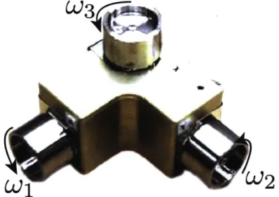
2-3 Enos' Universal Joint Cat.[15 . . . . 48 2-4 Pseudo-wheels are an example of a bounded shape change attitude

control actuator[40]. . . . . 48

3-1 A parallel free kinematic chain. . . . . 51 3-2 A serial free kinematic chain. . . . . 53 3-3 The model systems. All mass-centers are assumed coincident but are

depicted exploded for clarity . . . .-. . . . . 56

4-1 A hypothetical gait defined on a two dimensional shape space. Note the directionality in time, indicated by arrows. The area A is enclosed. 67

4-2 A change of coordinates for the No-Twist Cat. . . . . 70 5-1 Components of the curvature r. for the C' frame affixed to the No-Twist

Cat, witha= 2, b=0.1, c= 1, andd=2 . . . . 80 5-2 Comparison of two different circular gaits for the No-Twist Cat

ori-ented using the C' frame with different starting/ending points. Inertia

parameters are a = 2, b = 0.1, c = 1, and d = 2. . . . . 82

5-3 Three candidate gaits for the Universal Join Cat. . . . . 87

5-4 Components of the curvature r. for both the C" and the B frame affixed

to the Universal Joint Cat, with a = b = c = d = 1. Candidate gaits

are overlaid on the surfaces:

43

is detailed in blue,

#1

is detailed in yellow, and 02 is detailed in green . . . . . 89 5-5 Comparison of the quality of the cBVI approximation for the B and C'

frames affixed to the Universal Joint Cat with a = b = c = d = 1. The applied gait is

#1.

. . . . 90

(15)

5-6 The reconstructed result of the

#2

"figure-eight" candidate gait ap-plied to the C' frame affixed to the Universal Joint Cat demonstrates reorientation about the axis c'! However the accuracy of the cBVI approximation is clearly lacking. . . . . 90 5-7 Reconstructed trajectories of the orienting frame unit vectors for each

of the candidate gaits, through five gait cycles. The gaits

#5

are num-bered such that the numbers in the figure correspond both to gaits and to unit vector directions. . . . . ... . . . . 91 7-1 Catstronaut II. . . . . 105

(16)

(17)

Chapter 1 Introduction

Imagine you are floating in space, with nothing to push off of-and no rockets or thrusters at your disposal. (This is a somewhat scary hypothetical situation.) How would you move around? At least as regards translational motion, you are, sadly, out of luck, thanks to Newton's third law; no matter how much you flail, your center of mass is guaranteed to remain in exactly the same position for all time, given your aforementioned constraints. But you could change the direction you are facing, also known as your orientation or your attitude. This might be important if you want to signal to your fellow astronauts, or point your solar panels or solar sails towards a star.

We will address this orientation control problem herein, with particular interest in developing theory relevant to the design of attitude control actuators for very small satellites. This will lead to a demonstration of the storage of nonzero time-averaged angular momentum in a vibrating mechanical system, harnessing the finite stiffness of the structure to achieve useful control authority-an example of compliant robotics. More than a century ago, George Stokes and James Clerk Maxwell evidently also took an interest in compliant robotics:

He was much interested, as also was Prof. Clerk Maxwell about the same time, in cat-turning, a word invented to describe the way in which a cat manages to fall upon her feet if you hold her by the four feet and drop

(18)

her, back downwards, close to the floor.

[54]

The attempts of photographic and scientific pioneer Etienne-Jules Marey, a fasci-nating figure in his own right, to explain the phenomenon were chronicled in Nature in 1894:

M. Marey thinks that it is the inertia of its own mass that the cat uses to right itself. The torsion couple which produces the action of the muscles of the vertebra acts at first on the forelegs, which have a very small motion of inertia on account of the front feet being foreshortened and pressed against the neck. The hind legs, however, being stretched out and almost perpendicular to the axis of the body, possesses a moment of inertia which opposes motion in the opposite direction to that which the torsion couple tends to produce. In the second phase of the action, the attitude of the feet is reversed, and it is the inertia of the forepart that furnishes a fulcrum for the rotation of the rear.

[14]

Though his dynamical approach was controversial at the time,I with Marey's beautiful photographs (See Figure 1-1) inciting impassioned debate at the October

29, 1894 meeting of the Acad6mie des Sciences in Paris[13], the photographer was on

the right track! It is indeed an inertial phenomenon that leads to cat-turning, and the physics necessary to describe the phenomenon are directly relevant to the attitude control problem that this thesis seeks to investigate.

1.0.1 Motivation

Theoretical understanding of the control of an object's orientation is necessary in fields ranging from robotics to satellite design. We consider strategies for the reorientation, via cyclic shape changes, of a free deformable body in 3-space, or SE(3), acted on by no external forces or constraints except conservation of angular momentum.

As I see it, there are three main areas of application of these ideas:

'More scientists subscribed to the belief that the cat was using air resistance or pushing off of its handler.

(19)

Figure 1-1: Marey's falling cat chronophotographs.[14]

Fir. t.-Side view of a falling cat. (The series runs fr m right ko left.)

(20)

" MEMS-type (chip-printable) attitude control hardware that relies neither on

external interaction nor continuously-rotating mechanisms

* Attitude control of soft robots in space, underwater, and in other challenging environments

" Design of space structures where attitude control is directly integrated as

pre-existing hardware, to minimize necessary mass

We specifically consider the case where the conserved angular momentum of the deformable body is always zero; in practice, this would be the case for certain satel-lites and free-floating space robots. Systems of this type have been described in the literature as drift-free[32] and purely mechanical[47] (in fact, purely mechanical im-plies drift-free), meaning that they possess no momentum and that orientation is only a function of the time-history of internal shape.

For brevity, to pay homage to past work in the field, and to celebrate the real inspiration of this work, we refer to this dynamics and control problem simply as the

Cat's Problem. Somewhat confusingly, at least taxonomically, there is a subset of the

Cat's Problem that we will also give some time to: the Snake's Problem., which is really just the Cat's Problem but constrained to the plane (SE(2)).

Because of the purely mechanical nature of the system, the Cat's Problem is equivalent to formulating a control problem on a Lie group (a mathematical

ob-Kinematic Snake Floating Snake Differential-Drive Car

a,

a2 Center of mass a2 '0

b' (X, )

-a, a2

Passive wheels on links Net linear and angular momentum Driven wheels cannot cannot slip laterally of links cannot change slip or slide

Figure 1-2: Three textbook nonholonomic systems, borrowed with great thanks from Hatton and Choset[21].

(21)

ject describing the Cat's position and orientation), where the system's Lagrangian is invariant under the group action[48]-intuitively, the Cat dynamics are always the same, no matter the position or orientation of the Cat. There exist mathematical analogies to other canonical robotics models with nonholonomic constraints, chief among them the three-link planar snake and the differential drive vehicle. However, the Cat's Problem differs importantly in that the "nonholonomic constraint" (conser-vation of linear and angular momentum) falls out of the dynamics, so to speak, and is not externally imposed on the system (as is a rolling constraint, for example, which is the textbook nonholonomic constraint). This has the interesting consequence of ensuring the fully kinematic[47] nature of the angular-momentum-conserving system with zero momentum.

1.1 Conventional control strategies

Wi

Figure 1-3: Three orthogonally-mounted reaction wheels.

Spacecraft attitude control is provided by two possible means: shape change or interaction with the external environment. Thrusters that eject exhaust mass or ions are examples of attitude control methods that interact with the external environment (in that they transfer mass from the spacecraft to its environs), as is a magnetorquer, which relies on interaction with an external magnetic field to apply control torques

(22)

to the spacecraft, or an electrodynamic tether, which relies on interaction with an external ionic field. Thrusters are infeasible to build on very tiny scales, while electro-dynamic tethers have indeed been proposed for use on chip-based satellites[55]. We are interested in considering a theoretical basis for attitude control, implementable on very tiny scales, that does not rely on external interaction; therefore, we must rely on shape change.

A standard means of attitude control via shape change is the use of reaction wheels

or momentum wheels[53]. A reaction wheel is predicated on continuous rotation: by exerting a torque on an attached flywheel, a spacecraft feels an equal-and-opposite torque applied to itself. By mounting several reaction wheels, as in Figure 1-3, full control of spacecraft orientation is achieved.

However, continuously-rotating mechanisms are subject to relatively rapid wear, often require some sort of biasing to counteract stiction, and are challenging to con-struct and maintain on the microscale. Therefore, we are interested in systems that do not exhibit continuous rotation, but rather have bounded control inputs or shape degrees of freedom. This boundedness might be due to design constraints-it's hard to make a soft robot with continuously rotating parts, for example, or to make MEMS chips with rotating parts-or for other reasons (such as making a satellite with fully integrated attitude control hardware to save mass).

1.2 Nonholonomic systems

This is a difficult subject area! We give a very, very brief overview here; interested readers are strongly encouraged to consult the references.

We consider the configuration q of a dynamical system evolving on some configu-ration manifold

Q

(we can write q E

Q),

subject to some constraints, generically of the form f(q, q) = 0. Constraints of the form f(q) = 0 are termed holonomic and

only serve to reduce the effective dimension of the configuration space; i. e. we could use the constraint to define a constant submanifold of Q on which the dynamics are constrained to evolve. In this sense, holonomic constraints preclude controllability:

(23)

they prevent our system from ever touching certain parts of its configuration space

Q.

Figure 1-4: An illustration of (a) nonholonomic versus (b) holonomic constraints.

revolute joint

(a) (b)

Constraints of the form f(q, 4) = 0 are termed nonholonomic. A subset of

non-holonomic constraints are Pfaffian constraints[38], which are of the form w(q)q = 0. Importantly, nonholonomic constraints do not reduce the effective dimensionality of the configuration space; rather, they define what is termed a distribution, or a re-striction on the tangent bundle TQ of the configuration space. The tangent bundle contains all the possible directions the system could move in at every configuration; it is defined as a unique vector space, i. e. set of directions, at each point q on the configuration manifold. Intuitively, nonholonomic constraints define restrictions on the allowable directions the system can move in at a given configuration q. Because nonholonomic constraints do not reduce the dimension of the configuration space, they inherently allow a higher degree of controllabilty than holonomic constraints.

One might then attempt constructing equations of motion using a Lagrangian for-mulation or Hamiltonian forfor-mulation. Entire books have been written on the subject; the reader is referred to Bloch[5] for a very comprehensive overview of nonholonomic

(24)

mechanics.

Symmetry and reduction

Now, imagine that we have a system subject to nonholonomic constraints such that the configuration splits naturally into two parts q = (g, r), where g is an element of the orientation space G and r an element of the shape space M, such that

Q

= G x M is a product space; we have some map 7r that takes an element q

E

Q

and returns the corresponding orientation g

E

G. The group G is special: it is chosen exactly because the nonholonomic constraints are independent of its action, such that they depend only on the body velocity and not the world velocity

4

and thus can be written

f(

, r, r) = 0. This assigns the system the overall structure of a trivial fiber bundle,2

where we might term G the fiber space and M the base space. Intuitively, the shape

r parameterizes the "shape" of the system.

G =

SE(3)

-02 _O

xx

y 01

R.

- ( 1 -9 2)b1

+(9

-0 2)b3

Figure 1-5: An illustration of the relevant groups and velocities for the differential-drive vehicle. Note that due to the nonholonomic constraints on the wheels, the vehicle can only move forward in the b1 direction, or turn about the axis b3.

These are somewhat confusing and abstract ideas, especially if the reader is not group-theoretically inclined (please see Hatton and Choset's excellent coursebook[20] for an accessible introduction to this brand of mathematics), but some clarity might be

2

(25)

gleaned by considering the example case of locomotion, where g is taken to be the po-sition and orientation of a locomoting mechanical system, such as a differential-drive vehicle. In this case, it is clear that the nonholonomic constraints (the no-slip con-dition applied to each vehicle wheel) are independent of position and orientation-in short, the vehicle should "drive" the same no matter what its position and orientation are.

In the symmetrical nonholonomic case, it is possible to formulate the equations of motions of the shape r without reference to g (one can formulate the reduced

Lagrangian l( , r, r) and proceed from there); this process is called ronholonomic reduction[61. Conversely, it is also true that the shape trajectory r(t) uniquely

deter-mines the group trajectory g(t)-we speak, rather poetically, of lifting from the base to the fiber-which is a very useful property when considering the control theory of nonholonomic systems; this process is called nonholonomic reconstruction. A rigorous overview is given in

[33J.

Lie groups and algebra

Given the aforementioned mathematics, the group G also inherits the structure of a

Lie group. Every Lie group also has a corresponding Lie algebra, which is defined

as the tangent space at the identity element of the Lie group. For more in-depth discussion, the reader is referred to several references: Again, Hatton and Choset[20] provide an accessible introduction; while Boothby[7] or Abraham[l] provide a more rigorous treatment of the fundamentals.

Drift

The term drift refers to "dynamics in the absence of controls";3 intuitively, imagine the ability of the mechanical system to "coast", or to acquire momentum p (generalized

nonholonomic momentum in the terminology of Bloch[5l). We are concerned with drift free systems, in that they have no nontrivial dynamics without control inputs

(some kind of activation of the shape r)-as an example, remember the

differential-3

(26)

drive vehicle and note that it will only move if the wheels (controls inputs) are turning. This feature implies that drift-free systems have the same number of nonholonomic constraints as dimensions of the fiber space G.

Figure 1-6: Ostrowski[42] provides the example of the snakeboard: a symmetric non-holonomic system with nonzero drift.

back wheels

0 front wheels

Drift-free also implies that the relationship between the shape r and the orientation g is determined only by the nonholonomic constraints, and not by the evolution of a dynamical equation; therefore, it is independent of time parameterization.

Mechanical vs. dynamical nonholonomic constraints

In the literature, there is the further distinction between purely mechanical[47] and

principalfly] kinematic[41] systems. These systems are characterized by the specific

type of nonholonomic constraint that defines their dynamics: mechanical or dynamical

([5]

p.18 5). Mechanical constraints are defined as nonholonomic constraints that are

externally-imposed on the system, such as rolling constraints. Dynamical constraints are those that "fall out of" a momentum conservation law; importantly, they are only invariant under the group action if p = 0.

Principally kinematic systems cannot ever have p 4 0 (strictly speaking, p is not even defined) and arise when the number of mechanical nonholonomic constraints is exactly equal to the dimension of the group space; examples include the differential drive vehicle and the three-link kinematic snake[18]. It is important to note that the principally kinematic nature of a system with mechanical nonholonomic constraints

(27)

is contingent on design alone; as in, the designer must specifically choose to have the same number of mechanical nonholonomic constraints as group dimensions if he wants to create a principally kinematic system (for example, the kinematic snake must have exactly three links in order to be a fully kinematic system).

Purely mechanical systems differ in that p exists but the dynamics are such that

0 and thus p stays constant for all time; these are simply systems that conserve

momentum. If we pick a purely mechanical system and "start" it such that p(O) =

0 -+ p(t) = 0, it will evolve exactly as a principally kinematic system: Per Noether's

Theorem (CITE something? Goldstein), the number of conserved quantities (the momenta p) is guaranteed to be exactly the dimension of the Lie group G, since the system is symmetric with respect to G. In general, the geometric phase and dynamic

phase[5] decouple for purely mechanical systems. Examples of purely mechanical

systems include the floating snake, planar snake robot[18], and of course the falling cat.

1.2.1 Reconstruction

The analysis of nonholonomic systems is concerned with reduction, as aforementioned, and reconstruction[6]. The reconstruction process aims to reconstruct the fiber tra-jectory g(t) given the base tratra-jectory r(t) determined via reduction. We will be considering systems where the reduction process is simple: either the shape r is fully actuated and no nontrivial reduction is necessary since r(t) can be specified directly, or r is underactuated but since p = 0 the reduced dynamics are straightforward to

derive.

The reconstruction equation[19] applies generally to all nonholonomic systems with symmetry:

We sep) = -A(r)+p a ) b (1f1

(28)

= (TeL)-1 = TgLg-1i (1.2)

Where the operator TeLg represents a left lifted action (see Hatton and Choset's coursebook[20 for an accessible explanation). Suffice to say here that, in the case of matrix Lie groups, TeLg = g and thus = g-'4. In a locomotion context, this is equivalent to an object's velocity vector expressed in its body-fixed frame.

Therefore, for principally kinematic systems with matrix Lie groups only:

y = -gA(r)r (1.3)

The matrix A(r) is referred to as the local connection, and it encodes the rela-tionship between the shape r and the orientation g.

Equation 1.3 is ubiquitous in the literature. It is the underlying equation that al-most all nonholonomic control systems are based off of; we might consider the control input to be u A . Our task, now, as control system designer, is to put our particular systems of interest into the appropriate mathematical form, and then to determine the control input trajectories u(t) that yield desirable orientation trajectories g(t).

In general, it is difficult to invert Equation 1.3 (i.e. to solve for the r(t) that produces a specific g(t), instead of vice versa), and so a variety of mathematical tools have been developed to aid in the design process. The concept of "desirability" also must be quantitatively defined, and, indeed, it is in the field of optimal control theory, which seeks to identify the "best" (perhaps the minimum energy, for example) trajectories that achieve a desired result (often, a desired holonomy, which will be defined below).

Geometric phase

Given a system with nonholonomic constraints and symmetry, it is possible to gener-ate a base trajectory r(t) that is cyclic-such that r(t+T) = r(t)-but that results in

a nonzero change in orientation-such that g(t + -r) # g(t). We will later define these trajectories more formally as gaits. For a principally kinematic system, this fact can

(29)

Figure 1-7: Bloch[5] provides a useful visualization of lifting from the base space to the fiber space. This also visualizes the geometric phase or holonomy associated with a closed curve in the base space.

vertical direction horizontal directions

bundle

geometric phase

bundle projection

base space

be verified by directly integrating the reconstruction equation.

As a very simple example borrowed from Bloch[5], consider the idea of parallel

transport on the sphere: a vector traverses a closed loop on the surface of a sphere,

always pointing in the same local direction; by the time it reaches its starting point, its pointing angle has changed. The change in pointing angle is proportional to the area enclosed by the closed loop.

In the literature, this change in orientation h - g(t+T) -g(t) due to a closed curve in the base space has been termed the geometric phase[29][25][30], or holonomy[5] associated with the base curve (in quantum physics, it is also called the Berry phase). Correspondingly, any change in orientation due to drift (nonzero momentem p), if it exists, is termed dynamic phase[5]. These concepts solidify the connection between holonomy and path dependence.

1.2.2 Rectification

In the context of this work, we define mechanical rectification, using terms borrowed from electrical engineering, as some kind of DC (i.e. secular, non-zero time-average) motion resulting from AC (i.e. periodic, cyclic) motion. This framework is in large

(30)

Figure 1-8: Bloch[5 provides another useful visualization of geometric phase in the example of parallel transport on the sphere.

area =A finish

start

part due to Brockett[9]. One can imagine the internal combustion engine as perhaps the most ubiquitous example of mechanical rectification.

Connection to the Lie bracket

Mechanical rectification is related to the Lie bracket: the Lie bracket is, in some sense, the mathematical encoding of a system's ability to exhibit mechanical rectification. Therefore, it is also related to path dependence, which is fundamentally related to

[non]holonomy.

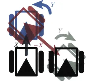
An intuitive physical explanation of the Lie bracket is parallel parking the text-book differential-drive vehicle from earlier: The differential-drive vehicle can only steer, or move ahead in the direction defined by its steering angle; it cannot move sideways, due to the nonholonomic rolling constraint on the wheels. Thus, it can directly access only a subset of its tangent bundle-it is not free to move in all pos-sible directions at any given time (recall that this is called a distribution). However, through a parallel-parking-sort-of-maneuver (gait; sequence of motions), which

(31)

in-Figure 1-9: Parallel parking a differential-drive vehicle is a simple explanation of the Lie bracket.

Y

- Y

X -X

volves a combination of steering and driving, the car can indeed move sideways, even if we shrink the steer/drive-wiggle to a differentially small size-this wiggle is in fact a physical explanation of the Lie bracket of this particular system.

Intuitively, the Lie bracket [X, Y] involves flowing the system differentially along a vector field X (let's call this moving forward a tiny bit), then along another vector field

Y (this is turning just a little counterclockwise), then along -X (moving backward

a tiny bit), then along -Y (turning just a little clockwise). We can imagine that as these motions in sequence get very small, the car ends up moving slightly sideways, directly to its right. Thus, the car is able to move in the b2 direction, a direction that

is not part of the subspace of the tangent space that the nonholonomic constraint distribution dictates (remember that it stipulates that a car may only move forward or steer)! Therefore the distribution is not closed under the Lie bracket-i. e. the Lie bracket yields a vector that is not a member of the space spanned by X and Y. And we see, now, that the Lie bracket is a kind of differential operator, and that the Lie bracket of two vector fields is also a vector field.

If we define the vector fields X and Y using arbitrary functions-X =

f(q)

and

Y = g(q) for q E

Q-then

the Lie bracket is[38]:

[fg](q) = 0f(q) - g(q) (1.4)

(32)

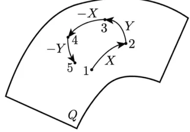
Figure 1-10: The Lie bracket visualized as a differential sequence of flows along two vector fields. Note the noncommutativity: the starting point is not the ending point.

-X

3 Y

_y

2

5

iX

If we define the vector fields X and Y using matrices-X = Aq, and Y =

Bq-then the Lie bracket s is the matrix commutator:

[A,B] = BA - AB (1.5)

This demonstrates that the Lie bracket is fundamentally an expression of the

noncommutativity of the underlying vector fields. Noncommutativity is connected to

the idea of path dependence (or ordering, if we are still thinking in terms of matrices), a concept that we have seen before in the context of holonomy!

To be technical, the Lie bracket is an operator that is applied to elements of the

Lie algebra g corresponding to the Lie group G. In many contexts, the Lie algebra can

be thought of as a generalization of velocity. For example, if our Lie group is SO(3), which is the space of all 3D rotations, then the corresponding Lie algebra is so(3), which is the space of all 3D angular velocities. Recall that, in general, the Lie algebra is identified with the tangent space at the identity element of the Lie group (meaning that, more technically, so(3) is the space of all body-fixed angular velocities).

It can be proven that the Lie bracket of two angular velocity vectors x, y E 5o(3) is the standard vector cross-product:

[x,

y] = x x y.

(33)

com-prised of periodic (AC) motions (in our differential-drive vehicle example, a combina-tion of moving forwards/backwards and steering left/right) that results in a net (DC) motion (in our example, moving to the right).

[Non]involutivity

A distribution is called involutive if it is closed under the Lie bracket. Via the

Frobenius theorem, we know that a distribution is integrable iff it is involutive[38]. therefore, a nonholonomic constraint is by definition not integrable (this actually follows from the fact that nonholonomic constraints do not reduce the dimensionality of the system configuration).

Any system with nonholonomic constraint(s) has some kind of "parallel-parking ability"-which means that one can use a clever periodic sequence of motions (gaits) to produce meaningful motion that would otherwise be unavailable. One might imagine that this property is useful in a robotics context.

Further, there is a deep relationship between underactuated and nonholonomic systems-nonholonomic systems are necessarily underactuated: We don't control g directly, but indirectly through the manipulation of r. This segues into the next subsection.

1.2.3 Controllability

Controllability of nonholonomic systems seeks to answer the following: by manipu-lating the available control inputs (usually, the shape variables r, assuming that the shape space is fully actuated), is it possible to drive the system to any point in the full configuration space (both the shape space and the orientation space)?

Rigorous treatment of the accessibility and controllability4 of nonholonomic sys-tems is given by Kelly and Murray[25]. In particular, they demonstrate that if the underlying (fiber) Lie group is abelian (i. e. the Lie group is commutative: the Lie bracket is identically zero), the net holonomy (i.e. the net result of the lifted

tra-4_{These are subtly different concepts... technically, accessibility and controllability only differ for}

(34)

jectory through the fiber space) associated with a closed trajectory r(t) in the base space (the shape space) is directly proportional to an integral of some vector field (re-lated to the curvature[1] of the local connection) over the area enclosed by r(t). This result is termed the area rule and is also discussed by Leonard[31] [32]. An example of a system in which the underlying Lie group is abelian is in fact the floating "space snake" proposed by Hatton and Choset[21], where G = SO(2) (See Figure 1-2).

This result emphasizes the fact that "non-abelian" and "nonholonomic" are not synonymous! Just because the underlying Lie group is commutative, the system can still exhibit path dependence (holonomy)-the entire configuration group

Q

can still be noncommutative.

The central theorem of noholonomic controllability is due to Chow; sometimes

called Chow's Theorem or the Chow-Rashevsky Theorem.5 Chow's theorem is

es-sentially a statement about the "directions" that a system can move in at a given configuration: if at every configuration q E

Q

these directions span the entire tangent space, then the system is fully controllable. Some of these directions may have to be generated with Lie brackets, or even Lie brackets of Lie brackets (these would be termed higher-order brackets). This process is often referred to as iterated Lie

bracketing[44].

For non-abelian Lie groups-including SO(3) which is the focus of this thesis, and SE(2), which is one of the most common spaces for simple locomoting robots, such as the differential-drive vehicle, to live in-the area rule does not apply. However, Hatton and Choset[21], building upon the work of Radford and Burdick[44], have developed an approximate area rule, which they have termed the corrected body velocity integral, or cBVI.

Feedback control

Reyhanoglu and McClamroch[46] conclude that a certain class of nonholonomic sys-tems (a subset of the Snake's Problem, actually) cannot be feedback stabilized about

5

The earliest reference I can find in the literature is to Rashevsky's "Any two points of a totally nonholonomic space may be connected by an admissible line" which is in Russian and from 1938.

(35)

arbitrary equilibria using a smooth (Cl) feedback control law. This makes some intu-itive sense-a nonholonomic system can be fully controlled but has to do a "parallel-parking wiggle" in order to move in certain directions; this wiggle cannot be captured

by standard feedback control laws. As a consequence, the development of robust

feed-back control laws for nonholonomic systems is complicated; fundamentally, a degree of open-loop control is necessary. This is embodied in the control strategy proposed

by Leonard[32], which is comprised of open-loop control interspersed with periodic

closed-loop "checkups".

1.2.4 Steering

Determining theoretical controllability is not the same thing as ascertaining the actual control input trajectories that would provide useful motions, which we would term

open-loop motion planning or steering.

Brockett has shown that, for systems that require only one "level" of Lie bracketing, sinusoidal inputs are optimal[8l, in the sense that they minimize energy.

Murray and Sastry[39] expand upon Brockett's result to demonstrate motion plan-ning for systems that require higher order Lie brackets, showing that sinusoidal inputs at integrally-related frequencies can be used to steer the system.

1.3 Attitude control via shape change

A mechanical system that conserves net angular and linear momentum, as

aforemen-tioned, has the mathematical structure of a symmetrical nonholonomic system with symmetry. The underlying Lie group is G = SO(3) C SE(3), which is the space of all 3D rotations.' The corresponding Lie algebra is so(3), which is the space of all

3D angular velocities.

Because of this mathematical structure, we expect these sorts of mechanical sys-tems to have a "parallel parking ability" which can be used to control their orientation

6_{We do not have to concern ourselves with linear translations because conservation of linear}

momentum is always an integrable constraint, meaning that it reduces the dimensionality of the underlying Lie group from SE(3) to SO(3).

(36)

g E G.

1.3.1 Group structure

This representation (Equation 1.3) makes it clear that, for angular-momentum-conserving systems, the columns of the local connection A(r) are themselves elements of the "an-gular velocity space" so (3). The Lie bracket is the vector cross product (one can note that, for groups that are matrix spaces, the Lie bracket is equal to the matrix com-mutator, and the matrix commutator of two skew-symmetric matrices is equal to the cross product of the corresponding vectors). This sets up a natural isomorphism be-tween so(3) and R3-meaning that the skew-symmetric-matrix-representation with matrix commutator Lie bracket is equivalent (isomorphic) to the representation with

angular velocity vectors Q E R3 with vector cross product Lie bracket.

For these systems, the reconstruction equation (Equation 1.3) is equivalent to transforming the angular velocity vector from the affixed frame C to the inertial

frame I. If we represent g with rotation matrices, Equation 1.3 becomes:

wIcr~ (1.6)

dt

1.3.2 Prior work

The fields of geometric control theory and nohononomic mechanics are rich and well-developed. Marsden, Montgomery, and Ratiu{33] provide a comprehensive treatment of classical mechanical systems with symmetry; Bloch[5] provides a good overview of nonholonomic mechanics; Bullo and Lewis[10] provide a nice overview of the control theoretic aspect. We do not attempt to fully summarize the entire subject in this section, but rather to summarize the connection to shape change attitude control.

There exists a substantial body of literature dealing specifically with attitude con-trol via shape change of a deformable body. The field was debatably initiated (though references to the Cat's Problem existed in the literature before this, with the earliest theoretical treatment given by Rademaker and ter Braak[43]) by NASA, providing

(37)

Figure 1-11: Rademaker and ter Braak[43] did not have as good of a photographer as Marey.

Abb. 1.

Freier Fall in Rtickenlage.

I. Norinale Katze mit verschlossenen Augen. Das Tier dreht sich in der Luft.

(38)

funding to researchers in the late 1960s (exemplified by Kane and Scher[22][23]).

NASA was interested in obvious practical application to spaceflight. The work of

Kane was then picked up in the early 1990s by physicists like Montgomery[36][37], Enos[15], and Shapere[50] who realized the connection between the Cat's Problem and what physicists would call gauge theory (i.e. studying dynamical systems with useful symmetries, often in the context of particle physics). Shapere, with Wilczek who would go on to win a Nobel Prize in physics, had realized this gauge theoretic con-nection first for the low Reynolds number locomotion of deformable bodies[51]-in certain scenarios, the Stokes equations can be reduced to a set of linear nonholo-nomic constraints-and went on to write his PhD thesis on the Gauge Mechanics of

Deformable Bodies[49].

This work united the Cat's Problem with ideas in geometric mechanics and differ-ential geometry (which had been applied to other gauge theoretic problems; par-ticularly ideas about Lie algebras and controllability, developed in large part by Brockett[8j) and opened the field up to engineers-see the work of Krishnaprasad on geometric phase and the Cat's Problem[29][30], McClamroch on the shape control of spacecraft[34][52] 7 and Chen[11][12], who considered the Cat's Problem as applied to satellites.

Leonard[31] [32] proposes the model system of a spacecraft with a point-mass oscil-lator (which provides the ability to change shape) as an example of motion planning and control on Lie groups.

Ananthasuresh and Koh published some work in the early 2000s on what they term "pseudo-wheels", which are in essence shape change attitude control actuators that are a specific instantiation of the Cat's Problem[26] [27] [40].

7

McClamroch and his students built the first real experiments dealing with shape change attitude control[4}, as far as I know

(39)

Chapter 2 Background

In this chapter, we formalize some notions about angular-momentum-conserving sys-tems that have been touched upon. Please refer to Appendix A for an overview of the notational formalisms employed in this thesis. Three dimensional kinematics can get very complicated, and it is useful to have a standardized notation for vectors, rotations, and other transformations.

2.1 Free deformable bodies

Free deformable bodies, as defined in this body of work, are simply dynamical systems comprised of elements that are constrained to always behave a certain way in relation to each other, that exhibit a certain important symmetry, and that conserve angular momentum.

2.1.1 Free systems

This important symmetry is translational and rotational invariance; in mathematical terms, free systems are invariant under the action of the group SE(3), which is the group of all non-mirroring (direct isometries, orientation preserving) 3D translations and rotations. By SE(3) invariance, we just mean that the dynamics of the free system do not care what the position or orientation in 3-space of the system is. A

(40)

free system also conserves angular momentum; this means that the free system does not interact at all (does not apply any forces or torques to) with anything else in 3-space--it is free in this sense.

2.1.2 Deformable bodies

Deformable is somewhat trickier to quantitatively define. It is not hard to intuitively

define: a deformable body can change its shape, like a folding chair, or a water balloon, or a pair of scissors, or even a house cat. Some deformable bodies can change shape internally, using only internal forces and torques (e.g. the house cat), but some deformable bodies can only change shape passively, due either to applied external forces (particular solutions; e.g. unfolding the folding chair) or to dynamical effects (homogeneous solutions; e.g. the water balloon vibrates if you poke it). It is clear that the notion of deformability is intrinsically linked to the ability of a system to qualitatively change shape.

So perhaps we can define deformable bodies by first defining their dual: rigid bodies. A rigid body can be thought of as a system of infinitesimal particles that are related by a very specific constraint: that the relative positions between all the infinitesimal particles are always the same; intuitively, the shape of a rigid body cannot change. This allows us to assign lumped parameters to rigid bodies such as mass and moment of inertia. Similarly, we might consider linear springs, dashpots,

etc. as lumped parameter constraints.

Deformable bodies account for all the other possible mass-conserving systems of particles. The slightly vague stipulation that deformable bodies must still be "whole" or "cohesive" seems to me to be a kind of heuristic based on the types of deformable bodies that we tend to experience: Is a system of particles that interact only via electric charge a deformable body? Maybe not in the practical sense, but maybe yes in the mathematical sense. It also might help to somewhat-arbitrarily impose some sense of mass conservation: deformable bodies cannot lose mass. In this sense, we could consider a half-full water-bottle to be a deformable system (if capped), but a control-volume section of a pipe conveying water not to be. Similarly, if we

(41)

Figure 2-1: Three examples of deformable bodies: (a) a rubber band (modeled as a collection of infinitesimal point masses); (b) a pair of scissors; (c) a free Euler-Bernoulli beam with sprung masses on the ends and a rigid body in the middle.

P-

W

P lPi

P~(t)

(a) (b) (c)

take a rocket ship to be only the rocket-with-onboard-fuel, it is not a deformable body as defined, as it is constantly ejecting exhaust mass, but we might consider the rocket-fuel-exhaust system to be a deformable body, since mass conservation is always retained.

Obviously, the particular nature of a deformable body is very much determined

by the nature of the relationship (or constraint) between constituent infinitesimal

particles. Perhaps the archetypal deformable body is a rubber band. If we model a rubber band using linear elasticity theory, we can think of it as a collection of infinitesimal particles joined by linear springs. Similarly, an Euler-Bernoulli beam can be thought of as a series of infinitesimal particles joined by torsional springs; a fluid can be thought of as a collection of infinitesimal particles that transmit normal and shear stresses to neighboring particles. These are all examples of continuums, in that one typically analyzes the behavior not of the individual infinitesimal particles that comprise the system but of the bulk.

But a deformable body need not be a continuum body in the strict sense: consider a pair of scissors, or two rigid rods joined by a revolute joint. This is obviously not a continuum in the sense described above, but is still a deformable body.

(42)

Shape of deformable bodies

Deformable bodies are characterized by their shape, which intuitively prescribes the relative position between all the component particles P that comprise the deformable body (we see that the shape of a rigid body is always constant, since for a rigid body this set of relative positions is constrained to always be constant). In general, we represent the shape with a vector r of variables that parameterizes the shape; in the example of the scissors, we could say r - 0. Also in general, the shape representation r is not unique.

We say that a point

Q

is fixed to the body if its position rQ/P, relative to all points

Pi in the body is a function of the shape representation r only.

The distinction between the shape itself and the corresponding shape

represen-tation is subtle, both semantically and mathematically. It is something like the distinction between a vector, as a more abstract object that lives somewhere on a manifold and has unambiguous direction and magnitude, and the set of coordinates that parameterize the same vector. Often, we are able to make statements and do some calculations without parameterizing, but, at least in engineering, we need to plug in values eventually and to do so we need to parameterize. The subset of math-ematics that is best situated to resolve these sorts of ambiguities and confusions is group theory, which explains the prevalence of group theoretic notation and rhetoric in the relevant literature.

In the example case of scissors, we need just one parameter to define the shape: the opening angle 6 of the scissors. In the case of the rubber band, the shape is defined by the position rP/G of each infinitesimal particle P, relative to some reference point

Q

fixed to the band, and so we need an infinite number of variables to define the shape: Continuum bodies are infinite dimensional. In general, the dynamics of n-dimensional deformable bodies are determined by 2nth order ordinary differential equations, while the dynamics of continuum bodies are determined by partial differential equations (e.g. the Navier-Stokes equations for a fluid, or the Euler-Bernoulli equations for a beam).

(43)

One can also envision deformable bodies that are combinations of both continuum and rigid lumped-parameter elements: for example, consider an Euler-Bernoulli beam with a rigid body attached to the end via a linear spring. In this case, the system dynamics are determined by coupled ODEs and PDEs.

Position and orientation of deformable bodies

The global position of a deformable body can be defined by keeping track of the position rG/O of one infinitesimal point G fixed to the body; it sometimes makes sense to define the center of mass of the deformable body to be this reference point, just as is the case with a rigid body.

But while it is straightforward to define one orientation for a rigid body R-represented by the rotation transformation 'RE necessary to rotate the body from a reference orientation (which is identified with the fixed inertial frame X) to the real orientation as the reference point stays fixed-it is nontrivial to define the same for a deformable body, for the simple reason that the relative position of each constituent element of the deformable body changes as the shape changes. In a simple case-the scissors, again, for example-we might keep track of the orientation of just one of the rigid elements in the standard rigid-body way, and in this way define an orientation for the entire deformable body; but it is not immediately clear how we would define the orientation of a rubber band, which has no rigid elements that are "easy" to keep track of!

To try and tackle this issue quantitatively, we define the global orientation of the deformable body as the orientation of some reference frame C relative to the inertial frame 1. However, in order to do useful engineering mathematics, we also need to pick a suitable representation g for the orientation of C, much in the same way that we chose a representation for the shape r. This amounts to choosing a set of parameters g that defines the rotation transformation IRC. This could directly be a rotation matrix (g IRc)-or it could be some other set of parameters, such as a quaternion

-or set of Euler angles (-TRC(, 0, /) -+ g A [0, 0, 0]T) that defines the same rotation.

(44)

defined only by the position rp,/Q of points P on the body relative to a point Q fixed to the body in the aforementioned sense. Therefore, if we know the global position and orientation as well as the system shape r, the position of any point on the system can be determined. The simplest example of this sort of frame is the body-fixed frame

Ai of any component body in a deformable system comprised of multiple rigid bodies joined by kinematic constraints: IRC A IRAi. Another appropriate candidate for a C frame is any of the

A,

rotated or translated by an amount that is a function of the system shape: IRC A T(r) IRAi. We refer to C as the orienting frame.

2.1.3 Actuation and reduced dynamics

Because we are interested in control, we are interested in deformable bodies that are internally actuated: they have some means of altering their shape via internal forces or torques, termed control torques. We are also interested in investigating systems where useful changes in shape can be sustained or effected by dynamical effects, specifically stiffness.

Therefore, we consider the case where the shape space of the system is not fully actuated: i.e. where we do not directly actuate all the parameters in r, but instead let some evolve passively via dynamic constraints (e.g. springs and dashpots inside the joints). In this case, we refer to the shape space as underactuated. Note that the kinematic case and dynamic case are equivalent for fully actuated shape spaces, since one could always use the inverse system dynamics to calculate the joint torque trajectory necessary to create a desired joint trajectory.

2.1.4 Boundedness of the shape space

As alluded to before, we would like to consider the case where the shape space is

bounded. This corresponds to many real deformable bodies: no joint in the human

Attitude control via structural vibration : an application of compliant robotics

Attitude Control via Structural Vibration:

application of compliant robotics

Nathan S. Tyrell

@

...

Signature redacted...

redacted

Signature redacted

JUN 21 2017

LIBRARIES

Attitude Control via Structural Vibration: an application of

compliant robotics

by

Nathan S. Tyrell

Abstract

Acknowledgments

~:

Contents

List of Figures

43

#1

#1.

#2

#5

Chapter 1

Introduction

[54]

[14]

1.0.1

Motivation

1.1

Conventional control strategies

Wi

1.2

Nonholonomic systems

Q

Q),

Q.

revolute joint

Q

E

Q

E

4

f(

G =

SE(3)

xx

R.

+(9

[33J.

([5]

1.2.1

Reconstruction

1.2.2

Rectification

[non]holonomy.

f(q)

Q-then

-X

3

Y

_y

2

5

[x,

1.2.3

Controllability

Q

Q

1.2.4

Steering

1.3

Attitude control via shape change

1.3.1

Group structure

1.3.2

Prior work

Chapter 2