Asteroseismic Study of the Subgiant HD 82074

Asteroseismic Study of the Subgiant HD 82074

A__

INSTfl1JE-by

Victoria Ashley Villar

[j

5204

Submitted to the Department of Physics

LIBRARIES

in partial fulfillment of the requirements for the degree of

Bachelor of Science in Physics

at the

MASSACHUSETTS INSTITUTE OF TECHNOLOGY

June 2014

@

Massachusetts Institute of Technology 2014. All rights reserved.

Signature redacted

Author.

Department of Physics

Signature redacted

May

9,

2014

Certified by..

Certified by....

Signature

. .. .. . .... . .. .. . .... ... . .. .. .. ...

John A. Johnson

Harvard Department of Astronomy

redacted

Supervisor

Joshua N. Winn

Department of Physics

Thesis Supervisor

Signature redacted

Accepted

by...

Nergis Mavalvala

Senior Thesis Coordinator, Department of Physics

Asteroseismic and Interferometric Study of the Subgiant HD

82074

by

Victoria Ashley Villar

Submitted to the Department of Physics on May 9, 2014, in partial fulfillment of the

requirements for the degree of Bachelor of Science in Physics

Abstract

This thesis analyzes HD 82074, a solar-mass and low-metallicity subgiant star, using ground-based asteroseismology with the CHIRON spectrometer at the Cerro Tololo Inter-American Observatory (CTIO) and interferometry with the CHARA array on Mt. Wilson. The physical parameters of subgiant stars are of particular interest in the exoplanetary field due to their importance in understanding the relationships between planet occurrence rate and stellar properties such as age, metallicity and mass. Potential systematic uncertainties in the canonical stellar models make it especially important to independently determine the masses and radii of these stars. We determine HD 82074's radius using interferometry from CHARA, and we combine this result with measurements of the spacing and frequencies of the asteroseismic oscillations of HD 82074 to determine a stellar mass. We find that the star has a radius of 3.96 0.12 solar radii and a mass of 1.20 0.11 solar masses. While the radius is in excellent agreement with predictions from spectral analysis, the mass is 2.9-o- greater than the predicted mass. This suggests that errors of stellar models may be underestimated for low-metollicity or evolved stars. This study makes HD

82074 the third subgiant for which a physical radius is confirmed interferometrically

and one of ten asteroseismically studied subgiants. Thesis Supervisor: John A. Johnson

Title: Professor of Astronomy Thesis Supervisor: Joshua N. Winn Title: Associate Professor of Physics

Acknowledgments

Foremost, I would like to express my deepest gratitude to Professor John Johnson and Professor Joshua N. Winn, my research supervisors, for their guidance, patience, support and valuable critiques of this thesis. Being a member of Professor Johnson's research group for the past year has been an incredible learning experience, and I am grateful for the opportunity.

I would also like to thank my collaborators: Professor Debra Fischer, Tabetha Boyajian and Tim White for their advice and contributions to this work. My gratitude is also extended to the SMARTS observing team.

I thank my friends for keeping me grounded and Alex McCarthy for his selfless aid and encouragement.

Finally, I wish to thank my family for their continuous support throughout my entire academic career.

Contents

1 Introduction 17

2 Theoretical Background 25

2.1 Excitation and Restoration Processes ... 25

2.2 Spherical Harmonics . . . . 28

2.3 Asymptotic and Scaling Relations . . . . 28

2.4 Theoretical Spectra . . . . 33

2.5 Constraints on Radius from Interferometric Measurements . . . . 37

3 CHIRON Radial Velocity Measurements 41 3.1 Target Selection ... 41

3.2 Observational Strategy ... 42

3.3 CHIRON Observations ... 44

4 CHARA Interferometric Observations and Results 49 4.1 CLASSIC Observations . . . . 49 5 Analysis ₅₃ 5.1 Significance Spectra. ... 53 5.2 Determining vm .... ... ... .... 56 5.3 Determining Av ... . .. ... 58 6 Results 65

List of Figures

1-1 Confirmed exoplanets from The Extrasolar Planets Encyclopedia. Five

methods of exoplanet detections are shown: radial velocity measure-ments which are described in the text (blue stars); Transiting planets which uses the dip in stellar light as an exoplanet passes in the line of sight (red circles); Microlensing which searches for abnormalities in typical microlensing events as two stars overlap in our line of sight (black triangles); Timing variations which arise from pulsar signal vari-ations or varivari-ations within another exoplanet's orbit. These methods

cover distinct ranges of parameter space for exoplanets. . . . . 18

1-2 HR diagram showing B-V color versus absolute V magnitude of host stars with planets found before May 2011. Hosts with M. > 1.5Meare

shown in filled circles, while hosts with M. < 1.5Meare shown in open

circles. The dotted-line box shows the parameter space of the sample

of evolved stars in Johnson et al. (2006) (0.5 < Mv < 3.5; 0.5 < B-V

< 1.0). The shaded region contains 28 hosts with M. > 1.5MDand 3

with M. < 1.5MO. The lines are evolutionary tracks of hosts of 1.2, 1.5

and 1.8Meranging in metallicity from -0.4 to 0.2. These tracks were derived from Yonsei-Yale isochrones. Figure taken from Lloyd (2011)

2-1 Propagation of acoustic and gravity waves in a Sun-like star. Panel (a) demonstrates how the p mode paths bend radially outwards with increasing depth, until reaching their various inner turning points" and undergoing total internal refraction. Panel (b) traces a g mode ray path which is trapped in the inner radiative layer of the star. The ray path

of the g modes depend heavily on the star's core conditions [22, 2].

Figure taken from Aerts et al. (1996). . . . . 27

2-2 Sample spherical harmonics, Y"(0,

#).

per-tubation while red reresents a negative perturbation. Image taken from

Ahern (2009) [3] . . . . 29

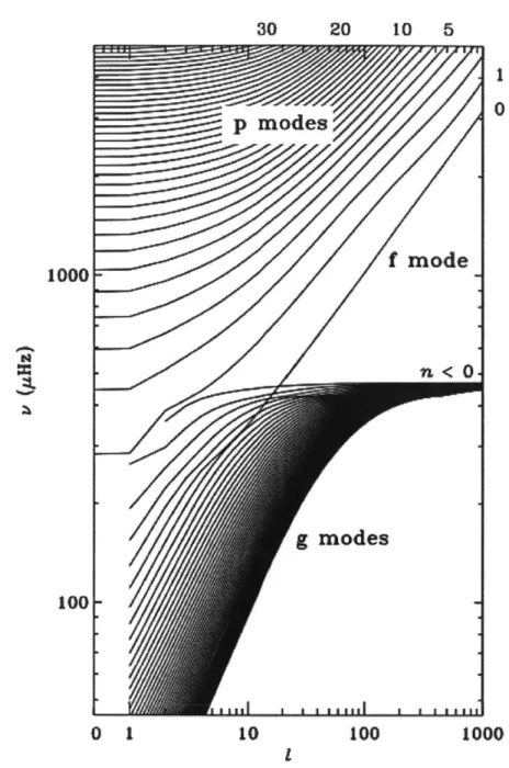
2-3 Frequency of modes versus their degree I for a Sun-like star. In the

upper right corner, a few corresponding overtones (n) are listed for reference. The overtones for the g modes are negative by convention. Solid lines, rather than discrete modes, are used for clarity. The figure illustrates that p modes increase in frequency with increasing overtone and degree, while g modes decrease with overtone but increase with degree. A single f mode is seen crossing the phase space of both g and

p modes. Figure from Aerts et al 2010 [19]. . . . . 30

2-4 Example of an asteroseismic "HR" diagram. Here, a function of effec-tive Temperature Tf is plotted against a function of Av and

metalli-ciy [Fe/H]. The colored tracks represent masses ranging from 1.3M0(in

magenta) to 1.6M0(blue) in steps of 0.1MG. The line types represent

different metallicities, shown in the legend. The tracks beging to over-lap in the shaded grey region. Figure taken from Lundkvist et al.

2-5 Spatial response functions integrated over a uniformly illuminated disk

for different mode degrees, with m=0. (Note that a change in m cor-responds to a change in the overall orientation of the harmonics. The effect of orientation is shown in Figure 2-6. The red model shows the response function in photometric data, while the blue model shows the expected response in RV measurements. The dotted lines account for

limb-darkening of the form W(O) = 1 - 0.75(1 - cos(9)) + 0.22(1

-cos2_{(0)) [54, 17]. A negative value of the spatial response function}

in-dicates that the overall response is less than the unperturbed reference. 35

2-6 Mode visibility as a function of stellar inclination angle. Modes vary

in I and m. Colors signify I values of 0 (blue), 1 (red), 2 (green) and

3 (black). Line styles represent m values of 0 (solid), 1 (dotted), 2

(dashed) and 3 (dot-dashed). [54] . . . . 36

2-7 Power spectrum of solar oscillations, obtained from radial velocity

mea-surements in light integrated over the full disk of the Sun. The data has a temporal baseline of approximately 15 years, revealing incredible details in the velocity spectrum. Panel (b) shows a zoomed-in version of panel (a) and highlights the standard asteroseismic observables, as well as the degree classification for a selection of the models. Figure

taken from Aerts et al. (2010) [2]. . . . . 39

2-8 Echelle diagram for observed solar frequencies obtained with the Bi-SON network. The frequencies are modulo Av = 135pHz (described

as "reduced" frequency) with v. = 830pHz. The degree of the modes

are indicated by the shapes. The deviation from the expected vertical-line model is evident for very low frequencies. Figure from Aerts et al.

(1996) [2]. . . . . 40

3-1 Sample of the Gaussian envelop of frequencies used to generate the

simulated stellar oscillations. Solar parameters were used to generate

3-2 Sample of a mode excitation for an average mode lifetime of 1 day

and average amplitude of 1 m/s. Note that each simulation uses tens of modes to fully simulate the asteroseismic signal, but onlyone such mode is shown in this Figure. Each excitation has a decay time and lifetime (time until which the next mode is excited) chosen from a Gaussian distribution centered on 1 days and 3 days (or 3 e-folding times). The amplitude of each excitation is chosen from a Gaussian distribution which is centered on the expected value from the comb of frequencies, such as those shown in Figure 3-1. Each distribution has a width of half its central value. The period of the oscillation is one

hour. The inset, circular window is a zoom-in of the outlined region. . 44

3-3 Comparison of real RV data and simulated data. The left panel is

data taken from the Keck telescope of HD 142091 (blue) with a fit of multiple sine waves (green). The right panel shows simulated RV data using the same temporal baseline and sampling for a star with similar properties to HD 142091. Twelve modes are activated in this

model, which were generated using M. = 1.8Me, R. = 4.71RO and

L = 12.3LO, the parameters found using SME fitting in Johnson et

al. (2008) . . . .. . . . . 45

3-4 Histogram of 1000 simulated RV light curves on an 8 day baseline with 4 hours of observation per night. The input star has a proper-ties matching HD 142091 with added Gaussian noise on the order of

15%. The derived mass distribution has a mean of 1.8MEwith standard

deviation of 0.19M0. . . . 46

3-5 RV data and associated errors over all 8 nights. . . . . 47

3-6 RV data for each night shown in blue, with associated errors. Grey

dashed lines are spaced by 83 minutes, the expected maximum-amplitude

4-1 CHARA interferometric measurements and best fit models. The blue solid line indicates the best-fit, limb-darkened model. The blue dashed lines show the 1-a uncertainties. The best-fit uniform-disk model is also overlayed in green, but is not distinguishable from the limb-darkened

m odels. . . . . 51

5-1 DFT Power spectrum of radial velocity measurements (top panel,

sec-ond panel), its correspsec-onding SigSpec spectrum (third panel) and the observational window function (bottom panel). In the SigSpec spec-trum, blue lines indicate frequencies with sig > 3.. The red lines correspond to frequencies with sig > 2. The second panel shows the DFT power spectrum smoothing using a Hanning window of length 23pHz. The lower frequencies may be attributed to correlated noise or low-frequency stellar noise. There is a clear excess of power between

200p.Hz and 375pHz. . . . . 55

5-2 Distribution of sig values for 1260 simulations of noise. The blue,

dotted line indicated the median value of 2.85. (The mean value of the distribution is 2.9). Red lines indicate calculated sig values from our

dataset. . . . . 56

5-3 DFT Power spectrum of shuffled radial velocity measurements (top

panel, second panel), its corresponding SigSpec spectrum (third panel) to simulate non-periodic noise. The same temporal cadence and base-line is used. The red base-lines correspond to frequencies with sig > 2.

There were no frequencies detected with sig > 3. The second panel

shows the DFT power spectrum smoothing using a Hanning window

of length 23pHz. . . . . 57

5-4 Normalized autocorrelation of the DFT. Dotted lines indicate the

5-5 Diagram of Av vs the ratio of bv to Av. Solid lines show tracks for stars with metallicity Zo=0.017, while dotted lines show tracks with

metallicity Zo=0.011 and dashed lines show tracks with metallicity

Z0= 0.028. Subgiants occupy the region outlined in the red box. . . 60

5-6 Distribution of reduced X2 _{values for the best-fit solutions to the}

echelle-diagram model derived from 500 MCMC iterations using noise. The

blue bars represent the distribution of x2 _{values for the iterations which}

have a unique solution (>50 MCMC walkers land within 1pAHz of one

another). The red line indicates the reduced X2 _{of our fit to the dataset. 62}

5-7 Echelle diagram for HD 82074 using Av ~ 18.73. Observed frequencies

are shown in blue and the expected model is shown in red. Degree modes are indicated near the top of the panel. Error bars represent the theoretical resolution given the observational baseline divided by

the squareroot of the significance.The reduced x2 _{of the fit is -0.83}

. 63

5-8 Posterior distributions for Av and e for 500 simulations. In the

poste-rior distribution for Av, the solution between 18 and 19pAHz contains

65% of the walkers, while the remainder is scattering between 21.5

and 25pHz. . . . . 63

6-1 "Asteroseismology HR Diagram" from White et al. (2011) showing AV

against e. HD 82074 is shown with a large green diamond. The region of the diagram containing other subgiant stars is highlighted in yellow. Note that the subgiants have evolved off the main sequence, beyond

List of Tables

4.1 Summary of CHARA Observations ... 50

5.1 Measured Significant Frequencies ... 56

Chapter 1

Introduction

Today, there are well over one thousand discovered exoplanets and several thousand exoplanet candidates [62]. Exoplanetary systems are diverse and often dissimilar to our own Solar System. Unlike the nearly circular orbits which are aligned with the equator of the sun to within ten degrees, exoplanets have been found to have a range of eccentricities and inclination angles relative to their host star. Additionally, we have discovered Jupiter sized planets whose semi-major axes are only a fraction of the size we see for gas giants in our system. This unexpected range of features has helped drive the exoplanetary field to conduct a wide range of exoplanet surveys in order to understand the distribution and formation of planets and their host stars. With our current sample size, we are just beginning to be able to answer some of these overarching statistical questions.

However, the biases and limitations of our detection methods impede our progress in understanding exoplanetary systems. Each method occupies a distinct sector of exoplanetary parameter space which it can probe under realistic time and resolution constraints, as seen in Figure 1-1. For each technique there are also intrinsic de-generacies between planetary and stellar parameters. In fact, with the exception of direct imaging, all detection methods of exoplanets are indirect measurements relying heavily on the planet's host star.

For example, one of the first and most successful detection methods relies radial velocity measurements. Radial velocity (RV) surveys look for the "wobble" in stars,

2

1

5V

loglo(Orbital Period /I Day)

Figure 1-1: Confirmed exoplanets from The Extrasolar Planets Encyclopedia. Five methods of exoplanet detections are shown: radial velocity measurements which are described in the text (blue stars); Transiting planets which uses the dip in stellar light as an exoplanet passes in the line of sight (red circles); Microlensing which searches for abnormalities in typical microlensing events as two stars overlap in our line of sight (black triangles); Timing variations which arise from pulsar signal variations or variations within another exoplanet's orbit. These methods cover distinct ranges of parameter space for exoplanets.

or changes in the star's velocity in the observer's line of sight. For a star hosting an exoplanet, the amplitude (K) of the observed radial velocity of the star is given by:

K =27ra sin(i) R\/1 - e 2

where a. is the semimajor axis of the stellar orbit, i is the inclination angle of the planet and P is the period of the planet. The inclination angle is defined such that

i = 0* when the orbit of the planet is perpendicular to the observer's line of sight

("face-on"), and i = 900 when the orbit of the planet is parallel to the observer's

line of sight ("edge-on"). This relationship can be combined with Kepler's third law,

p2 G(M2M,) am , to provide the simple relationship:

K - 2rG MSin (j) ,* 1

K / (M.+MP)2/3 / 2 (1.2)

ef _(1.2)

285msi (p -1/3 M, M. )-2/3( sin(i)2

1 yr MJs, Me \vr -e

It is clear that radial velocity measurements tend to detect more massive planets with edge-on orbits around lower mass stars. Indeed, this fact has guided RV surveys to focus on lower mass FGK dwarfs as seen in Figure 1-1. It is also evident that for any given K measurement there is degeneracy amongst the parameters in Equation 1.2. While the period and eccentricity can generally be detangled from the RV time series, there is a lingering degeneracy between the mass of the planet and the mass of the host star. Either another detection method must be used (with its own set of limitations), or an independent estimate of the star's mass is necessary to break the degeneracy.

In addition to better understanding the planets themselves, characterization of the stars can help answer questions about the environments in which exoplanets form. For massive gas giants (such as the hot Jupiters typically detected by RV studies), there are two widely supported theories: core accretion and disk instability

[47, 81. Core accretion predicts that planet formation begins with the coagulation of particles and collision of planetesimals until the planet core reaches a critical mass of 10-20 Earth masses. At this mass, the core rapidly accretes gas from the surrounding protoplanetary disk material. The core accretion theory predicts an increase in planet abundance with stellar metallicity and mass due to shorter accretion timescales and

broader formation regions within the disk, respectively [13, 31, 36, 551.

In contrast to this bottom-up approach, the disk instability model predicts that gas giants form as the massive, unstable protoplanetary disk rapidly cools and fragments

including mass and metallicity [10, 9]. Notably, the independence between stellar mass

and planet abundance is due to the short lifetime of the planet formation (- 103

yrs) versus the lifetime of the disk (; 3 Myr) for low mass stars. This timescale

discrepancy correctly predicts the possibility of giant mass planets around M dwarfs and naturally predicts planets around more massive stars [10].

The evolution of planetary systems can also be understood through studies of host stars. Any planetary formation and evolution theory must explain the great diversity seen in exoplanetary systems across every stage of the host stars life. In general, larger planets are expected to form beyond the ice line of a star, where more solid grains are available for accretion. However, as previously stated, Jovian planets can be seen well within one AU of the host star. To account for this discrepancy, theories invoke migration mechanisms of planets within the protoplanetary disk. Giant planets which are sufficiently close to their host star after migration are expected to spiral closer

to their host stars via tidal transfer of angular momentum [45]. The effects of stellar

evolution and interaction on these planetary dynamics are uncertain.

Recent Doppler surveys show a ,positive correlation between stellar mass (and metallicity) and planet abundance, with a deficit in giant planets with periods on the order of days around massive stars (>1.3 solar masses). These results are from RV surveys of M dwarfs, FGK dwarfs and evolved subgiants known as "retired A stars"

[33, 31]. These results support the core accretion model. Additionally, the paucity

of massive stars with short-period, massive planets suggest that protoplanetary disks of massive stars may inhibit the formation of such planets. Because the RV method is biased towards the detection of massive, closer-in planets, the apparent gap in short-period planets is not an effect of observational bias [32].

These important results rely on spectroscopic measurements of the aforementioned "retired A stars", or evolved subgiants. Subgiants are stars which brighter than dwarf stars yet dimmer than giant stars. They are stars ending the process of hydrogen fu-sion within their cores, but have not yet ascended the red giant branch. Subgiants make excellent RV targets because they are cooler and rotate more slowly than their main sequence counterparts. This both increases and narrows the observable

absorp-tion lines within their spectra [23]. While main sequence A star's broadening and

velocity 'jitter' which limits Doppler precision to 90-200 m s-1, retired A stars have

internal noise on the order of 5 m s-1 [63, 25].

However, the measured properties of "retired A stars" may suffer from systematic error and large uncertainties which were unaccounted for. This is partially due to crossings of stellar evolutionary tracks along the Hertzsprung-Russell (HR) diagram. The HR diagram is a plot of brightness versus spectral type for many stars. Because these properties change as a function of time, metallicity and density, HR diagrams are often used to determine the basic physical properties of stars. This is a straightforward process for main sequence stars, but the evolutionary tracks of subgiants with masses between one and two solar masses cross over one another. This can be seen in Figure 1-2. Uncertainties are also unaccounted for in the assumptions made by the stellar models. Notably, the mixing length (the characteristic length a cell of material will move within a star), is set based on solar observations. However, the assumption that the mixing length should be constant across the HR diagram is not well tested [49].

The difference between a 1.3Mesubgiant and a 1.7MEsubgiant is only a difference on 200K in Te. and 0.2 dex in [Fe/H], acquired by a change of 5% in mixing length.

Additional systematic errors may exist within the analysis method itself. The spectral analysis method, Spectroscopy Made Easy (SME), which is used in these

studies has known systematic errors (Valenti & Fisher 2005) [42]. For example, Torres

et al. (2008) found correlations between Tff and [Fe/HJ in SME, and systematic differences in Tff and metallicity between SME and line-by-line spectral analysis which can lead to systematic mass-estimate errors as large as 15% for sun-like stars. This can be corrected by forcing the spectroscopic surface gravity to match the model-predicted surface gravity, but the correction intrinsically assumes that the model grids are accurate [571. The uncertainties of the analysis for cooler, less dense stars like subgiants are not well studied.

Based on these arguments and a expected observational bias towards lower mass stars due to their lifespan on the subgiant branch, Lloyd (2011,2013) concludes that these "retired A stars" may in fact be a population of evolved F- or G-type stars,

Radial Velocity Planet Hosts

10

,1

I

Figure 1-2: HR diagram showing B-V color versus absolute V magnitude of host

stars with planets found before May 2011. Hosts with M, > 1.5Meare shown in filled

circles, while hosts with M, < 1.5Meare shown in open circles. The dotted-line box shows the parameter space of the sample of evolved stars in Johnson et al. (2006)

(0.5 < Mv < 3.5; 0.5 < B-V < 1.0). The shaded region contains 28 hosts with M, > 1.5Meand 3 with M, < 1.5MD. The lines are evolutionary tracks of hosts of

1.2, 1.5 and 1.8Meranging in metallicity from -0.4 to 0.2. These tracks were derived from Yonsei-Yale isochrones. Figure taken from Lloyd (2011) [42, 64].

with masses closer to a solar mass. While it is uncertain whether the lifespan of G-versus A- type subgiants has a significant effect the RV survey results, the previous arguments do indicate a discrepancy that might arise from misidentifying the true population of "retired A stars" [30].

% 0 -2 -1 -01F 11 2

This theory was independently tested by Schlaufman & Winn (2013), using the stellar velocity dispersion of the subgiant population in question[52}. All stars form through highly dissipative, dense gases which create relatively a low velocity distri-bution in the stellar population at the time of creation. For older stars, the velocity dispersion of older generation stars tends to be higher. This is due to interactions between the stars and the surrounding molecular gas, as well as density perturbations within the spiral-disk of the galaxy [5]. Because massive star's have a higher rate of nuclear fusion, they spend less time on the main sequence. Therefore, higher mass stars in the subgiant stage are typically younger than their lower mass counterparts. In turn, this implies that massive (A-type) star populations should have less velocity dispersion relative to the less massive populations (F- and G-types) [52J. This test revealed that the velocity dispersion of the "retired A stars" is consistent with that of F5- to G5-type stars and inconsistent with that of A5- to FO-type stars.

The true class of these stars can reveal whether their population of planets is simply a dynamic consequence of their age or characteristic of massive host stars in general. If the retired A stars have over-estimated masses, the lack of short period planets around the subgiants may indicate that tidal capture during the evolution of the star plays a large role in planetary dynamics. Moreover, the increased planet frequency in these subgiants compared to main-sequence F- and G- dwarfs may point to a systematic flaw in the measured metallicities [42].

Rather than relying on evolutionary models or indirect measurements, stellar masses can be accurately measured using asteroseismology. Asteroseismology is the study of stellar oscillations caused by pressure and temperature perturbations which are often excited through convection. In short, acoustic waves are refracted towards the star's cooler surface, where they are reflected against the star's outer boundary, or the photosphere. The reflections are again refracted and reflected, creating a periodic signal on the stars surface. The signal can be used to determine the density, surface gravity and age of the star [1, 29]. s This asteroseismic signal is detected using RV measurements or photometry. For subgiants and giants, the expected RV signal for the lower order modes is on the order of 1 m/s. This resolution has become possible

from terrestrial telescopes within the last two decades due to vast improvements in spectrographs. The expected dominant frequency is on the order of several hours, while the decoherence time of these modes is on the order of days [28, 6}. Photo-metric measurements of subgiants can also be made with high precision instruments capable of detecting flux variations on the order of 20 parts per million.

In this thesis, we will explore the possibilities of asteroseismology in evolved stars. Specifically, we will study HD 80274, a G-type subgiant. In Chapter II we will give the theoretical background of the source of these oscillations. In Chapter III we will present our observational strategy and observations using CHIRON for the subgiant HD 82074. In Chapter IV we will present our interferometric measurements of radius for HD 82074. In Chapter V we will present the methods for studying these mechanisms, and we will summarize the results in Chapter VI.

Chapter 2

Theoretical Background

Asteroseismology is the study of subsurface oscillation within stars. The understand-ing of these oscillations modes can lead to a general insight of stellar interiors by tracing the eternal battle between internal excitations of the star and its fundamental restoration forces.

2.1

Excitation and Restoration Processes

Stellar modes are typically excited by either stochastic processes or the r mechanism. Stochastic processes arise from convection in the upper layers of the star. The large temperature gradient in this area leads to near-sonic to super-sonic, turbulent motion of material. This turbulent noise excites the observable eigenmodes of star. The modes have a characteristic lifetime in which the mode dampens and the phases decorrelate. Stochastic processes occur in main sequence stars less than 2MOand

evolved stars which are cooler than the instability strip [54, 50].

The K mechanism is a pseudo-periodic process in which shell of material is

per-turbed and moves radially to maintain equilibrium. This radial movement causes a change in the opacity (or temperature) within the shell. For example, a shell of He I may drift deeper within the star and compress and ionize to He II. The local opacity, or the ability for electromagnetic radiation to pass through the region, raises as He I ionizes. Trapped heat raises local pressure. The shell then expands, cools and allows

recombination to occur. As the shell cools it begins to contract once again and repeat the cycle. This process mainly occurs within the instability strip of the HR diagram, such as Cepheid variables and 6 Scuti stars.

Rarer sources of variability are the E mechanism and convective blocking. In the e

mechanism, the stars core heats due to a short-term acceleration in nuclear reaction rate, causing the nearest material to expand, cool and again shrink. This mechanism may excite g modes in 6 Scuti variables and Wolf-Rayet stars [41, 71. Convective block-ing occurs when perturbations arise in the transitional region between the convective and radiative zones of the stars, but the convection rate is too slow to transport this energy efficiently, leading to driven pulsations.

These modes are further classified by their restoration forces: pressure (p modes), buoyancy (g modes) and surface gravity (f modes). The distinction between these classes is formalized by defining the buoyancy (or Brunt-VisAM) frequency (N) and the acoustic frequency (SI). While both frequencies scale with the square-root of the average density of the star, N scales linearly with the surface gravity, and St scales

linearly with the sound speed. P modes have angular frequencies (w) greater than N

and S1, while g modes have angular frequencies less than N and S1. F modes exist

only on the surfaces of stars, so this classification does not apply. Each type (p, g and f modes) are associated with a unique physical phenomenon:

p modes: Longitudinal density waves in convective zones cause p modes. The

properties of p modes are defined by the local sound speed, which primarily depends on pressure and temperature. They are essentially radial modes trapped in a cavity formed by the stars sharp outer layer and rapidly increasing density and temperature gradients near the core. The gradients cause the wave to bend according to Snell's law as they encounter higher sound speeds near the core. The depth to which these waves can penetrate depends on the order (n) of the waves, which will be defined in the next section.

g modes: Gravitational or buoyancy forces drive g modes in stars. Radial motion

of matter across the density gradient drives corrective buoyant forces. G modes are confined to the radiative zones of stars where their frequencies will be less than the

Brunt-Vaisala frequency. Because evolved stars tend to have outer radiative zones,

g modes are visible in mainly evolved stars and are not well studied within our own

sun. P modes and g modes can overlap in evolved stars where the radiative region is large; this phenomenon is called a mixed-mode. Figure 2-1 shows the propagation of

p and g modes in a Sun-like star [4].

f-modes: F modes occur on the surface of stars or on the boundary between convective and radiative zones. These modes have the same restorative force as g modes: buoyancy. However, f modes are surface gravity waves which have no radial nodes and approximately no radial dependence. F modes are appropriately described as short surface gravity waves in the "deep water" limit, or in the limit at which the distance to the absolute lower boundary is much less than the amplitude of the waves themselves [44].

a)I b)a

Figure 2-1: Propagation of acoustic and gravity waves in a Sun-like star. Panel (a) demonstrates how the p mode paths bend radially outwards with increasing depth, until reaching their various inner turning points" and undergoing total internal re-fraction. Panel (b) traces a g mode ray path which is trapped in the inner radiative layer of the star. The ray path of the g modes depend heavily on the star's core conditions [22, 2]. Figure taken from Aerts et al. (1996).

2.2

Spherical Harmonics

Approximating the star as spherically symmetric, the various oscillations can be de-scribed mathematically in the (r,0,0) coordinate system, where r is the distance from

the center of the star, 9 is the colatitude and

#

modes solve the spherical wave equation:

1 02

A2t c(r)2 (2.1)

which can be written as:

G(r, 0, 4, t) = a(r)Y" (9,4) exp(-i21rvt) (2.2a)

te(r, 0,k, t) = b(r) 1 80' exp(-i27rwt) (2.2b)

b(r) OY,m(9 ,)

t#(r, , 0t) = -- ~ (' exp(-i21rvt) (2.2c)

sin6 0 01

where 6,(e and te are displacements of matter, a(r) and b(r) are amplitudes of

the displacement which encode c(r), v is the frequency and Y'm_(0,

₄₎

harmonics. Given a c(r), these solutions are completely specified by three numbers:

1. n, the overtone of the mode

2. 1, the degree of the mode which specifies the number of surface nodes present.

3. m, the azimuthal order whose absolutelvalue specifies how many surface nodes

are lines of longitude. The azimuthal order can range from I to -1.

Sample harmonics are shown in Figure 2-2 and the typical frequencies and degrees I of the modes is shown in Figure 2-3.

2.3

Asymptotic and Scaling Relations

For low-order p modes, the inner turning point for modes (in which wave experiences total internal refraction) becomes very close to the core of the star. This implies that

44 4

1-3

1=10

m5

m~2

-m3

[3].

the path length that low order p modes travel is approximately constant. For large n, the radial spacing of the nodes become approximately equidistant, and perturbations in the gravitational essentially cancel due to the rapid variation. Neglecting the effect of the change in gravitational field as a function of radius is known as the Cowling approximation [21]. The Cowling approximation has proven to be in good agreement with polytropic models and solar observations [15, 60, 16].

Assuming n > 1 and using the Cowling approximation, we can relate ,, N and

d2 r r 2 N2 2

dr2 c(r)2 ( 2 W2 (2.3)

30 20 10 5

pmodes

Figure 2-3: Frequency of modes versus their degree 1 for a Sun-like star. In the upper

right corner, a few corresponding overtones (n) are listed for reference. The overtones for the g modes are negative by convention. Solid lines, rather than discrete modes, are used for clarity. The figure illustrates that p modes increase in frequency with increasing overtone and degree, while g modes decrease with overtone but increase with degree. A single f mode is seen crossing the phase space of both g and p modes. Figure from Aerts et al 2010 [19].

with large n have frequencies which are much greater than N. In this regime, K. ~

(W2 - S12). When we plug in the definition of S, and divide by w, this leads to

Durvall's law [24]:

w R L 2e2 1/2 dr(24

,.t :;22 C

Where L = I + 1 and rt is the inner turning radius defined such that ' =

[27, 161.

Again, for large n and low degree modes, rt is close to the center of the star

(rt = ) : 0), and therefore the second term of the integrand is typically much small than unity. Using this fact, we can take a second order approximation and find that:

V4,i = AV(n + ₂ + E) + Do (2.5)

.where e is a constant reltated to the polytropic index of the star. The polytropic index roughly describes the overall density distribution of the star, although e is particular

sensitive to surface conditions. For a sun-like star, we expectd E - 1.4 and for a fully

convective star (such as a red giant) we expect E ~ 0.7. A more precise definition of

e can be found in Christensen-Dalsgaard & Hernandez (1992) [18].

AV is the large separation and is the inverse of the sound travel time for a wave

to propagate from the surface of the star to the core and back:

AV = 2 = 1

'n,1 - Vn-1, (2.6)

where c(r) is the sound speed and R is the stellar radius. Do is a small correction related to the age of the star through the small separation 5v, defined as

C5Vn,l = l'n,l -Vn-~1,1+2 (2.7)

Under this second order expansion, Do is defined as N-+,2

g modes. In contrast to p modes, the period of g modes are asymptotically

approxi-mated by:

li - ]1 (n + e) (2.8)

Here, e is a small correcting constant and ll, is equal to:

II = 27r2 _(fr-dr) (2.9)

Using these relations and basic physics, we can relate the asteroseismic observables with intrinsic properties of the stars. For example, the adiabatic sound speed is the

speed of sound within the star when the equation of state can be described by p oc p7_,

where p is the pressure and y is the adiabatic index. Assuming the ideal gas law and the adiabatic approximation hold, the speed of sound c is proportional to /(T), the average temperature. Using dimensional analysis and Equation 2.6, we see that Av

should scale as I. Pressure can be approximated as the gravitational force of the

star overs its area. Using the ideal gas law and the pressure scaling approximation,

we find that (T) oc MIR. Thus, AV oc (M/R3₎1_/2 _{oc y/lF [37]. Scaling to the density}

of our sun:

1/2

AV ,iHz (2.10)

Likewise, the frequency of the mode with maximum power (ima) should scale with

the acoustic cutoff frequency of the star (vc). The cutoff frequency is defined by the dynamical timescale of the atmosphere and scales as c,/H,, where H, is the pressure scale height of the atmosphere. Frequencies above this cutoff are able to propogate directly through the stellar atmosphere. Here H, oc T/g, where g is the surface gravity of the star (GM/R2) [40]. Assuming an adiabatic sound speed, we find that

vmax oc g/V". We can once again scale to the sun :

VM) = g ) T7 ) ~/Hz (2.11)

gU2 5777K

observables Vm and Aw and by plugging in solar properties:

T1/2

R = (7.84 x 10-2) 2*2 RO (2.12a)

M = (2.66 x 10~8) 3 M, (2.12b)

Additional empirical relations have been determined for the expected amplitude

ve-locity of the largest mode (v0,8 ) and the overtone of the maximum-power frequency

(n.) [38, 20]: Van = L/L9 (23.4 t 1.4) cms~1 (2.13a) M/Mo

(

Because these relations are so simplistic, they have been used to create "asteroseismic Hertzsprung-Russell (HR) Diagrams", which typically plot a function of AV, v,, and effective Temperature. An example can be seen in Figure 2-4. These tools are becoming increasingly important as the astronomical community begins to streamline

asteroseismic techniques as a method for understanding planets' host stars.

2.4

Theoretical Spectra

Only a fraction of the theoretically infinite number of eigenmodes described can be

excited. For p modes, the natural lower frequency limit comes from the fundamental radial mode, or the single oscillation between the core and the surface of the star.

The natural upper limit is the aforementioned acoustic cutoff frequency.

Additionally, there exists an intuitive observational bias for lower degree modes

due to the partial cancellation of higher order modes when the observer integrates

radial movement over the full surface of the star. This can be quantified by integrating

the expected RV response (or intensity response) of the star over its solid angle. Explicitely, the spatial response function for radial velocity is:

201 40 60 S-- [Fe/H] = -0.3 [Fe/H]= -0.2 - [Fe/H] = -0.1 --- [Fe/H]

=

=

Figure 2-4: Example of an asteroseismic "HR" diagram. Here, a function of effective Temperature Tff is plotted against a function of Av and metalliciy [Fe/H]. The colored

tracks represent masses ranging from 1.3M0(in magenta) to 1.6M®(blue) in steps of

0.1M®. The line types represent different metallicities, shown in the legend. The tracks beging to overlap in the shaded grey region. Figure taken from Lundkvist et al. (2014) [43].

S1(RV) = 2-v2+1 2 W(6)PilmI(cos(O)) cos(6)2 sin(O)d9 (2.14)

where PimI (cos(9)) is the mIh order Legendre polynomial which arises from taking

the real part of the spatial harmonics Yi,m. W(9) is a limb-darkening function. The

spatial response function for intensity takes a similar form, dropping a factor of cos(O) which arises in the RV equations due to the projection in the observer's line of sight:

S₁(I) = 2\21 + 1

j

The expected spatial response function is shown in Figure 2-5, which highlights that modes of degree 1 = 1 are observationally favored for spatially-unresolved stars.

2

4

6

degree (1)

8

10

Figure 2-5: Spatial response functions integrated over a uniformly illuminated disk for different mode degrees, with m=O. (Note that a change in m corresponds to a change in the overall orientation of the harmonics. The effect of orientation is shown in Figure 2-6. The red model shows the response function in photometric data, while the blue model shows the expected response in RV measurements. The dotted lines

account for limb-darkening of the form W(9) = 1-0.75(1-cos())+0.22(1- cos 2₍₆₎₎

[54, 17]. A negative value of the spatial response function indicates that the overall response is less than the unperturbed reference.

There is an additional observational bias dependent on the star's inclination with the line of site. The relative power within any given mode for a star with inclination

i is given by [26]: , ) (1 - [pIm(cos(i))I Pl)! 2 (1 +ml)! L' (2.16) 1.0

0.8

0.6

0.2

0.0~

-The relative mode power is shown in Figure 2-6 for various degrees and orders.

1.0

0.8

S0.6

0.0

Inclination

i

Figure 2-6: Mode visibility as a function of stellar inclination angle. Modes vary in 1 and m. Colors signify 1 values of 0 (blue), 1 (red), 2 (green) and 3 (black). Line styles represent m values of 0 (solid), 1 (dotted), 2 (dashed) and 3 (dot-dashed). [54]

For stars which can be spatially resolved (the Sun), the modes form a "comb" of frequencies with a Gaussian envelope centers on vmax. The comb consists of alternat-ing even and odd degree modes spaced by Av/2 (followalternat-ing Equation 2.5), with odd modes typically of lower power than their even counterparts. The Suns RV spectrum is shown in Figure 2-7 for reference.

Echelle diagrams are typically used to study these modes. These plot the ra-dial order or observed frequency against the frequency modulated by Av. Deviation from the theoretical vertical lines indicates mixed modes or other second-order effects present. Compared to the sun, the RV spectra of other stars is typically sparse due

to shorter temporal baselines and the stochastic nature of the modes. An echelle diagram of the Sun is shown in Figure 2-8

2.5

Constraints on Radius from Interferometric

Mea-surements

A direct measurement of the stellar radius using interferometry in conjunction with

the asteroseismic measurements allows the stellar mass to be constrained with either a measurement of Av or vm,, rather than both. This allows us to make two, in-dependent estimates of mass. In general, astronomic interferometry synthesizes the signals received by several telescopes. Together these telescopes have a large effective diameter determined by their separation which allows the interferometer to create high-resolution images.

In the simplest case, a pair of radio telescopes have their voltage outputs multiplied

and averaged, so that (V1V2) = (v) cos(") =-R, where V4 and V2 are proportional

to the electric field produced by an astronomical point source, b is the vector baseline connecting the two antennas, J is a unit vector along the direction in which both

telescopes point and c is the speed of light. v is proportional to the sources flux

density, S. R is also known as the correlator. This is generalized to an n-array of telescopes by using pairs of telescopes as baselines.

For an extended source, the correlator can be broken into its cosine (Re) and sine

(R.) components which are calculated by integrating over the source. We define the

visibility as V,(b -8^/A) = Re - IR,. By definition the visibility is normalized such

that V,(O) = 1.

For stars, the visibility as a function of b- S/A can be fit to the Fourier transform

of a uniformly bright disk or the Airy function. This is a function of OUD(b -S/A)

OUD(b/A), where 9_{OU is the measured angular diameter of the object:} 2J, (7reu*

VA= (2.17)

where J1 is the first order Bessel function.

However, stars experience limb-darkening, a phenomenon in which the edges of the star appear dimmer due to the lower optical depth. A first-order limb-darkened disk model is sufficient to correct for this effect [11]:

V

where z = 7rbOLD/A, J.(x) is the nlh order Bessel function and OLD is the angular

diameter corrected for limb-darkening. t\ is the limb-darkening coefficient dependent on stellar parameters.

3 I . I .

I

iA

I1

1=0 I= 1

IA_

A]

Li

K

Figure 2-7: Power spectrum of solar oscillations, obtained from radial velocity mea-surements in light integrated over the full disk of the Sun. The data has a temporal baseline of approximately 15 years, revealing incredible details in the velocity spec-trum. Panel (b) shows a zoomed-in version of panel (a) and highlights the standard asteroseismic observables, as well as the3_{aegree classification for a selection of the}

a

H

U,

3 iii Ijiti J

1311

iii

b

I

I

0:0 0 0 0 0 0 0 0 0 0 0 0 0 0 0 0 0 0 0 0 0 0 0 0 0 03 0 0 0 0 0 0 0 0 0 000 0 0 0 -0 0o -0

A:1 o:2 o:3

0 0 0 0

o

o

o

Reduced frequency (puHz)

120

Figure 2-8: Echelle diagram for observed solar frequencies obtained with the BiSON

network. The frequencies are modulo Av = 135piHz (described as "reduced"

fre-quency) with vmax = 830pHz. The degree of the modes are indicated by the shapes.

The deviation from the expected vertical-line model is evident for very low frequen-cies. Figure from Aerts et al. (1996) [2].

4000 Fa 3000 2000 A A A A A A A A A A A A A A A A A A 1000 k..Aw.mW6w..Ab_ - - - - - - - - - - - - -I

Chapter 3

CHIRON Radial Velocity

Measurements

3.1

Target Selection

HD 82074 (a = 090 29' 32".41,6 = -04* 14' 47".88, J2000) is a yellow G6 subgiant

located in the constellation Hydra [59]. It has an apparent V magnitude of 6.26

and a distance of 56 2 parsecs. We selected HD 82074 from a collection of nearby

subgiants which have been previously observed and analyzed spectroscopically by our team. This will allow us to directly compare the results of the spectroscopic modeling and the asteroseismic results. Within this dataset, we select a subgiant which is visible from Cero Tololo within the spring observational period. We additionally choose a star which has an expected oscillatory signal (~ 2.2 m/s for HD 82074) which is larger than the instrumental limitations (-, 1.5 m/s). Additionally, the star must be relatively bright both to achieve a high signal to noise ratio (SNR) and to keep the

duty cycle relatively short. HD 82074 has a predicted vi' ~ 200pHz from spectral

analysis (see below), corresponding to an oscillatory period of ~ 85 minutes. With an apparent V magnitude of ~,6.3, we expect the integration time around 13 minutes, or around 15% of the predicted period.

HD 82074 was previously analyzed using the Spectroscopy Made Easy (SME) soft-ware [56]. SME generates synthetic spectra by simulating radiative transfer through

the atmosphere of a star using Kurucz models and atomic line data available from the Vienna Atomic Line Database [46, 58]. SME is able to vary abundances, temperature, surface gravity, oscillator strengths, rotational velocity and micro/macro-turbulence within the star. Typically, the effective temperature, luminosity and metallicity are inputted parameters. The observed spectra are matched to the synthetic spectra and best parameters are found using a Levenberg-Marquardt minimization [53, 58]. The models produced by SME can be used to create a grid of evolutionary models, which are interpolated to estimate uncertainties in stellar properties (as discussed in Chapter 2) [30].

From this analysis, it is predicted to have a mass of 0.93 0.6 Meand a radius of

3.94 0.13RO. With these parameters, we estimate a period of 83.3 minutes and am-plitude of ~2.16 m/s a frequency spacing of ~ 16.65ptHz using Equations 2.12a, 2.12b.

3.2

Observational Strategy

To devise an efficient observing strategy, we model the expected RV source and sim-ulate our ability to accurately predict the stellar parameters. We generate a comb of frequencies spaced by Av/2 with a broad Gaussian envelope, as shown in Figure 3-1. Because the excitation of modes is a stochastic process, we allow each frequency mode to be produced by a discrete string of excitations which have an e-folding time of ~3 days. (An example of the process is shown in Figure 3-2). The true mode lifetime of subgiants is highly uncertain, ranging from 3-7 days [14]; we choose the lower bound of this range as a precaution. The amplitude and lifetime of each mode is selected randomly from Gaussian distributions centered on their expected values.

We compare the results of our model with RV data taken of HD 142091 with the HIRES spectrometer on Keck, using the same cadence and temporal baseline. HD 142091 is a known subgiant host star of an exoplanet with an orbital period of

1251 15 days and m, sin i=1.6 Jupiter masses [51, 35]. With the orbital solution

removed, the subgiant exhibits oscillations characteristic of asteroseismology, with an amplitude of a few meters per second and a period of --1 hour. Although the baseline

40-v30

10

1000 2000 3000 4000 5000 6000

Frequency [pHz]

Figure 3-1: Sample of the Gaussian envelop of frequencies used to generate the sim-ulated stellar oscillations. Solar parameters were used to generate this figure.

for this observation is too short to measure any asteroseismic parameters, we are able to successfully recreate datasets with similar amplitudes and frequencies using our model. Figure 3-3 shows a sample data set compared to the HIRES data.

We adjust the cadence for the expected integration time (~ 12 min for a SNR of

100) and the expected error from the CHIRON instrument

(~

of Gaussian noise. We vary total days observed, hours observed per night and the temporal gap size between nights of observation.

We find that ~ 8 days is sufficient to recover Av for a subgiant to within 10%, given a minimum of ~ 4 hours of observation per night. The results for a simulation of HD 142091 is shown in Figure 3-4. We follow these general guidelines when requesting observational time.

2.0-1.5 1.0 0.5 -0.5 -1.0 -1.5-42. 4000 80,00 12000 16000 time [sec]

Figure 3-2: Sample of a mode excitation for an average mode lifetime of 1 day and average amplitude of 1 m/s. Note that each simulation uses tens of modes to fully simulate the asteroseismic signal, but only one such mode is shown in this Figure. Each excitation has a decay time and lifetime (time until which the next mode is excited) chosen from a Gaussian distribution centered on 1 days and 3 days (or 3 e-folding times). The amplitude of each excitation is chosen from a Gaussian distri-bution which is centered on the expected value from the comb of frequencies, such as those shown in Figure 3-1. Each distribution has a width of half its central value. The period of the oscillation is one hour. The inset, circular window is a zoom-in of the outlined region.

3.3

CHIRON Observations

We observed HD 82074 on the 1.5m telescope at CTIO in Chile. CHIRON is a

highly stable cross-dispersed, fiber-fed echelle spectrometer which has demonstrated 1 m/s precision in RV spectroscopy. This accuracy is obtained using an iodine-cell

calibration method [12, 34]. In this technique, starlight is sent directly through an iodine absorption cell in the spectrometer entrance slit. The cell provides hundreds of lines which can be used as calibrations for RV measurements, and each line encodes the intrinsic spectrometer point spread function (PSF). The PSF model is created

by observing a nearby, rapidly rotating B star. These stars are essentially featureless

HD 142091 Simulated RVs in 6 8 4 6. 2 4. -2 0 -4 -2 -6 -4-IO ( 002 M.0 M06 0.06 010 0.12 0.14 0.16 IGO 0.02 0.04 0.06 0.08s 0.10 0.12 0.14 0.16

linl [days) *ni (daysi

Figure 3-3: Comparison of real RV data and simulated data. The left panel is data taken from the Keck telescope of HD 142091 (blue) with a fit of multiple sine waves (green). The right panel shows simulated RV data using the same temporal baseline and sampling for a star with similar properties to HD 142091. Twelve modes are

activated in this model, which were generated using M. = 1.8M®, R, = 4.71R® and

L* = 12.3LE, the parameters found using SME fitting in Johnson et al. (2008).

measurements, method works as follows: A deconvolved stellar template is taken of the target with a higher SNR and resolution than other observations but without the iodine cell in place. The theoretical iodine template is then multiplied by this stellar template and the product is convolved with the PSF. This spectrum is then used as a template for other observations. The radial velocities are extracted by comparing observed spectra to synthetic spectral models which allow for the wavelength scale, spectrometer PSF and Doppler shift to act as free parameters . For HD82074, we use HR 4172 as our calibration B star.

We observed in the wide slit mode (R=80,000-90,000 in the optical) from Feb. 12, 2014 to Feb 28, 2014 for a total of 8 nights. We measured for ~ 3.5 hours each night. The calibrated data is shown below.

300 250 -200 E 150 -z 100-50 -T.0 1.2 14 1.6 1.8 2.0 2.2 2.4 2.6

Mass [Solar Mass]

Figure 3-4: Histogram of 1000 simulated RV light curves on an 8 day baseline with 4 hours of observation per night. The input star has a properties matching HD 142091 with added Gaussian noise on the order of 15%. The derived mass distribution has a mean of 1.8Mewith standard deviation of 0.19MD.

2 4 6 8

MJD-56700 10

Figure 3-5: RV data and associated errors over all 8 nights. 1 rF-I 4n

E

5

f

--1

5" 10 -5 -10, 1.65 1.70 1.75 1.80 MJD-56700 10 5 -0I 5.70 5.74 5.78 5.82 MJD-56700 10. 5 LIn, E V I 0 5 8.70 8.75 MJD-56700 10.70 10.75 MJD-56700 8.80 10.80 E .2 a, -v 8a U' cc E 0 M -5 4.70 4.75 4.80 MJD-56700 10 5 -10 1! 6.70 6.74 6.78 6.82 MJD-56700 10 5 -5, -10 9.68 9.72 9.76 9.80 MJD-56700

*10j

I

Figure 3-6: RV data for each night shown in blue, with associated errors. Grey dashed lines are spaced by 83 minutes, the expected maximum-amplitude period for stellar mass and radius estimated using SME.

0 I! A! _-5 It -1' -1 1 02 *0 0 5 C

I

I

t t '