L A
-Bounds on Contention Management in Radio Networks
by
Mohsen Ghaffari
B.S. Electrical Engineering, Sharif University of Technology, 2010
B.S. Computer Science, Sharif University of Technology, 2010
Submitted to the Department of Electrical Eng. and Computer Sci.
in partial fulfillment of the requirements for the degree of
Master of Science in Electrical Engineering and Computer Science
at the
MASSACHUSETTS INSTITUTE OF TECHNOLOGY
February 2013
@
Massachusetts Institute of Technology 2013. All rights reserved.
A uthor...
....
...
. .
Department of Electrical Eng. and Computer Sci.
February 1, 2013
Certified by...
. .~ .~ ~~~.
. . . .. . . . . . .. .r
-i"
Nancy Lynch
Professor
Thesis Supervisor
A cc pte by . ... ... .. w m~. . . . .. . .. .. . ...----Accepted by ...
'.
io
r-.... Leslie
Kolodziejski
Chairman, Department Committee on Graduate Theses
Bounds on Contention Management in Radio Networks
by
Mohsen Ghaffari
Submitted to the Department of Electrical Eng. and Computer Sci. on February 1, 2013, in partial fulfillment of the
requirements for the degree of
Master of Science in Electrical Engineering and Computer Science
Abstract
In this thesis, we study the local broadcast problem in two well-studied wireless network models. The local broadcast problem is a theoretical approach for capturing the contention management is-sue in wireless networks; it assumes that processes are provided messages, one by one, that must be delivered to their neighbors. We study this problem in two theoretical models of wireless networks,
the classical radio network model and its more recent generalization, the dual graph model which
includes the possibility of unreliable time-changing links. Both these models are synchronous; the execution proceeds in lock-step rounds and in each round, each node either transmits a message or listens. In each round of the dual graph model, each unreliable link might be active or inactive, whereas in the classical model, all the links are always active. In each round, each node receives a message if and only if it is listening and exactly one of its neighbors, with respect to the the active links of that round, transmits.
The time complexity of the local broadcast algorithms is measured by two bounds, the ac-knowledgment bound and the progress bound. Roughly speaking, the former bounds the time it takes each broadcasting node to deliver its message to all its neighbors and the latter bounds the time it takes a node to receive at least one message, assuming it has a broadcasting neighbor. Typically these bounds depend on the maximum contention and the network size.
The standard local broadcast strategy is the Decay protocol introduced by Bar-Yehuda et al. [19] in 1987. During the 25-years period in which this strategy has been used, it has remained an open question whether it is optimal. In this paper, we resolve this long-standing question. We present lower bounds on progress and acknowledgment bounds in both the classical and the dual graph model and we show that, with a slight optimization, the Decay protocol matches these lower bounds in both models. However, the tight progress bound of the dual graph model is exponen-tially larger than the progress bound in the classical model, in its dependence on the maximum contention. This establishes a separation between the two models, proving that progress in the dual graph model is strictly and exponentially harder than its classical predecessor. Combined, our results provide an essentially complete characterization of the local broadcast problem in these two important models.
Thesis Supervisor: Nancy Lynch Title: Professor
Acknowledgments
I would like to take this opportunity to thank Nancy Lynch for all the support and help she gave
me and for her valuable advice. If it were not for Nancy's careful and thorough reviews, this thesis would be far less formal and perhaps full of errors.
I would also like to thank my collaborators Bernhard Haeupler and Calvin Newport who
worked with me on the results in this thesis and elsewhere. Bernhard, I have been (and hope-fully will continue) enjoying every minute of our discussions and the hours we have spent staring at the boards, trying to come up with solutions for various problems.
Contents
1 Introduction
1.1 The Models . . . . 1.2 The Local Broadcast Problem . . . . 1.3 The Standard Approach: the Decay Protocol 1.4 Our Results . . . . 1.4.1 Lower Bounds . . . . 1.4.2 Upper Bounds . . . . 1.5 Organization . . . . 2 Mathematical Preliminaries 2.1 Notations . . . .
2.2 Some Probability Inequalities . . . .
I The Simplified Single-Shot Setting and Lower Bounds
3 The Models in The Single-Shot Setting
3.1 Network Connections . . . . 3.2 Distributed Algorithms and Processes . . . . 3.3 Executions in the Dual Graph Model . . . . 3.4 Centralized Setting For Lower Bounds . . . .
4 The Local Broadcast Problem in The Single-Shot Setting
4.1 The Local Broadcast Problem . . . . 4.2 The Time Bounds . . . .
5 Lower Bounds in the Classical Radio Broadcast Model
5.1 Progress Time Lower Bound . . . .
5.2 Acknowledgment Time Lower Bound . . . .
9
. . . .
9
. . . . 10 . . . . 10 . . . . 11 . . . . 12 . . . . 12 . . . . 1315
. . . . 15 . . . . 1619
21
. . . . 22 . . . . 22 . . . . 23 . . . . 25 27 27 2831
31 326 Lower Bounds in the Dual Graph Model
6.1 Progress Time Lower Bound . . . . . 6.2 Acknowledgment Time Lower Bound
11
The General Multi-Shot Setting
7 The Models in The Multi-Shot Setting
7.1 Network Connections . . . . 7.2 The Environment . . . . 7.3 Distributed Algorithms and Processes 7.4 Executions in the Dual Graph Model
7.5 Centralized Algorithms . . . .
39
39
4344
45
. . . 4 6 . . . 4 6 . . . 4 8 . . . 4 9 . . . 5 18 The Local Broadcast Problem in The Multi-Shot Setting
8.1 The Interface Between The Processes and The Environment Constraints for the Processes . . . .
Constraints for the Environment . . . . The Local Broadcast Problem . . . .
The Time Bounds . . . .
9 Related Work
9.1 Single-Hop Networks . . . . 9.2 Multi-Hop Networks . . . .
10 The Upper Bounds in The Multi-Shot Setting
10.1 The Optimized Decay Protocol . . . . 10.2 The Analysis of the Optimized Decay Protocol
11 The Lower Bounds in The Multi-Shot Setting
12 Conclusion
8.2 8.3 8.4 8.553
53 5454
55
55 59 5959
61
61 6269
75
Chapter 1
Introduction
Wireless networks have become an important part of communications networks. This trend is get-ting more and more pronounced with mobile computation devices like laptops, notebooks, and smart-phones, which use wireless communications and make wireless networks essentially ubiq-uitous. Wireless networks are distinguished from the wired networks by two main characteristics:
their broadcast-type communication and their interference-prone nature. More precisely, on one
hand, when a node transmits a message, this message can potentially reach all of its neighbors; on the other, when two or more neighbors of a node transmit messages simultaneously, these trans-missions interfere and this node does not receive either of the messages. In this case, we say the
transmitted messages are lost due to collision. These two characteristics give rise to a form of
contention between nearby nodes on accessing the shared medium.
This contention makes the task of designing higher-level applications and algorithms chal-lenging. It is convenient and preferable to separate the challenge of wireless network contention management from the challenges of solving the higher-level problems that rely on it. The practical community of wireless networks addresses this issue by numerous Medium Access Control (MAC) layer designs [1, 2, 3, 5, 6, 4]. The theory community abstracts this issue as the local broadcast
problem [31, 35, 36, 38, 40].
In this thesis, we study the local broadcast problem and characterize its complexity with re-spect to certain measures. We explain the local broadcast problem and the related measures in Section 1.2. Before that, we first present an informal description of the models.
1.1
The Models
We consider two synchronous multi-hop radio network models: the classical radio network model and the dual graph model.
the most widely-used model in the study of wireless network algorithms in distributed computing community. It describes the communication topology of a multi-hop radio network by a graph and allows each node to broadcast a message to all its neighbors in each round with the restriction that concurrent broadcasts by two or more neighbors of a node u lead to message loss at u, due to collisions.
The dual graph model was introduced more recently by Kuhn et al. [31, 33] and generalizes the
classical model by allowing some edges in the communication graph to be unreliable, and therefore to drop messages in an adversarial manner. The addition of these unreliable edges is intended to match the reality of radio communication, where links can behave unpredictably due to various reasons such as dynamic fading and ambient interference.
1.2
The Local Broadcast Problem
The informal description of the local broadcast problem is as follows: we have a set of processes, which abstract the local broadcast modules of the wireless nodes. On the other hand, we have an
environment, which abstracts the higher layers of these wireless nodes, i.e., the modules that are
trying to solve higher layer problems. The environment sends some messages to the processes, one at a time for each process, and the processes must deliver these messages to their neighbors.
Similar to [31, 38], we characterize the efficiency of a local broadcast algorithm by two metrics: (1) an acknowledgment bound, which measures the time for a process that has a message for broadcast to deliver its message to all of its neighbors, and (2) a progress bound, which measures the time for a process to receive at least one message, assuming that it has at least one neighbor with a message for transmission.
The acknowledgment bound is obviously interesting. The progress bound has also been shown to be very important for tightly analyzing algorithms for several problems. For instance, this bound plays a crucial role in analyzing the global message broadcast algorithms [31] where the reception of any message is usually sufficient to advance the algorithm. The progress bound was first introduced and explicitly specified in [31, 36] but it had already been implicitly used in (the analysis of) many previous works [19, 23, 24, 25, 26, 29]. Both acknowledgment and progress bounds typically depend on two parameters, the maximum contention A and the network size n.
1.3
The Standard Approach: the Decay Protocol
The standard approach for contention management in mutli-hop radio networks is the Decay pro-tocol introduced by Bar-Yehuda, Goldreich and Itai in 1987 [19]. The core idea in the Decay
Classical Model
Dual Graph Model
Ack. Upper O(Alogn)** O(A'log n)** Ack. Lower Q(A log n)* Q(A'log n)* Prog. Upper O(log A log n)
O(A'logn)**
Prog. Lower Q(log A log n)** Q(A'log n)*
Figure 1-1: A summary of our upper and lower bound results for acknowledgment and progress for the local broadcast problem. Results that are new, or significant improvements over the previously best known result, are marked with an "*" while a "**" marks results that where obtained from prior work via minor tweaks.
protocol is that nodes cycle through a number of exponentially decreasing transmission probabil-ities, with the hope that one of these transmission probabilities will be appropriate for the current level of contention. In more detail, the Decay protocol works as follows: Let A be the maximum contention. Rounds are divided into phases, each consisting of [log Al consequent rounds, and in each phase, processes that have a message for transmission transmit their messages based on the following probabilistic rule: for each i E [1, [log A]], each process that has a message for trans-mission transmits its message with probability 2-', and remains silent otherwise. One can easily see that with this transmission rule, in each phase, each process that has at least one neighbor with a message for transmission receives at least one message, with probability at least a positive con-stant. Therefore, in e(log n) phases, each process that has at least one neighbor with a message for transmission receives at least one message with high probability. This means that the Decay protocol has a progress bound of O(log A log n) rounds. From this fact, and noting the symmetry of the probabilities for different sender processes, one can conclude that the Decay protocol has an acknowledgment bound of O(A log A log n) rounds.
This simple, randomized and distributed protocol was first introduced in [19] as a submodule for solving the global broadcast problem. It was subsequently adapted to resolve contention in numerous wireless algorithms (e.g., [29, 31, 38]). Then, in [36], this commonly-used strategy was formalized as a solution to the local broadcast problem in the classical model.
1.4 Our Results
The simplicity of the Decay protocol, and the fact that it is the commonly-accepted standard con-tention management technique for classical radio networks raises the important question that (1) "Is Decay-style contention management optimal for classical radio networks?"
Moreover, one might ask (2) "Can similar strategies solve the local broadcast problem when unreliability is admitted, e.g., in the dual graph model?" Also, it is interesting to ask (3) "Are there major differences between the time bounds of the local broadcast algorithms in unreliable versus
reliable radio networks?" This last question is important because any major difference would iden-tify cases in which one should be careful about trusting solutions analyzed in the classical model to work correctly or efficiently in a real world deployment where unreliable links are unavoidable. In this thesis, we answer the above questions and essentially provide a complete characteriza-tion of the local broadcast problem. We do this by providing matching upper and lower bounds for both the acknowledgment and the progress bounds, and in both the classical radio network model and the dual graph model. Figure 1-1 shows a summary of these bounds.
1.4.1
Lower Bounds
As our main technical contribution, we present lower bounds for both progress and acknowledg-ment bounds in both the classical and the dual graph model. All these lower bounds hold even for centralized algorithms.
In Corollary 11.1.6 we show a Q(log A log n) lower bound for progress in the classical model. In Corollary 11.1.7, we show that Q(A log n) is a lower bound on the acknowledgment in the classical model. These two bounds show that the Decay strategy is almost optimal for both progress and acknowledgment in the classical model. This answers the question (1) above in the affirmative. Second, we turn our attention to lower bounds for dual graph model. We show in Corol-lary 11.1.8 and CorolCorol-lary 11.1.8 that Q(A'log n) is a lower bound for both the progress and the acknowledgement in the dual graph model, where A' is the maximum contention in the dual graph network.
1.4.2 Upper Bounds
To cement our lower bounds and complete the picture, we show in Chapter 10 that a variant of the Decay protocol achieves upper bounds that match these lower bound, in both the classical and the dual graph model.
As previously mentioned, in the classical model, the original Decay protocol has progress and acknowledgment bounds of O(log A log n) and
O(A
log A log n), respectively. Corollary 11.1.6 shows that this progress bound is already optimal. We present a slightly optimized version of the Decay protocol that, while keeping the progress bound unchanged, achieves the acknowledgment boundO(A
log n), in the classical model (Theorem 10.2.1). This acknowledgment bound matches Corollary 11.1.7.We also show that our optimized variant of the Decay protocol achieves the progress bound
O(A'
log n) and the acknowledgment boundO(A'
log n), in the dual graph model (Theorem 10.2.1). These upper bounds match the lower bounds of Corollary 11.1.8 and Corollary 11.1.8, respectively.The upper bound results for the dual graph model answer question (2) above in affirmative. Moreover, the O(log A log n) progress upper bound of classical model along with the Q(A log n) lower bound of the dual graph model demonstrate an exponential gap between the progress bounds in two models. This provides a positive response for the question (3) above and implies that progress is provably harder (slower) in the face of unreliability.
We remark here that the main results in this thesis are based on a joint work with Bernhard Haeupler, Calvin Newport and Nancy Lynch [41, 42].
1.5
Organization
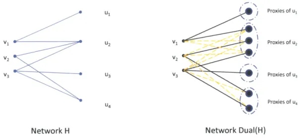
The local broadcast problem, in its full generality, assumes that different processes can keep re-ceiving broadcast requests (i.e., messages to be broadcast to their neighbors) as time continues. This describes the practical reality of contention management, which is an ongoing process. Our algorithm works in this general setting. To present the core of our lower bounds in a cleaner format, we use a simplified setting which we call the single-shot setting: the network is a bipartite network composed of two sides, called senders and receivers. Each sender has a message (from the start) and it has to deliver it to all of its receiver neighbors in the reliable part of the network. Therefore, in particular, this single-shot setting does not include an environment (which generates broadcast requests continuously). This setting is significantly simpler than the general ongoing case of the local broadcast problem, which we call the multi-shot setting. Thanks to this single-shot setting, we are able to present the core of our lower bounds away from the complications needed for the generality of the local broadcast problem. We later show that these lower bounds carry over to the multi-shot setting. Having this in mind, the organization of the main body of the thesis is divided into two parts: Part I, where we present the simplified single-shot setting and the related lower bounds, and Part II, where we present the general multi-shot setting and the related upper and lower bounds.
The more specific organization of the thesis is as follows. We start with presenting some mathematical notations and basic probabilistic inequalities in Chapter 2. These are used in both parts of the thesis. Then, the rest of the thesis is divided into two parts:
" Part I: In Chapter 3, we present the models that we use for the single-shot setting. Chapter 4 presents the statement of the local broadcast problem in this setting and the measures that we use for analyzing the performance of the related algorithms. Chapters 5 and 6 presents our lower bounds for the single-shot setting of the classical and the dual graph models, respectively.
8 presents the statement of the local broadcast problem in the multi-shot setting and the
measures that we use for analyzing the performance of the related algorithms. In Chapter 9,
we present the related work. In Chapter 10, we present our local broadcast algorithm for both
the classical and the dual graph models of this general setting. In Chapter 11, we explain
how the lower bounds of the single-shot setting, presented in Chapters
5
and 6, extend to the
general multi-shot setting.
Chapter 2
Mathematical Preliminaries
In this chapter, we define the notations used throughout this thesis and we also review some prob-ability inequalities.
2.1
Notations
"
We use the notations R and R+ to denote the set of real numbers and the set of positive real numbers, respectively. We also use the notation N to denote the set of all positive integers. * We use the notation [r, r'], for integers r and r' > r, to indicate the sequence {r, ... , r'}. Wealso use the notation [r] for integer r to indicate [1, r].
" We use the notation 2s to denote the power set of set S, i.e., the set of all subsets of S. " We use the notation Es to denote the set of all finite length sequences over set S, i.e.,
se-quences {ak}kGN such that for each i E [1, k], a, E S.
" For a graph H = (V, E), for each node u E V, the notation AH(u) describes the set of
neighbors of u in H. Moreover, we define + W(u) =
NH(u)
UU4-" We use symbols I and T to indicate two special values. These special values respectively
indicate silence and collision. For example, transmitting I means remaining silent. We explain the meaning and the usage of these symbols in Section 7.4. We use M to denote the set of all messages and we assume that M
n
{L, T} =0.
We use notations M and MITto denote sets M U {IL} and M U {I, T}, respectively.
* We use the notation w.h.p. (with high probability) to indicate a probability at least 1 - , where n is the number of the nodes in the network. We present the details of the graph model of the network in Section 7.1
2.2
Some Probability Inequalities
Theorem 2.2.1 (Union Bound). For any probability space and arbitrary events 1, 2, , Ek in this space, we have
k k
Pr[U E ]
P[i]
i=1 i=1
Theorem 2.2.2 (Chernoff Bound). Let X 1, X 2, . , Xk be independent Poisson trials such that
for each i
E
[1, k], Pr[Xi = 1] = pi, where pi E (0, 1). Let X =Z
Xj, and y = E[X]. For any 6 > 0, we havePr[X > (1+6)p1]
<
e-and
Pr[X
<
(1-6)pu]
<e- 2Next, we present a theorem by Fortuin, Kasteleyn, Ginibre, commonly referred to as the FKG inequality [7, Chapter 6], and a simple corollary of it which we use to prove Theorem 5.2.1. We start by presenting some definitions.
Definition 2.2.3. A finite lattice (L, -L) is a finite set L partially ordered by <L, in which every two
elements x, y G L have a least upper bound, denoted by xV, and a greatest lower bound, denoted
x A y. A lattice (L, <L) is distributive iffor all x, y, z E L, we have x A (y V z) = (x A y) V (x A z).
Definition 2.2.4. Suppose (L, < L) is afinite lattice. A
function
f : L
-* R is called non-decreasing(resp., non-increasing) with respect to <L if x -L y implies f (x) < f (y) (resp., if x <L y implies f(x) > f (y)).
Definition 2.2.5. Suppose (L, < L) is a finite lattice. A function p : L -+ R+ is called
log-supermodular iffor all x, y E L, we have p(x)p(y) < p(x A y)pi(x V y).
Theorem 2.2.6 (FKG Inequality). Let (L, L) be a finite distributive lattice and let Y : L -+ R+
be a log-supermodular function. If
f,
g L -* R are both non-decreasing functions with respect to -L, then we have( f W g xpW -' ( x) ;> ()
fxpW
/- ) ( g Wx/px))xcL xEL xEL xEL
Corollary 2.2.7. Consider an arbitrary integer K > 0 and suppose that A1 to At are f fixed arbitrary subsets of set [K]. Choose a subset B C [K] as follows: for each k E [K], include k in set B independently with probability p E [0,1]. We have
Proof We first show that for each
j
E [2, f], we havePr Aj
n B# 0 Vi E [1J
-1],AinB #
0
>Pr[A
nB# 0]
Let L be the set of all subsets of [K] ordered by inclusion, i.e., for each two subsets S, S' C
[K], we have S <L S' iff S C -'. With this order, for each two subsets S, S' C [K], we
have S A S' = S U S' and S V S' = S
n
S'. Thus, for each three subsets S, S', S" C [K],S A (S' V S") S u (S' n S") = (S U
S')
n (S U S") = (S A S') V (S A S"), which shows thatL with the given order is a distributive lattice. Consider the function p : L -+ [0, 1] where for any
S C [K], we have p(S) = p|S|(i _ p)K-IS|. It is easy to check that p is log-supermodular. That is
because, for each two subsets S, 5' C [K],
p'( S)p(S') = (pIS|( _ P)K-|S|) (|S'|l _ p)K-|S'|) _ |S|+|S'| p)2K-|S|--S'
= p lS+13'-| S nS'|P ssi . (1 _ )K- (S|+S'l-|SnS'I)(i - )K-(ISnS'I)
= (p|SUS'l(I _ P)K-(ISUS')) (PSnS'l 1 _ P)K-(ISnS')
=
p(S
U S')p,(S n S') =t(S
A S')p(S V S')Note that the function p is chosen such that p(S) = Pr[B = S].
Now, fix any
j
E [2, f] and consider indicator functionsf,
g : L - {0, 1} as follows: for eachset S C [K],
f(S)
= 1 iff S n Aj#
0 and g(S) = 1 iff Vi E [Ij - 1], we have Ai n B#
0.Clearly,
f
and g are both non-decreasing with respect to the inclusion order. With these definitions, it follows from the FKG inequality (Theorem 2.2.6) thatPr Vi E [1,
],
Ai n B#
0 - 1 = ( fxgx)x EL xcEL
;
f(x)p(x)).(Eg(x)p(z))
=Pr[AnB
# 0].Pr
Vi
[1,j -1],
A n B
#01
xeL xEL
Now dividing the two sides by Pr
Vi
E [1,
j
-1],A nB
#
0]
we haveGiven this inequality for any j E [2, f], we can complete the proof of the corollary easily as follows:
Pr
[Vi
# 0
fPr[A1 nB
#
0] -
Pr [A
j=2-nB
0 Vi E[1,j
f-
1],Aj
n B
#
0
>
Pr[AnB#0|-
1Pr[AjnB#0]=
Pr[AjnB#0]
j=2 j=1
F-1
E [1, f], Ain B
Part I
The Simplified Single-Shot Setting and
Lower Bounds
Chapter 3
The Models in The Single-Shot Setting
In this chapter, we present the definitions of the models that we use for the simplified single-shot setting. We use almost the same models in the second part of the thesis when studying the general multi-shot case of the problem, with the exception of a small number of changes which we briefly mention in this chapter and we explain in detail in Chapter 7.
As mentioned in the introduction, we use two models, namely the classical radio network
model (also known as the radio network model) and the dual graph model. The former model has
been extensively studied since the late 1980s [19]-[29], [31, 36, 40] and assumes that all connec-tions in the network are reliable. The latter model was introduced recently in 2009 [31, 33], and is more general in that it includes the possibility of unreliable edges. Since the former model is simply a special case of the latter, we use the dual graph model for defining both models, and also when describing the problem statement in the next chapter. However, in some places, we indicate how a certain result or property changes when we focus on the special case of the classical radio
network model.
In the dual graph model of the single-shot setting, a distributed system is composed of a set of processes that are connected to each other via a network, and an adversary that controls the commu-nications on this network to a certain extent (to be explained in Section 3.3). The main difference between this model and the model for the multi-shot setting that we explain in Chapter 7 is that, in the multi-shot version, the distributed system also includes an environment. This environment is an abstraction of the higher levels of the wireless nodes that interact with the local broadcast module (abstracted as processes here). In Chapter 7, we present the details of the definition of the environment and explain the interactions between the environment and the processes.
The rest of this chapter is organized as follows: In Section 3.1, we present the network connec-tion assumpconnec-tions for the dual graph model. We explain what a process in this model is in Secconnec-tion
3.2. In Section 3.3, we explain how a distributed system in the single-shot setting works as a whole,
all Sections 3.1 to 3.3, we try to present the model as general as possible, in order to keep it similar to its counterpart in the multi-shot setting (Chapter 7). However, in our lower bounds (all results in Chapters 5 and 6), we use a stronger model, centralized setting, which we explain in Section 3.4.
3.1
Network Connections
In the dual graph model, radio networks have some reliable links and potentially some unreliable links. In the dual graph model, we define a network (G, G') to consist of two undirected finite graphs, G = (V, E) and G' = (V, E'), where we have E C E'. Intuitively, set E is the set of
reliable edges while E' is the set of all edges (both reliable and unreliable). We assume that the communications on the unreliable edges, i.e., the edges in set E'\E, are controlled by an adversary. We explain this issue in more detail in Section 3.3. When restricting attention to the special case of the classical radio network model, there are no unreliable edges and thus, we simply have G = G', i.e., E = E'. We define the size of the network to be n = |V1. We remark that graphs G and G'
can be disconnected.
We assign processes to graph nodes of the network (G, G'). This assignment is defined by an injective function idO from V to the set of process ids [N] (refer to Section 3.2 for process definitions.). That is, for each v E V, id(v) indicates the id of the process assigned to graph node
v. For each v E V, we use notation proc(v) to indicate the process with id id(v), i.e., the process
that is assigned to graph node v. We sometimes abuse notation by using the notation process u, or sometimes just u, for some graph node u E V, to refer to proc(u). We refer to a network (G, G')
and a mapping idO from graph nodes to processes as a setting.
Processes can potentially know the network (G, G') or have some partial knowledge about it'. This means that processes could have a full description of the network or some information about it built into their states, and the related distributed algorithm is required to work only if this full description matches the description of the network or if this partial information is consistent with the description of the network. To strengthen our results, we remark that lower bounds (all results in Chapters 5 and 6) allow full knowledge of the network graphs (G, G').
3.2
Distributed Algorithms and Processes
We define a distributed algorithm A to be a collection of N randomized processes, where N is an arbitrary positive integer. Processes are described by probabilistic automata and intuitively, in each process, we have two types of transitions: (1) probabilistic transitions that take the state at the
'This is because, in many real world settings, it is reasonable to assume that devices can make some assumptions or inference about the structure of the network.
beginning of a round to an intermediate state and a message to be transmitted on the channel (or silence), (2) deterministic transitions that take an intermediate state and a message received from the channel (or a special value _ or T) to the state at the end of a round.
The formal definition of processes is as follows: Each process in A is a 6-tuple (i, Qi, P', SO, TFi,)
and we have:
*
i E [N] is the unique identifier of this process.*
Qi
and P" are two sets of states, and we have Qin
Pi =0.
We refer to states in these two sets respectively as Q-states and P-states.* So E Qi is a single starting state.
" T is a function that captures the probabilistic transitions of the process. For each state
S E
Q',
function FT(S) : P' xM
1 - [0, 1] is a probability distribution function over P' xM
. That is, for each state S' E Qi, and each m EM
,F(S)(S',
m) is theprobability that, given that the process with id i is in state S, it makes a transition to state
S' and transmits m if m
#
I and remains silent if m = 1. Note that, as mentioned in Section 2.1, in this notation, symbol I means remaining silent.* 9' :
P' xMj-
1-
-Q'
is a function that captures the deterministic transitions of the process.For each state
S' E
P' and eachm'
E MTI,gl(S', M')
is a state inQi,
and we have the following: if the process with id i is in P-state S' and it receives m' from the channel, then it makes a transition to stateg(S',
m').For simplicity, we sometimes use process i to refer to the process with id i.
3.3 Executions in the Dual Graph Model
As mentioned at the start of this chapter, in a distributed system in the dual graph model, a set of processes are connected to each other via a network as described in Section 3.1, where the communications over this network are controlled by an adversary. In this section, we explain how this system works as a whole by describing the executions of a distributed algorithm in this model and explaining the role of the adversary. An execution of an algorithm A in network (G, G') proceeds as follows:
The execution proceeds in synchronous lock-step rounds 1, 2, ..., where all the participating processes start in the first round. At the start of each round r, every process proc(u), u E V is in a state S E Qi, where i = id(u). In particular, at the start of the first round, proc(u) is in state
S' E Pi, and it also determines a value m E ML. If m' / 1, then proc(u) transmits message m' in round r. Otherwise (i.e., if m' f 1), proc(u) remains silent in round r. That is, as explained in Section 3.2, choosing m' = I during this transition means that process i remains silent in round r. Next, the adversary chooses a reach set that consists of E and a subset, potentially empty, of edges in E' - E. This reach set potentially affects what message (or value I or T) each process receives. Intuitively, this reach set describes the links that are active in this round. We emphasize that when focusing on the special case of the classical model, set E'- E is empty and therefore, the reach set is just E. In the dual graph model, we assume that the adversary is 'adaptive offline' [8] meaning that it has full knowledge of the history of the execution and in particular the state of the network when it is determining the reach sets. This means that when choosing the reach set of round r, the adversary knows everything that happened up to round r of the execution including the outcome of the random coins used for the transition of round r. In particular, the adversary knows which processes are transmitting in round r. Moreover, we assume that the adversary can also make randomized decisions.
After the adversary determines the reach set of round r, depending on this reach set and which processes are transmitting, each process i receives exactly one value in set MI from the channel. For a graph node v, let Bv,, be the set of all graph nodes a such that proc(u) transmits in r and edge e = {u, v} is in the reach set for this round. What proc(v) receives in round r is determined by the following rules:
(A) If proc(v) broadcasts in round r, then it receives only its own message.
(B) If proc(v) does not broadcast, and
IB,,,
= 0 or |B,,, > 1, then proc(v) receives I(indi-cating silence).
(C) If proc(v) does not broadcast, and |Bv,, 1, then proc(v) receives the message sent by
proc(u), where u is the single node in B,,r.
The rule (A) intuitively means that each process cannot send and receive simultaneously. We remark that the rule (B) means that we do not assume any collision detection mechanism in this model. To strengthen our results, we present our lower bounds (all results in Chapters 5 and 6) in the stronger model with collision detection, i.e., where the rule (B) is replaced with the following rule
(B') If proc(v) does not broadcast, and
IBvrI
= 0, then proc(v) receives 1. If proc(v) does not broadcast, and |B,,,I > 1, then proc(v) receives T (indicating collision).After receiving the messages of round r, every process proc(u), u E V makes its deterministic
P-state S' E P', where i
=
id(u) and it receives m' EAIT from the channel. Then proc(u)makes a transition to Q-state
gi
(S', in'). We remark that at the end of each round, the state of thewhole system consists of just Q-states for all processes.
3.4
Centralized Setting For Lower Bounds
In our lower bounds (all results in Chapters 5 and 6), we consider the stronger model of
central-ized algorithms. We define a centralcentral-ized algorithm to be the same as the distributed algorithms
explained in this chapter, with two modifications: (1) the processes know the graph (G, G') and the mapping id() from the beginning of the execution; and (2) when the processes are making their transitions, they know the full history of the execution and thus, their transitions are a function of the full history of the execution. This history in particular includes the current state of all the processes in the network.
Finally notice that in the centralized setting, since each process knows the full history of the execution, in each round r, each process knows exactly which set of its neighbors transmitted. Thus, each process knows whether zero or two or more of its neighbors transmitted in that round. Thus, in the centralized setting, the models with and without collision detection are equivalent.
Chapter 4
The Local Broadcast Problem in The
Single-Shot Setting
The intuitive description of the local broadcast problem in the single-shot setting is as follows: The nodes of the network are divided into two groups, the senders and the receivers. Moreover, no two senders are neighbors and no two receivers are neighbors. The objective of the problem is that, each sender should deliver a special message that it has to all of its receiver neighbors. In this chapter, we present the formal definition of this problem, and present the time bounds that we use to measure the performance of the algorithms that solve this problem.
4.1
The Local Broadcast Problem
In this single-shot setting, the processes, the network and the executions are as presented in Chap-ter 3. In the version of the local broadcast problem tailored to this setting, we moreover have:
1. The network (G, G') consists of two undirected finite bipartite graphs, G = (V, E) and G' = (V, E'), where we have: V = S U R,
S nR =
0, |SI > 1, |RI ;> 1, |V| = n, andE C E'. Moreover, each edge e E E' is an unordered pair {v, u} such that v E S and u E R.
The nodes in sets S and R are respectively called the senders and the receivers. Moreover, the processes assigned to the sender nodes and the receiver nodes are respectively called the
sender processes and the receiver processes.
2. Each process i has one special message mi E M (encoded in all of its states, and particularly its starting state So) and for each i,
j
E N such that i$
j,
we have mi#
n.3. Each process i has a boolean variable acki E {False, True} (in each of its states). In starting state Si, we have acki = False. Each process i can change the value of variable
acki at most once and thus, only from a False value to a True value. Moreover, this change
can only happen during a transition from a P-state to a Q-state (the second transition of a round). Formally these two conditions mean that (1) there is no transition from a Q-state
Q
to a P-state P such that the value of acki in statesQ
and P is different, and (2) there is no state transition from the P-states in which acki = True to the Q-states in which acki = False.The informal description of the local broadcast problem in this setting is that for each sender node v E S, process proc(v) should eventually deliver special message mi, where i = id(v), to all of its receiver G-neighbors, with high probability. This is formalized as follows: We say that an algorithm A solves the local broadcast problem provided that, when A operates in any dual graph
(G, G'), we have:
(A) In every execution, for each sender node v E S, process proc(v) eventually sets acki =
True, where i = id(v).
(B) For each particular sender node v E S and each round r, if process proc(v) has acki = True,
where i = id(v), at the end of round r, then with high probability, for each (receiver) node
u E JVG(v), process proc(u) has received message mi by the end of round r. Here, the probability space is based on all the probabilistic choices of the algorithm and the adversary. Moreover, the probability distribution in this requirement is conditional on the event that
proc(v) has acki = True at the end of round r.
An algorithm A that solves the local broadcast problem is called a local broadcast algorithm.
4.2
The Time Bounds
We measure the performance of a local broadcast algorithm by two bounds: the acknowledgment
bound and the progress bound. For any given local broadcast algorithm A and any fixed single-shot
setting (G, G'), these bounds are defined as follows:
1. A number t E N is an acknowledgment bound for A in (G, G') if for each sender process
proc(v), at the end of round t, with high probability, proc(v) has acki = True, where
i = id(v).
2. A number t E N is a progress bound for A in (G, G') if for each receiver process proc(u) such that node
NG
(u)I
> 1, with high probability, proc(u) has received at least one special message mi for an i such that process i = id(v) and v E XG(v), by the end of round t.In the following lemma, we show that progress bound is less than or equal to acknowledgment bound. The formal statement is as follows:
Lemma 4.2.1. For any local broadcast algorithm A, any single-shot setting (G, G'), and any
r E N, if T is also an acknowledgment bound for A in (G, G'), then T is a progress bound for A in
(G, G').
Proof Consider an arbitrary local broadcast algorithm A, a single-shot setting (G, G'), and a
T E N such that r is an acknowledgment bound for A in (G, G'). Following the definition of
acknowledgment bound, we get that in each execution of A, by the end of round r, for each sender process with id i we have acki = True. Moreover, following the definition of the local broadcast
problem, we get that in executions of A, by the end of round T, with high probability we have that
each receiver process proc(u) has received the special message mi, for every i such that i = id(v)
and v E KG(u). Thus, by the end of round r, with high probability, we have that each receiver process proc(u) such that node
ING(u)|
;> 1 has received at least one special message mi for an i such that process i = id(v) and vc
JG(U). Comparing this with the definition of progress boundshows that T is a progress bound for A in (G, G'). D
The acknowledgment and the progress time bounds defined above often depend on the maxi-mum contention of the network, which is defined as follows:
Definition 4.2.2. In the single-shot setting, the maximum contention A' (resp., A in the classical
model) is equal to the maximum G'-degree (resp., G-degree in the classical model) of the receiver nodes.
We sometimes use the phrase the maximum receiver degree instead of the maximum contention. The definition of the maximum contention in the multi-shot setting has similarities to this defini-tion, but is more complicated and requires careful definitions for the amount of contention in each round and for each node. We present that definition in Chapter 8.5.
Chapter
5
Lower Bounds in the Classical Radio
Broadcast Model
In this chapter, we focus on the problem of local broadcast in the single-shot setting of the classical model (for formal definitions of this setting, refer to Chapters 3 and 4). We present lower bounds for both the progress and the acknowledgment time bounds. We emphasize that all these lower bounds are presented for centralized algorithms and also, in the model where processes are pro-vided with a collision detection mechanism. Note that these points only strengthen these results.
In Chapter 11 we explain that since the single-shot setting can be viewed as a special case of the multi-shot setting, these lower bounds extend to the multi-shot setting as well. Thus, they prove that the optimized decay protocol for the general multi-shot setting, which we present in Chapter 10, is optimal with respect to progress and acknowledgment times in the classical model. These lower bounds also show that the existing constructions of Ad Hoc Selective Families [27, 28]
are optimal. Moreover, in Chapter Chapter 6, we use the lower bound on the acknowledgment time in the classical model that we present here as a basis for deriving lower bounds for progress and acknowledgment times in the dual graph model.
5.1
Progress Time Lower Bound
In this section, we remark that, following the proof of the Q(log2 n) lower bound of Alon et al.
[21] on the time needed for global broadcast of one message in radio networks, and with slight modifications, one can get a lower bound of Q(log A log n) on the progress bound in the classical model.
Theorem 5.1.1. For any sufficiently large n and any A < n, there exists a single-shot setting in
A, such that for any local broadcast algorithm, the progress bound in W(n, A) is greater than
Q(log A log n) rounds.
Proof Outline. The proof is an easy extension of [21] to networks with maximum contention A.
This proof uses the probabilistic method [7] to show that such a network N(n, A) exists. The only change from [21] is that instead of choosing the receiver degrees to vary between n04
and no6, we choose the degrees between e(A1/4)
and E(A1
/2). This leads to E(log A) (instead of 8(log n))
different classes of degrees, and in turn, to the stated bound. The rest of the proof remains the same as in [21].
5.2
Acknowledgment Time Lower Bound
In this section, we present our lower bound on the acknowledgment time in the classical radio broadcast model.
Theorem 5.2.1. For any sufficiently large n and any A E [20 log n, n0
-1], there exists a single-shot
setting in the classical model with a bipartite network H (n, A) of size n and maximum contention of at most A, such that the acknowledgment bound of any algorithm in H (n, A) is greater than
Alogn rounds. -00
In the proof of this theorem, instead of showing directly that randomized algorithms have low success probability, we show a stronger variant, by proving an impossibility result: In Lemma 5.2.2, we prove that there exists a single-shot setting with a bipartite network H (n, A) of size n and max-imum contention at most A in which, even with a centralized algorithm, it is not possible to sched-ule transmissions of nodes in at most A log rounds such that each receiver receives the message of
100
each of its neighboring senders. In particular, this result shows that in H (n, A), for any randomized local broadcast algorithm, the probability that in at most Alogn rounds, each receiver receives the
100
message of each of its sender neighbors is zero. In proof of Theorem 5.2.1 (presented at the end of this section), we argue that this means that no local broadcast algorithm has an acknowledgment bound of at most Alogn in H(n, A).
100
To present Lemma 5.2.2, we first present some definitions. A transmission schedule 0 of length
L(a) for a bipartite network is a sequence O1, .. . , oL
C
S of sets of senders. Having a senderu E or indicates that at round r the sender u is transmitting its message. For a network G, we say that transmission schedule a covers G if for every u E R and every v E
NAG(u),
there exists a round r such that orn
NG(u)
= {v}, that is, using transmission schedule a each receiver nodereceives the message of each of its sender neighbors. Now we are ready to see the main lemma which proves our bound.
Lemma 5.2.2. For any sufficiently large n and any A
E
[20 log n, no-'], there exists a single-shotsetting with a bipartite network H (n, A) with size n and maximum receiver degree at most A,
for which there does not exist a transmission schedule o such that L(u) < A 100"o9n and a covers
H (n, A).
We next present the proof of Lemma 5.2.2. As in the previous section, our proof uses tech-niques similar to those of [20, 21, 22] and utilizes the probabilistic method [7] to show the existence of the network H (n, A) mentioned in Lemma 5.2.2.
Proof Outline. First, we fix a sufficiently large n and A E [20 log n, no'] and let q no-12 and qt = 1q8 - no.9 6. Note that if n is sufficiently large, we have 20 log n < n0. Next, we present a
probability distribution over a particular family
g
of bipartite networks. The common structure of this graph familyg
is as follows. All networks ofg
have a fixed set of nodes V. Moreover, V is partitioned into two nonempty disjoint sets S and R, which are respectively the set of senders and the set of receivers. We have |SI = y and |RI = n - q. Note that for any sufficiently large n, wehave |RI =n- n 2 > 7.9 Ti', 7 where the inequality holds because n is sufficiently large. In order to define the probability distribution of these graphs, we describe the process that chooses a random network from
g.
We create a random network fromg
by independently puttingan edge between any s E S and r E R with probability A.
We use the following definitions. Let BAD1 be the event in the probability space of graphs
that the maximum receiver degree of the graph G E
g
is greater than A. For each transmission schedule o, call o short if L(u) < A4ogf. 100 Let BAD2 be the set of graphs G Eg
such that thatthere exists a short transmission schedule that covers G.
We first show in Lemma 5.2.3 that Pr[BADI] < -L. Then we show in Lemma 5.2.4 that Pr[BAD2] < W. A union bound then shows that with probability at least 1 - > 0, neither of the
two events BAD1 and BAD 2 happen. This means there exists a graph in
g
that has the maximumreceiver degree at most A and no short transmission schedule covers it, and thus completes the
proof. E
Lemma 5.2.3. Pr[BAD1] < 1
Proof We show that the probability that the maximum receiver degree of a random graph G C
g
is greater than A is at most -. For each receiver r E R, let XG(r) denote the degree of receiver r in graph G E
g.
Then, E[XG(r)] =$.
Moreover, since edges are added independently, we can use a Chernoff bound (Theorem 2.2.2) and obtain that Pr[XG(r) > A] < e-. Using a union bound over all choices of receiver node r, and noting that |RI < n and A > 20 log n, wecomplete the proof as follows:
Pr[-r
(E
R s.t.XG (r) > A] re 6 <lo n-6 < e "- " = e- logn <nD
Lemma 5.2.4. Pr[BAD2] < 12n
Proof Outline. For each transmission schedule a, let E, be the event in the probability space of
graphs that o covers graph G
c
g.
Also, let us denote the set of all short transmission schedules byS-ORT. Having these definitions, the probability that there exists a short transmission schedule
a that covers G E
g
is Pr[UaGSWOT E]. That is, Pr[BAD2] = Pr[Uo-ESHORT E]. Thus, usinga union bound, we can infer that Pr[BAD21 <
EES-oyZT
Pr[E,]. Having this inequality inmind, we first show in Lemma 5.2.5 that for each a E S7ORT, Pr[E,] e-"" 2. Then, we
show in Lemma 5.2.7 that |SRORTI < 24"' . At the end, we use the inequality Pr[BAD2] 5
Z.ESO'RT Pr[E,] along with Lemmas 5.2.5 and 5.2.7 to complete the proof. El Lemma 5.2.5. For each a
E
S7ORT, Pr[E,] < e-nProof Fix an arbitrary short transmission schedule a. For each round t of a, let N(t) denote the
number of senders that transmit in round t. Also, call round t an isolator if N(t) = 1. For each sender s E S, if there exists an isolator round in o- where only s transmits in that round, then call sender s lost. Since L(o-) < Alogn < 1
o" < n 012 = I, there are at least - senders that are not
10- 100 2 2' 2
0o.1 log n __12
lost. We remark that inequality ""100 < n holds because n is sufficiently large.
For each not-lost sender s, we define a potential function <D(s) = N where T, is the set of rounds in which sender s transmits. Note, that for each round t, the total potential given to not-lost senders in that round is at most N(t) - 1= 1. Hence, the total potential when summed
over all rounds is at most Alog" 100 - 12 2Alog , Therefore, since there are at least - not-lost senders,
2
there exists a not-lost sender s* for which <D(s*) < g For the rest of the proof, fix a non-lost sender s* such that <D(s*) < A . Now we focus on sender s* and rounds T,.. We show the following claim:
Claim 5.2.6. For each receiver r E R, the probability that receiver r is a neighbor of s* and it
does not receive the message of s* is at least
Proof Consider an arbitrary receiver r. For each round t E T,-, we say receiver r is blinded in
round t if r is connected to at least one sender node other than s* that transmits in round t. Having this definition, the proof of Claim 5.2.6 is based on two facts as follows:
(F1) Pr [r is a neighbor of s*] = A ' > .
(F2) Pr [Vt G T,., r is blinded in round t] .
In order to prove fact (F2), we use the FKG inequality [7, Chapter 6] and particularly its simplified form presented in Corollary 2.2.7. In particular, in this application of Corollary
2.2.7, set [K] is the set of senders other than s*, the set B is the set of sender neighbors of
receiver r other than sender s*, p = , f = |Ts-|, and the A set are: for each round t E Ts.,
we have one set Ai which is equal to the set of all senders other than s* that transmit in round t. Thus, using Corollary 2.2.7, we get that
Pr[Vt E Ts., r is blinded in round t] >
17
Pr[r is blinded in round t].t ETs*
Now for each t E Ts., we have
Pr[r is blinded in round t] = 1 - (1 - A)N(t) 1 - (N(t)-1)
M (t) (M 4,1 1
>1 e N(t) -> N(t)
where inequality (t) holds because N(t) > 2 as s* is not-lost, and inequality
($)
holds as for any x > 0, we have e-x + e-lx < 1. Hence, we havePr[Vt G Ts., r is blinded in round t] > fj Pr[r is blinded in round t]
t c
s
t ET'By choice of s*, we have <b(s*) < A . Thus,
Pr[Vt E T8., r is blinded in round t] > e- >'s') e-41g
(-2/3
log n logNow note that whether r is connected to each sender other than s* is independent of whether it is connected to s*. Thus, the two events considered in parts (Fl) and (F2) are independent. Hence, for each receiver r, the probability that r is a neighbor of s* and in each round t E Ts*, r is blinded is at least - = -. This means that the probability that r is a neighbor of s* but it never receives the message of s* is at least -L. This completes the proof of Claim 5.2.6. El
7
Now we use Claim 5.2.6 to complete the proof of Lemma 5.2.5. Since edges of different receivers are chosen independently, we get that the probability that there does not exist a receiver r