Publisher’s version / Version de l'éditeur:
ASHRAE Transactions, 115, 2, pp. 1-20, 2009-06-01
READ THESE TERMS AND CONDITIONS CAREFULLY BEFORE USING THIS WEBSITE. https://nrc-publications.canada.ca/eng/copyright
Vous avez des questions? Nous pouvons vous aider. Pour communiquer directement avec un auteur, consultez la
première page de la revue dans laquelle son article a été publié afin de trouver ses coordonnées. Si vous n’arrivez pas à les repérer, communiquez avec nous à [email protected].
Questions? Contact the NRC Publications Archive team at
[email protected]. If you wish to email the authors directly, please see the first page of the publication for their contact information.
NRC Publications Archive
Archives des publications du CNRC
This publication could be one of several versions: author’s original, accepted manuscript or the publisher’s version. / La version de cette publication peut être l’une des suivantes : la version prépublication de l’auteur, la version acceptée du manuscrit ou la version de l’éditeur.
Access and use of this website and the material on it are subject to the Terms and Conditions set forth at
Thermal modeling of shading devices of windows
Laouadi, A.
https://publications-cnrc.canada.ca/fra/droits
L’accès à ce site Web et l’utilisation de son contenu sont assujettis aux conditions présentées dans le site LISEZ CES CONDITIONS ATTENTIVEMENT AVANT D’UTILISER CE SITE WEB.
NRC Publications Record / Notice d'Archives des publications de CNRC:
https://nrc-publications.canada.ca/eng/view/object/?id=3860826a-999e-4532-a06b-35c0cab3b6bc https://publications-cnrc.canada.ca/fra/voir/objet/?id=3860826a-999e-4532-a06b-35c0cab3b6bc
http://irc.nrc-cnrc.gc.ca
T he r m a l m ode ling of sha ding devic e s of
w indow s
N R C C - 5 1 1 2 1
L a o u a d i , A .
J u n e 2 0 0 9
A version of this document is published in / Une version de ce document se trouve dans:
ASHRAE Transactions
, 115, (2), pp. 1-20
The material in this document is covered by the provisions of the Copyright Act, by Canadian laws, policies, regulations and international agreements. Such provisions serve to identify the information source and, in specific instances, to prohibit reproduction of materials without written permission. For more information visit http://laws.justice.gc.ca/en/showtdm/cs/C-42
Les renseignements dans ce document sont protégés par la Loi sur le droit d'auteur, par les lois, les politiques et les règlements du Canada et des accords internationaux. Ces dispositions permettent d'identifier la source de l'information et, dans certains cas, d'interdire la copie de documents sans permission écrite. Pour obtenir de plus amples renseignements : http://lois.justice.gc.ca/fr/showtdm/cs/C-42
Thermal Modeling of Shading
Devices of Windows
A. Laouadi, Ph.D., ASHRAE member
Institute for Research in Construction, National Research Council of Canada 1200 Montreal Road, Building M-24, Ottawa, Ontario, Canada K1A 0R6
Tel.: (613) 990 6868. Fax: (613) 954 3733. Email: [email protected]
ABSTRACT
Shading devices are important design elements of glazed façades to reduce energy consumption of buildings and improve thermal and visual comfort of occupants. Although there has been significant development in the evaluation and modeling of the thermal performance of shading devices, current methodologies are limited to a few shading products and types. Furthermore, current fenestration thermal models do not account for radiation emission and absoption throughout shading layers, and elemements for energy generation and conversion imbedded in glazing layers. This paper presents a general methodology to compute the thermal performance of fenestration systems incorporating permeable shading devices and elements for energy generation and conversion. The methodology assumes each shading layer as porous with effective radiation and thermal properties. The effective properties account for the geometrical and thermal characteristics of the shading layer, and the effect of the convective heat transfer within the layer porous structure. Using the concept of the thermal penetration length, effects of porous shading layers on the convective heat transfer from their boundary surfaces to the adjacent gas spaces are also accounted for. A validation study is carried out, in which the U-factor of a double-glazed window with between-pane Venetian blinds are compared with the available laboratory measurement. The comparison results show that the model predictions are in good agreement with the measurement.
INTRODUCTION
Shading devices are important design elements of glazed façades to reduce energy consumption of buildings and improve thermal and visual comfort of occupants. Shadings may be placed between glazing layers, or attached to the interior or exterior façade surfaces to control natural illumination, solar heat gains, glare, view out, heat loss through facades. In some applications of double skin facades, shading devices are used to manage energy flows to/from buildings. Most popular types of shading devices include slat-type blinds, roller screens and draperies. Although there have been significant advancement in the performance evaluation of shading devices, predictions of their thermal performance remain a challenge to be addressed due to their complex geometries and effect on the heat transfer mechanisms.
In the past decades, there has been significant work devoted to the evaluation of the optical, daylighting and energy performance of shading devices. The ISO standard 15099 (ISO, 2003) presents a validated model to compute the optical and long-wave radiation characteristics of slat-type blinds. The IEA Task 27 (Kohl, 2006) carried out a comprehensive assessment of the solar optical and thermal performance of several product types of interior and exterior blinds and roller shades through measurement and computer simulation using the ISO-like and simple models. The IEA Task 34/43 (Loutzenhiser et al., 2007) carried out empirical validations of building-energy simulation tools for daylighting performance and thermal loads of interior and exterior Venetian blinds and shading screens. Most of the tested simulation tools used simple models for the prediction of the optical and thermal performance of the shading devices.
However, models to predict the thermal performance (e.g., U-factor) of fenestration systems incorporating shading devices are at the early stage, particularly those related to convection flows in open gas cavities adjacent to permeable shading layers. The current methodology is based on the thermal-resistance approach developed for simple fenestration systems, made up of essentially thermally opaque
glazing (ISO, 2003; Wright, 2008). A one-dimensional conduction heat transfer model is used for glazing layers coupled with radiation and convection models at the layer boundary surfaces. Radiation emission is assumed at the boundary surfaces of layers. Convection models use the existing correlations for the convective film coefficients in gas cavities or around flat surfaces. Complex shading layers are treated as individual layers with effective radiation properties, but with assumed uniform layer temperature (no thermal resistance of shading layer). These simple models have been implemented in currently available fenestration tools such as WINDOW (LBNL, 2008) and WIS (WinDat, 2008). Recent research showed, however, that these simple models were not accurate for slat-type blinds (Yahoda and Wright, 2004a), and for diathermanous - infrared transparent- layers (Collins and Wright, 2006). Furthermore, these models do not account for elements imbedded in glazing layer for energy generation and conversion, which are getting more popular in today’s high performance building designs.
Due to the limitations of existing prediction models of shadings, ASHRAE has sponsored a research project (RP 1311) to develop validated optical and thermal prediction algorithms for several types of shading devices, including slat-type blinds, drapes, roller blinds and insect screens (Kotey et al., 2009a,b). For the purpose of validation studies, Garnet (1999) and Huang (2005) conducted laboratory measurement using the guarded heater plate apparatus of the U-factor of clear and low-e double-glazed windows with between pane metallic Venetian blinds. They found that the slat-tip-to-glazing spacing and slat angle positions had significant effect on the U-factor of the window and blind system. The thermal bridging effect of the metallic blinds reached its maximum when the slat angles were horizontal, resulting in a higher U-factor than that of closed slats. Recently, Wright et al. (2008) developed a simplified model to compute the film coefficient of a double glazed window cavity with between-pane metallic blinds. The blinds divide the window cavity into two sub-cavities. Wright et al. (2008) used the existing cavity correlations to compute the film coefficients of the sub-cavities based on a modified sub cavity width. The latter, which is larger than the true sub-cavity width (equal to slat tip-to-glazing spacing), was found proportional to the slat width and its cosine angle. The proportionality constant was determined by comparing the model predictions of U-factor with the measurement results of Huang (2005). The proposed model, termed Reduced Slat Length, yielded exceptional results for the window cavity spacings of 17.78
mm and 25.4 mm. However, the model failed to accurately-predict the U-value of the window with the larger cavity spacing of 40 mm. Despite this drawback, the model of Wright et al. (2008) indicates an important conclusion that existing correlations for cavity film coefficients may be safely used to predict the thermal performance of window and shade systems without recurring to the time-consuming and computationally intensive CFD simulations. Furthermore, the model of Wright et al. (2008) allows more flexibility to address other combinations of shading types and tilted window configurations.
CFD computer simulations have also been used for varying purposes: (1) to investigate the flow and temperature patterns in gas cavities between glazing and shading layers, (2) to validate the simulation results with the measurement, and (3) to develop useful correlations for the convective film coefficient in cavities between glazing and shading layers. Laminar, two-dimensional flows were generally considered in the investigated work. Convective flows with and without direct radiation coupling in windows with internal and between-pane Venetian blinds were addressed by several researchers, including Ye et al. (1999), Phillips et al. (2001), Collins et al. (2002a,b), Collins (2004), Shahid (2003), Shahid and Naylor (2005), Naylor and Collins (2005), Naylor et al. (2006), Avedissian (2006), and Avedissian and Naylor (2007). The maximum effect of blinds on the heat transfer through the window and blind system was found when the blinds were closed. The obtained simulation results for the temperature and flow patterns compared favourably with the available measurement of similar window and blind configurations. Correlations for the average Nusselt number of the window-blind cavity were also developed for various slat angles, and used in thermal-resistance models to compute the U-factor of window and shading systems. The predictions of the U-factor of window using such improved models compared generally well with the full CFD simulation.
It should be noted that the current advanced empirical and CFD-based thermal models are limited to single or double glazed windows with specific metallic blinds. They do not account for other thermal properties of blinds such as thermal conductivity and slat spacing. Furthermore, they cannot be applied to other types of shading devices such as drapes, or to other window tilt configurations.
The aim of this paper is to develop a general methodology to compute the thermal performance of fenestration systems incorporating shading devices for implementation in fenestration computer programs.
OBJECTIVES
The specific objectives are:
• To revisit the current models for heat transfer mechanisms through fenestration systems, and include the peculiarities of shading devices, such as permeability to mass and thermal radiation, and elements for energy generation and conversion.
• To develop models to compute the effective thermal properties of permeable shading layers. • To develop models to compute the convection film coefficients of gas spaces adjacent to
permeable shading layers.
• To validate the methodology by comparing its predictions with the available measurement.
THE PROPOSED METHODOLOGY
Shading devices make a simple glass fenestration system a far more complex system with complex heat transfer mechanisms to handle. Shading layers may be permeable to gas and thermal radiation, and the resulting cavity spaces may be open so that gas can move from one space to another. Shading layers may also emit or absorb thermal radiation throughout their media, so that local temperature gradients may be reduced compared to thermally opaque layers. Heat transfer may be further complicated if glazing layers include elements for heat generation (such as electric thin films to control moisture condensation) or energy conversion (such as photovoltaic conversion), which are getting more popular in today’s high performance building designs. Current fenestration thermal models (ISO, 2003), which are implemented in existing fenestration design tools such as Window (LBNL, 2008) and WIS (WinDat, 2008), do not account for such effects of complex fenestration systems. This section sheds some light on the heat transfer mechanisms in fenestration systems with shading devices, and develops appropriate models to compute their thermal performance.
Assumptions
The following assumptions are considered.
• Each fenestration layer is assumed solid and porous with calculated effective radiation and thermal properties to account for any convection and radiation effect in a layer medium.
• Heat transfer through a layer medium is by one-dimensional conduction.
Layer Heat Transfer
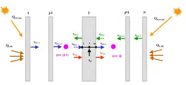
Consider a multi-layer fenestration system consisting of (N) layers as shown in Figure 1. Layer 1 faces the exterior environment and layer (N) faces the interior environment. Each layer (j) is surrounded by gaseous spaces at its boundary surfaces. The layer exchanges heat with the adjacent environments by convection to the gaseous spaces and radiation to the adjacent layers. The exchanged heat at the layer surface is then transported through the layer medium by conduction, and radiation. By virtue of the foregoing assumptions, the transient energy balance of an elemental control volume at node (i) within a layer (j) is expressed by the following relation (Siegel and Howell, 2002):
i j i j sol i j r j i j i j i j i j
q
q
q
x
T
k
x
t
T
c
, , , ,, ,, 0,, ,⎟⎟
+
+
⎠
⎞
⎜⎜
⎝
⎛
−
∂
∂
∂
∂
=
∂
∂
ρ
(1) where:cj,i : effective specific heat at node i of layer j (J/kg.K; Btu/lb.F)
kj,i : effective thermal conductivity at node i of layer j (W/m.K; Btu/h.ft.F)
qr,j,i : net radiation flux per unit surface area at node i of layer j (W/m2; Btu/h.ft2)
qsol,j,i : absorbed solar radiation per unit volume at node i of layer j (W/m3; Btu/h.ft3)
q0,j,i : heat generation per unit volume at node i of layer j (W/m3; Btu/h.ft3)
ρj,i : effective density at node i of layer j (kg/m3; lb/ft3)
If the front (facing the exterior enviroment) and back (facing the interior enviroment) surfaces of layer j are both subject to beam and diffuse incident solar radiation, the absorbed solar heat per unit volume at node i is expressed as follows:
i j sol b i j sol f i j sol q q q ,, = , , , + , , , (2) With:
(
f beam fdif)
j f i j f PV PV dif f i j d f beam f i j f i j sol f q q SR TR q q q, , , =α , , ⋅ , +α , , , ⋅ , − ⋅η ,,, ⋅ ,1: −1 , + , (3)(
bbeam bdif)
j N b i j b PV PV dif b i j d b beam b i j b i j sol b q q SR TR q q q , ,, =α , , ⋅ , +α , , , ⋅ , − ⋅η , ,, ⋅ , : +1 , + , (4) where:qf,beam : beam solar radiation flux density incident on the front surface of fenestration system
(W/m2; Btu/h.ft2)
qb,beam : beam solar radiation flux density incident on the back surface of fenestration system
(W/m2; Btu/h.ft2)
qf,dif : diffuse solar radiation flux density incident on the front surface of fenestration system (W/m2;
Btu/h.ft2)
qb,dif : diffuse solar radiation flux density incident on the back surface of fenestration system (W/m2;
Btu/h.ft2)
SRPV : ratio of photovoltaic surface area to layer surface area (-)
TRf,1:j-1 : front solar transmittance of layer stack 1 to j-1 (-)
TRb,N:j+1 : back solar transmittance of layer stack N to j+1 (-)
αf,j,i : absorption coefficient per unit length of layer j at node i for the front incident beam solar
radiation (m-1; ft-1)
αb,j,i : absorption coefficient per unit length of layer j at node i for the back incident beam solar
radiation (m-1; ft-1)
αf,d,j,i : absorption coefficient per unit length of layer j at node i for the front incident diffuse
solar radiation (m-1)
αb,d,j,i : absorption coefficient per unit length of layer j at node i for the back incident diffuse
solar radiation (m-1; ft-1)
ηPV,f,j,i : photovoltaic cell efficiency of layer j at node i to convert the front incident solar energy
into electric energy (-)
ηPV,b,j,i : photovoltaic cell efficiency of layer j at node i to convert the back incident solar energy
into electric energy (-).
The intermediate stack transmittance values (TRf,1:j-1, TRf,N:j+1) are usually not standard outputs of a
fenestration calculation program. However, they can be determined based on the standard outputs for the layer absorptances and fenestration system reflectances as follows:
∑
− = − = − − 1 1 , 1 : 1 , 1 j k k f f j f RF AB TR (5)∑
+ = + = − − 1 , 1 : , 1 j N k k b b j N b RF AB TR (6) where:ABf,j : front solar absorptance of layer j (-)
ABb,j : back solar absorptance of layer j (-)
RFf : front solar reflectance of fenestration system (-)
RFb : back solar reflectance of fenestration system (-)
The nodal solar absorption coefficients (αj,i) may be calculated based on the layer solar absorptance
(ABj). In the absence of a photovoltaic energy conversion, one may assume that the solar radiation is
uniformly absorbed along the layer thickness (Lj). In this case, the nodal solar absorptance coefficients are
equal to the layer solar absorptance divided by its thickness (αj,i = ABj/Lj). However, if the photovoltaic
energy conversion is present, one may assume that the solar energy is absorbed only at the photovoltaic cell nodes. In this case, the nodal absorptance coefficients are zero, except at the photovoltaic cells nodes. The nodal solar absorptance coefficient at the photovoltaic cell node is then equal to the layer solar absorptance divided by the total thickness of the nodal control volumes enclosing the photovoltaic layers (αj,i =
ABj/∑ΔxPV,cell). For layers opaque to the solar radiation spectrum, the solar radiation is absorbed at the
boundary surfaces. The nodal absorptance coefficients are therefore zero, except at the boundary nodes where they are equal to the layer solar absorptance divided by the thickness (Δxj,i) of a hypothetical control
volume adjacent to the boundary surface (αj,i = ABj/Δxj,i).
The net radiation flux (qr) is a complex quantity to calculate. It relates to the emission and absorption
of thermal radiation within a layer medium. One detailed approach is to formulate the net radiation flux based on the radiation intensity distribution within a layer medium. This requires solving additional partial differential equations for the radiation transport in the medium (Siegel and Howell, 2002). This approach is possible, in particular, for media whose radiation properties (emission, absorption and scattering coefficients) and geometrical details are known. Another approach, which is well suited to complex fenestration systems, is to formulate the nodal net radiation flux in terms of the effective emissivity and absorptivity coefficients of a layer medium, its nodal emissive power and the incident radiation from all directions. In this approach, the layer medium is assigned nodal effective emissivity and absorptivity coefficients, which may be pre-calculated based on a detailed radiation model for the layer medium. The effective emissivity coefficients indicate the portion of the black body energy emitted per unit length, which exits from the layer boundary surfaces. Similarly, the nodal effective absorptivity coefficients indicate the portion of absorbed energy per unit length of radiation incident on the layer boundary surfaces. By virtue of the Kirchhoff’s law (Siegel and Howell, 2002), the effective absorptivity and emissivity coefficients are equal. The effective radiation properties depend on the medium geometrical details, and may vary along the layer thickness. In this approach, the gradient of the radiation flux density is expressed as follows:
(
f ji bji)
ji j rbi i j b j rfi i j f i j rE
q
q
x
q
, , , , , , , , , , , , ,⋅
ε
+
ε
−
⋅
ε
+
⋅
ε
=
∂
∂
−
(7) where:Ej,i : black body emissive power at node i of layer j (W/m2; Btu/h.ft2)
qrfi,j : radiation flux density incident on the front surface of layer j given by Equation (12) (W/m2;
Btu/h.ft2)
qrbi,j : radiation flux density incident on the back surface of layer j given by Equation (12) (W/m2;
Btu/h.ft2)
εf,j,i : front effective emissivity coefficient per unit length at node i of layer j (m-1; ft-1)
εb,j,i : back effective emissivity coefficient per unit length at node i of layer j (m-1; ft-1)
The nodal emissivity (absorptivity) coefficients may be calculated based on the effective emissivities of a layer (εeff,j), which themselves may be available for layers with known geometrical details such as
slat-type blind layers (ISO, 2003; Yahoda et al., 2004b). For layers, which are fully transparent to thermal radiation, the emission and absorption of thermal radiation may occur along the layer thickness. In this case, the nodal emissivity coefficients may be assumed equal to the layer effective emissivity divided by its thickness (εj,i = εeff,j /Li). For layers, which are weakly transparent or opaque to thermal radiation, the
coefficients are, therefore, zero, except at the boundary nodes where they are equal to the layer effective emissivity divided by the thickness (Δxj,i) of a hypothetical control volume adjacent to the boundary surface
(εj,i = εeff,j/Δxj,i).
In order to solve Equation (1), the boundary node temperatures at i = 1 and i = m have to be given. Applying the energy balance to a control volume encompassing the boundary nodes, one may obtain the following equations:
(
)
1 1 , , 1 , , 0 1 , , 1 , 1 , 1 , 1 , 1 , 1 1 , 1 , 1 , x x q q q T T h x T k x t T cj j j j cj aj j solj j r j j ⎟⎟Δ ⎠ ⎞ ⎜⎜ ⎝ ⎛ ∂ ∂ − + + − + ∂ ∂ = Δ ∂ ∂ ρ − − (8)(
)
m m j r m j m j sol m j j a j c m j m j m m j m j m j x x q q q T T h x T k x t T c ⎟⎟Δ ⎠ ⎞ ⎜⎜ ⎝ ⎛ ∂ ∂ − + + − + ∂ ∂ − = Δ ∂ ∂ ρ , , , , 0 , , , , , , , , , , (9) where:hc,j : convection film coefficient of gas space (j) (W/m2K; Btu/h.ft2.F)
hc,j-1 : convection film coefficient of gas space (j-1) (W/m2K; Btu/h.ft2.F)
Ta,j-1 : average temperature of gas space (j-1) (K; F)
Ta,j : average temperature of gas space (j) (K; F)
Δxj,1 : thickness of a control volume at boundary node i=1 of layer j (m; ft)
Δxj,m : thickness of a control volume at boundary node i=m of layer j (m; ft).
Equations (1), (8) and (9) are non-linear and cannot be solved analytically. A suitable numerical method should therefore be used.
Radiative Heat Transfer
As previously mentioned in the assumptions, each layer is characterized by the effective radiation properties for transmittance (τeff), reflectance (ρeff), and emissivity or absorptance (εeff). Layers are
assumed long enough so that the radiative contribution from the spacer sections can be neglected. This assumption holds for most fenestration systems, particularly when the calculation of the center-glazing thermal conductance (or U-factor) is concerned. However, this assumption may break down in certain applications of double-skin facade systems where the order of magnitude of the thickness of the enclosed air spaces may be comparable to the layer lengths. In this case, a three surface (two layers and spacer section) radiative transfer should be considered together with a proper heat balance of the spacer sections.
Consider an isolated layer (j) as shown in Figure 1. The outgoing radiative fluxes from the front and back surfaces of layer are expressed as follows:
j ef j rfi j f eff j rbi j b eff j rfo
q
q
q
q
,=
τ
, ,⋅
,+
ρ
,, ,+
, (10) j eb j rbi j b eff j rfi j f eff j rboq
q
q
q
,=
τ
,,⋅
,+
ρ
, , ,+
, (11)The incident radiative fluxes on the front and back surfaces of layer are expressed as follows:
1 , ,
1 ,
,j
=
rfoj+;
rfi j
=
rbo j−rbi
q
q
q
q
(12)where:
qef,j : emission radiative flux density of layer (j) exiting from its front surface (W/m2; Btu/h.ft2)
qeb,j : emission radiative flux density of layer (j) exiting from its back surface (W/m2; Btu/h.ft2)
qrfo,j : radiative flux density exiting from the front surface of layer (j) (W/m2; Btu/h.ft2)
qrbo,j : radiative flux density exiting from the back surface of layer (j) (W/m2; Btu/h.ft2)
qrbi,j : radiative flux density incident on the back surface of layer (j) (W/m2; Btu/h.ft2)
Note that the environment radiative fluxes qrbo,j=0 and qrfo,j=N+1 denote the incident fluxes from the
exterior and interior environments, respectively.
The emission radiative fluxes of layer include the emission of radiation from the bulk layer medium. In a discrete nodal representation of layer medium, the emission radiative fluxes are given by the following relations:
∑
∫
= =⋅
Δ
⋅
ε
=
⋅
⋅
ε
=
i m i i j i i j f L j j f j efx
E
x
dx
x
E
q
j 1 , , , , ,(
)
(
)
(13)∑
∫
= =⋅
Δ
⋅
ε
=
⋅
⋅
ε
=
i m i i j i i j b L j j b j ebx
E
x
dx
x
E
q
j 1 , , , , ,(
)
(
)
(14)Equations (10) and (11) may be solved using a sequential iterative procedure, in which Equation (10) is solved first for all layers (j = 1 to N), followed by Equation (11). The process is repeated until convergence is reached. Convergence is declared if the relative change in the nodal temperatures is less than a tolerance value.
Convective Heat Transfer in Open Cavities
Fenestration layers are subject to convection heat transfer at their boundary surfaces. The gas spaces between layers transfer heat from one layer to another. The gas spaces may be sealed, or open so that they can also exchange heat with other gas spaces through permeable layers, or with the exterior and interior environments through deliberate openings. The flow in the gas space may be forced (e.g., wind-driven), or natural, driven by buoyancy forces and temperature gradients. For sealed gas spaces, the heat transfer from a gas space to an adjacent impermeable layer surface is given by appropriate correlations for cavity flows. In case for open gas spaces, the ISO 15099 standard (ISO, 2003) provides an algorithm to calculate the convection film coefficient of a gas space based on the film coefficient of a sealed cavity (hcavity) and
the average air velocity (vj) in the gas space. For buoyancy-driven flows, the gas velocity is calculated
based on the piston flow model and the total pressure difference between the gas space and its connected environment. The film coefficient of a gas space (j) is, thus, given by the following relation:
j j cavity j c
h
h
,=
2
⋅
,+
4
⋅
v
(15)The ISO standard also suggests using Equation (15) for forced cavity flows with known velocities. Regarding the estimation of the cavity film coefficient (hcavity), there are several proposed methods,
particularly, for glazing cavities encompassing slat-type blinds. The ISO 15099 model assumes the blinds divide the glazing cavity into two sub cavities and the cavity film coefficient is evaluated based on the width of the sub cavity (half of the glazing cavity if the blinds are placed in the center). This model does not account for the slat angle position and geometrical characteristics. Other models use the slat-tip-to-glazing width to evaluate the cavity film coefficient. However, when compared with experimental and CFD simulation data, these two models were found to underestimate or overestimate the thermal transmittance (U-factor) of windows (Yahoda and Wright, 2004a; Wright et al., 2008). The improved RSL model of Wright et al. (2008), in which the slat-tip to glazing width is calculated based on a 70% reduced slat width (0.7w), does not take into account the spacing and thermal conductivity of slats.
This section develops a methodology to handle the convective heat flows in open gas spaces and within porous layer media of a fenestration system. The methodology considers each layer as a porous medium with equivalent effective thermal properties, which should be calculated for a given layer type. This assumption provided acceptable results for flows in air gaps encompassing shading devices (Safer et al., 2005; Zhang et al. 1991). For open cavities having permeable boundary surfaces, the ISO 15099
method (Equation 15) is retained for natural or forced convection, but with a proper calculation of the cavity film coefficient (hcavity) and gas velocity (v).
Thermal Penetration Length Model for Natural Convection
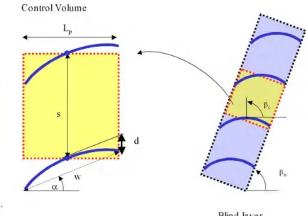
The thermal penetration length model stems from the fact that if natural convection is occurring in a gas space bounded by porous layers, the convective effect may penetrate a porous layer up to a certain length (or depth). The cavity convective heat transfer is, therefore, a function of this penetration length. To further illustrate this concept, consider a porous layer (j) of thickness Lp, forming a gas cavity with another
adjacent layer (j+1). The layer (j) is initially at a uniform temperature Tj. If the adjacent layer (j+1) is
maintained at a different temperature Tj+1, a buoyancy-induced flow may occur in the cavity, and the
thermal convection effect may penetrate the medium of layer (j) up to a distance δ (see Figure 2). This convection effect may invalidate the use of correlations for cavity film coefficient based on the cavity thickness Lj, as previously mentioned. It is, therefore, postulated that the film coefficient of cavity (hcavity)
may be obtained using the existing correlations for a cavity with a thickness equal to Lj + δ. The thermal
penetration length (δ), which is solely due to convection, depends on the geometrical and thermal characteristics of the layer medium (j), and the temperature difference (Tj+1 - Tj). It should, however, be
independent of the cavity spacing Lj. In this regard, if the front surface of layer (j+1) is moved to touch the
back surface of layer j, then the penetration length δ will be proportional to the average thickness of the boundary layer of a vertical (or tilted) plate at temperature Tj+1 adjacent to the layer medium (j). The
thickness of the boundary layer, itself, is proportional to the Rayleigh number as follows (Bejan, 2004):
m H Ra C H = ⋅ − δ / (16)
where (C) and (m) are constants and H is a characteristic plate height, which are to be determined according to the flow and layer types.
For slat-type blind layers, the airflow is restricted in the cavity between slats. The characteristic plate height H is, therefore, equal to the slat spacing (H = s), and the Rayleigh number RaH is given by:
υ
⋅
α
−
⋅
β
⋅
=
+ 3 1T
H
T
g
Ra
H j j (17) where: g : gravitational coefficient (m/s2; ft/s2) α : thermal diffusivity of cavity gas (m2/s; ft2/s). β : thermal expansion coefficient of cavity gas (K-1
; F-1). υ : viscosity coefficient of cavity gas (m2
/s; ft2/s).
The exponent (m) in Equation (16) may take on the following values 1/4 for laminar flows, 1/3 for turbulent flows, or intermediate values for mixed laminar and turbulent flows (Bejan, 2004). Using experimental measurements (see the validation section below), the constant (C) for laminar flows was found to be: 56 . 0 / = = m H H Ra Nu C (18)
where NuH is the Nusselt number for flows over a vertical (tilted) plate.
Similarly, Equation (16) may be used for drapery layers, but with a characteristic plate height H set equal to the window height.
It should be noted that the penetration length δ should be used only when the minimum cavity spacing Lj is finite and non-zero so that convection can take place in the cavity between layers. If both layers
touch (Li = 0), or if convection is not present in the cavity between layers (say when RaLi << 1), or if
convection is not present in the cavity between slats (say when RaH << 1), δ should be set to zero. Further,
(δ ≤ Lp/2). For slat-type blind layers, the layer thickness (Lp) designates the horizontal projection of slat
length (not its width). For drapery layers, the layer thickness (Lp) is given as shown in Figure 4.
The thermal penetration length (δ) should be calculated for each porous layer of a fenestration system. For example, If both cavity layers (j and j+1) are porous, the cavity thickness used to calculate the film coefficient should be equal to δj + Lj + δj+1. Finally, although Equation (18) was validated for laminar
cavity flows, which mostly occur in fenestration systems, care should be exercised to apply the equation to turbulent, or transitional flows without further validation studies.
It should be added that the above model for the convective film coefficient of gas cavity has some common things with the Reduced Slat Length model (RSL) of Wright et al. (2008). The latter model yields the following: ) cos( 2 / 3 . 0 ⋅ ⋅ α = δRSL w (19)
By comparing Equation (19) with Equation (16), one finds that the RSL model is developed for a specific blind product under specific boundary conditions. The model does not, however, account for the slat spacing (s) and thermal conductivity, and cavity temperature differential, which are inherent in Equation (16).
Screen Flow Model for Wind-Driven Forced Convection
Forced convection in cavities may occur using mechanical ventilation with known velocities, or unknown wind-driven ventilation. For cavities with porous layers open to the exterior environment, the wind-induced air velocity in a cavity may be obtained using the flow attenuation coefficient of the porous layers between the exterior environment and the cavity under consideration. For screen type layers (such as screen shadings and drapery sheets), the air velocity in a cavity may be obtained as follows (Miguel, 1998):
0.9
0.04
for
valid
;
89
.
0
⋅
ϕ
1.25⋅
1≤
ϕ
≤
=
j− jv
v
(20)where vj is the air velocity in cavity (j) sharing a porous layer with the front cavity (j-1) whose air
velocity is vj-1. Equation (20) was experimentally developed for screen shadings, but may be used for other
shading devices in absence of any suitable information. If the wind-driven velocities are weak so that natural convection dominates, the ISO ventillated cavity model (Equation 15) should, therefore, be used to calculate the cavity air velocity.
Effective Thermal Properties of Shading Layers
Shading layers can be grouped in three generic types: perforated plain screens, slat-type blinds, and draperies (or pleated shadings). Each porous shading layer is characterized by its porosity, which is defined as the ratio of the void volume to the total volume of layer.
Screen Shadings
A screen-shading layer is characterized by its openness factor (ϕ) and the yarn (or fibre) density (κ). The openness factor is defined as the ratio of the void surface area to the total surface area of a screen, and the yarn density is defined as the ratio of the average width of a yarn section to the screen layer thickness. The openness factor is also equivalent to the screen porosity (ω). In general, the screen material (fabric) may transmit, reflect and absorb thermal radiation. Using the averaging theory of porous media, the effective thermal properties of a screen layer are given by the following relationship:
(
)
m as P P
P = 1−ϕ ⋅ +ϕ⋅ (21)
where P stands for any given thermal property such as conductivity (k), density (ρ), or the product of density and specific heat (ρ cp). The subscripts (s, m, a) denote the screen layer, screen material (fabric)
Slat-Type blinds
Figure 3 shows a slat-type blind layer at a tilted window position. The blind slats may be opaque or perforated (with openness factor ϕs). The slats may enclose an open air space, particularly when they are
fully open (slat angle α = 0). If the blind layer is subject to a temperature difference at its front and back environments, a cellular flow may develop in the air space between slats (Machin et al., 1998; Naylor and Lai, 2007). This cavity flow may increase the heat transfer through the blind layer. Further, the environment air may flow though the porous blind layer, but its effect on heat transfer may be neglected due low velocities and relatively high-pressure losses through the blind layer. To account for the effect of the slat cavity flow on heat transfer, the air cavity is assumed as a solid material with an equivalent thermal conductivity. Temperature gradients through a blind layer denote thus the average of the slat and enclosed air cavity temperatures. Using a representative control volume as shown in Figure 3, the effective thermal properties of a blind layer are calculated as follows:
(
)
sm eq b k k k = 1−ω ⋅ +ω⋅ (22)(
)
sm a b = −ω ⋅ρ +ω⋅ρ ρ 1 (23)( )
ρcp b =(
1−ω)
⋅( )
ρcp sm +ω⋅( )
ρcp a (24) where:kb : effective thermal conductivity of blind layer (W/m.K; Btu/h.ft.F)
keq : equivalent thermal conductivity of the air cavity between slats (W/m.K; Btu/h.ft.F)
ksm : thermal conductivity of slat material (W/m.K; Btu/h.ft.F)
ρsm : density of slat material (kg/m3; lb/ft3)
The porosity of a blind layer (ω) is equal to one minus the ratio of the slat material volume to the volume of a representative control volume as shown in Figure 3:
(
s)
p s s s t s L t L + ⋅ ϕ − − = ω 1 (1 ) (25) where:Ls : length of blind slats (m; ft);
Lp : projected width of blind layer, see Figure 3, (m; ft);
s : spacing of blind slats, see Figure 3, (m; ft); ts : thickness of blind slat (m; ft);
ts : thickness of blind slats (m; ft);
ϕs : openness factor of blind slats(-);
Equation (25) accounts for curved slats, and therefore their effect on the thermal bridging is accounted for in the effective thermal conductivity of blinds.
The equivalent thermal conductivity (keq) of the cavity between slats may be determined based on the
convection film coefficient of a rectangular cavity subject to temperature differential at its open boundary surfaces and adiabatic conditions at slat surfaces as follows:
w z w T T h keq = c( h− c, , c,βc)⋅ (26) where:
hc : film coefficient of between slats cavity (W/m2K; Btu/h.ft2.F).
Th : temperature of the hot open surface of between slats cavity (K; F).
Tc : temperature of the cold open surface of between slats cavity (K; F).
w : thickness of between slats cavity (equal to the slat width) (m; ft). zc : height of between slats cavity (m; ft).
βc : inclination angle of between slats cavity (radians).
The height and inclination angle of the between slats cavity are determined as follow:
α
⋅
=
s
cos
z
c (27)α
+
β
−
π
=
β
π
>
β
α
+
β
=
β
c w,
if
c/
2
;
otherwise
c w (28) where: s : spacing of slats (m; ft). α : tilt angle of slats (radians).
βw : inclination angle of window (radians).
Drapes
Drapes are similar to screen shadings, except that the drapery fabric may be folded or pleated along the window width, hence forming open vertical pockets of air. In addition to the characteristics of a screen layer as mentioned above, drapes are characterized by the fullness factor (Fr), which indicates the ratio of the drapery fabric width to the window width. Fullness factors of 1.5 and 2 are typical values. The enclosed air pocket cavity may affect the heat transfer through the drapery layer if the latter is subject to temperature differential at its boundary environments. Further, the environment air may flow though the drapery porous layer, but its effect on heat transfer may be neglected due low velocities. Similarly, to a blind layer, flow within the air pocket cavities may be accounted for by an equivalent thermal conductivity. Equation (26) may, thus, be used for a drapery layer. Approximating the drapery configuration as a sequence of one-sided open rectangular cavity (Kotey et al., 2009a; Farber et al., 1963), as shown in Figure 4, the cavity characteristics used to calculate the film coefficient in Equation (26) are: cavity height (zc)
and tilt angle (βc) are equal to the height and tilt angle of window, and the cavity thickness (w) is equal to
the thickness of the drapery layer (Lp) minus the thickness of the drapery material fabric. Note that, the air
pocket cavities are finite in the direction of the fenestration width, and, therefore, proper correlations to account for the effect of cavity width (s) should be used to compute the film coefficient in Equation (26).
MODEL EXPERIMENTAL VALIDATION
The above models are implemented in the research version of SkyVision (NRC, 2008), and validated using the available experimental measurement of Huang (2005) for the center of glass U-factor of windows.
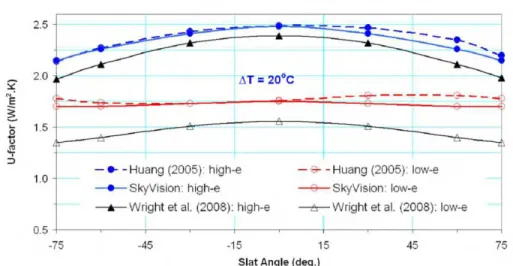
Huang (2005) and Huang et al. (2006) conducted laboratory measurements to compute the center of glass U-factor of a double glazed window with between pane Venetian blinds using the Guarded Heater Plate apparatus. The plate dimension were 635 mm (25 in) x 635 mm (25 in) (or 604 mm (23.78 in) x 604 mm (23.78 in) without the spacer section). Three sets of window cavity spacing were considered in the measurement: 17.78 mm (0.7 in), 25.4 mm (1 in), and 40 mm (1.575 in). The window was made up of two 3 mm (0.118 in) glass sheets with two high and low emissivity values (0.84 and 0.164 on the hot surface). The blinds were made of aluminium-alloy slats with the following characteristics: slat thickness = 0.2 mm (0.0078 in), slat width w = 14.79 mm (0.58 in), slat spacing s = 11.84 mm (0.466 in), slat curvature height d =1.5 mm (0.06 in), and slat emissivity of 0.792. To initiate heat flow through the window and blind system, the hot plate was maintained at a temperature of 30oC (86oF), and the cold plate took two temperature values of 20oC (68oF) and 10oC (50oF). The heat flux was measured at the hot plate at three locations: center and edge-end sections, each covering a surface area of 200 mm (7.87 in) x 200 mm (7.87 in). The center of glass U-factor was calculated based on the center heat flux measurement and assumed values for the interior and exterior film coefficients of 8 W/m2K (1.409 Btu/h.ft2.F) and 23 W/m2K (4.05 Btu/h.ft2.F), respectively.
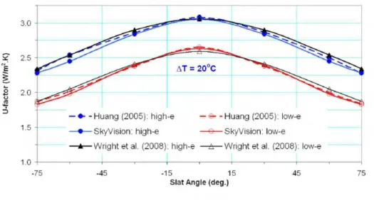
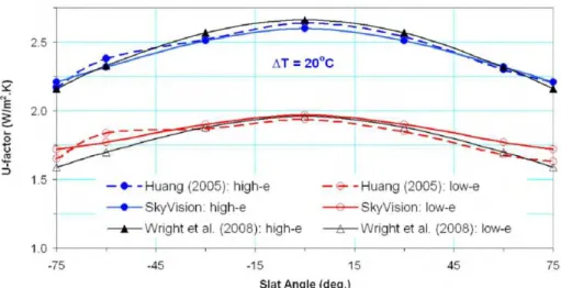
Figures 5 to 10 show a comparison between the measurement of Huang (2005) and the results from the current model for three window cavity spacing and two bath temperature differentials. The RSL model of Wright et al. (2008) is also shown in the figures. The predictions from the current model are in a very good
agreement with the measurement for both the high and low-emissivity windows. The maximum difference is less than 7%, which is observed for a window with a low-emissivity coating and small gap spacing when slats are almost closed (Figure 6). As previously stated, the RSL model is not suitable for large cavity spacing (e.g., 40 mm) as it under predicts the U-factor by 11% to 24%, particularly for windows with low-e coatings. Windows with such large cavity spacing are found in applications of double-skin facades.
CONCLUSION
This paper developed a general methodology to compute the thermal performance of fenestration systems incorporating shading devices, and elements imbedded in glazing layers for energy generation and conversion. The models assume each system layer as porous with calculated effective radiation and thermal properties. The effective thermal properties (such as conductivity, density and specific heat) of layers are calculated based on the geometrical and thermal characteristics of the layer medium and the effect of the convective heat transfer in the layer porous structure. Using the concept of the thermal penetration length, the effect of a shading layer on the convective heat transfer from its boundary surfaces to the adjacent gas spaces is also accounted for. A validation study was carried out, in which the U-factor of a double-glazed window with between-pane metallic Venetian blinds were compared with the laboratory measurement of Huang (2005). The comparison results showed that the model predictions were in very good agreement with the measurement, with a maximum difference less than 7%. It should be stressed that, despite the good comparison results, further validation work should be considered to cover other products and types of shading devices, window tilt configurations, and boundary conditions, particularly the ones that trigger turbulent flows in cavities between shades and glazing.
ACKNOWLEDGMENT
This work was supported by: the National Research Council of Canada; Natural Resources Canada; Canada Mortgage and Housing Corporation; Ontario Power Authority; Hydro Quebec, Gas Metro of Quebec; Pilkington USA; Prelco Inc.; Talius; and Lutron Electronics Corporation. The author is grateful for their contributions and continuous support to the project.
REFERENCES
Avedissian T., and Naylor D. 2007. Free convective heat transfer in an enclosure with an internal louvered blind. International Journal of Heat and Mass Transfer, 51, 283-293.
Avedissian T. 2006. A numerical study of free convective heat transfer in a double-glazed window with a between-pane Venetian blinds. MASc. Thesis, Ryerson University, Toronto, Ontario, Canada.
Bejan A. 2004. Convective heat transfer. Third edition. John Wiley & Sons, Inc. New Jersey.
Collins M.R, and Wright J.L. 2006. Calculating center-glass performance indices of windows with a diathermanous layer. ASHRAE Trans., 112:2, 1-8.
Collins M. 2004. Convective heat transfer coefficient from an internal window surface and adjacent sunlit Venetian blind. Energy and Building, 36, 309-318.
Collins M., Harrison S.J., Naylor D., and Oosthuizen P.H 2002a. Heat transfer from a isothermal vertical surface with adjacent heated horizontal louvers: numerical analysis. ASME Trans., 124, 1072-1077. Collins M., Harrison S.J., Naylor D., and Oosthuizen P.H. 2002b. Heat transfer from an isothermal vertical
surface with adjacent heated horizontal louvers: validation analysis. ASME Trans., 124, 1078-1087. Farber E.A, Smith W.A., Pennington C.W., and Reed J.C. 1963. Theoretical analysis of solar heat gain
through insulating glass with inside shading. ASHRAE journal, August, 79-90.
Garnet J.M. 1999. Thermal performance of windows with inter-pane Venetian blinds. MASc. Thesis, University of Waterloo, Waterloo, Ontario, Canada.
Huang N.Y.T. 2005. Thermal performance of double glazed windows with inter-pane Venetian blind. MASc. Thesis, University of Waterloo, Waterloo, Ontario, Canada.
Huang N.Y.T., Wright J.L., and Collins M.R. 2006. Thermal resistance of a window with an enclosed Venetian blind: Guarded Heated Plate measurements. ASHRAE Trans. 112:2, 13-21.
ISO. 2003. Standard 15099: Thermal performance of windows, doors and shading devices - detailed calculations. International Standard Organization; Geneva: Switzerland.
Kotey N.A., Wright J.L., and Collins M.R. 2009a. Determining off-normal solar optical properties of drapery fabrics. Submitted to the ASHRAE Trans.
Kotey N.A., Wright J.L., and Collins M.R. 2009b. Determining off-normal solar optical properties of roller blinds. Submitted to the ASHRAE Trans.
Kohl M. 2006. SHC Task 27: Performance of solar façade components: Performance, durability, and sustainability of advanced windows and solar components for building envelopes. Subtask A: Performance. International Energy Agency. Final Report.
LBNL. 2008. WINDOW 6.2: Windows and Daylighting Group, Lawrence Berkeley Laboratory, Berkeley, CA. URL: http://windows.lbl.gov/software/default.htm. Accessed in August 2008.
Loutzenhiser P. Manz H., and Maxwell G. 2007. Empirical validations of shading/daylighting/load interactions in building energy simulation tools. SHC Task 34 / ECBCS Annex 43 Project C. International Energy Agency. Draft for Final Report.
Machin A.D., Naylor D., Harrison S.J., and Oosthuizen P.H. 1998. Experimental study of free convection at an indoor glazing surface with a Venetian blind. HVAC&R Research, 4:2, 153-166.
Miguel A.F. 1998. Airflow through porous screens: from theory to practical considerations. Energy and Building, 28, 63-69.
Naylor D. and Collins M.R. 2005. Evaluation of an approximative method for predicting the U-value of a window with between-panes Venetian blind. Numerical Heat Transfer, Part A: Applications, 47, 233-250.
Naylor D. and Lai B.Y. 2007. Experimental study of natural convection in a window with between-panes Venetian blind. Experimental Heat Transfer, 20, 1-27.
Naylor D. Shahid H., Harrison S.J., and Oosthuizen P.H. 2006. A simplified method for modeling the effect of blinds on window thermal performance. International Journal of Energy Research, 30, 471-488.
NRC. 2008. SkyVision 1.2: National Research Council of Canada. URL:
http://irc.nrc-cnrc.gc.ca/ie/lighting/daylight/skyvision_e.html. Accessed in August 2008.
Phillips J., Naylor D., Oosthuizen P.H., and Harrison S.J. 2001. Numerical study of convective and radiative heat transfer from a window glazing with Venetian blind. International Journal of HVAC&R Research, 7:4, 383-402.
Shahid H., and Naylor D. 2005. Energy performance assessment of a window with horizontal Venetian blinds. Energy and Building, 37, 836-843.
Shahid H. 2003. A simplified technique for thermal analysis of a fenestration system with Venetian blinds. MASc. Thesis, Ryerson University, Toronto, Ontario, Canada.
Siegel R. and Howell J. 2002. Thermal radiation heat transfer. Fourth edition. Taylor & Francis. New York.
Safer N., Woloszyn M., and Roux J.J. 2005. Three-dimensional simulation with a CFD tool of the airflow phenomena in single floor double-skin façade equipped with a Venetian blind. Solar Energy, 79, 193-203.
WinDat. WIS Reference Manual (version 3.01). Window Thermatic Network. URL:
http://windat.ucd.ie/index.html. Accessed in August 2008.
Wright J.L., Collins M.R., Huang Y.T. 2008. Thermal Resistance of a window with an enclosed Venetian blind layer: a simplified model. ASHRAE Trans. 114:1. 1-12.
Wright J.L. 2008. Calculating the center-glass performance indices of glazing systems with shading devices. ASHRAE Summer meeting, Salt Lake City, June 2008.
Yahoda D.S., and Wright J.L. 2004a. Heat transfer analysis of a between-panes Venetian blind using effective long wave radiation properties. ASHRAE Trans. 110:1, 455-462.
Yahoda D.S., and Wright J.L. 2004b. Method for calculating the effective radiative properties of a Venetian blind layer. ASHRAE Trans. 110:1. 463-473.
Ye P., Harrison S.J., Oosthuizen P.H., and Naylor D. 1999. Convective heat transfer from a window with a Venetian blind: detailed modeling. ASHRAE Trans., 105:2, 1031-1037.
Zhang Z., Bejan A., and Lage J.L. 1991. Natural convection in a vertical enclosure with internal permeable screen. Journal of Heat Transfer, 113, 377-383.
Figure 1 Schematic description of a multi-layer fenestration system. Note that gas spaces are labelled differently than glazing layers
Figure 3 Schematic description of a slat-type blind layer
Figure 5 Comparison of U-factor values for a window cavity spacing = 17.78 mm (0.7 in) and bath temperature differential = 20oC (68 oF).
Figure 6 Comparison of U-factor values for a window cavity spacing = 17.78 mm (0.7 in) and bath temperature differential = 10oC (50 oF).
Figure 7 Comparison of U-factor values for a window cavity spacing = 25.4 mm (1 in) and bath temperature differential = 20oC (68 oF).
Figure 8 Comparison of U-factor values for a window cavity spacing = 25.4 mm (1 in) and bath temperature differential = 10oC (50 oF).
Figure 9 Comparison of U-factor values for a window cavity spacing = 40 mm (1.575 in) and bath temperature differential = 20oC (68 oF).
Figure 10 Comparison of U-factor values for a window cavity spacing = 40 mm (1.575 in) and bath temperature differential = 10oC (50 oF).