Appendix to "Distributional National Accounts: Methods and Estimates for the United States"

(1)

HAL Id: halshs-02794330

https://halshs.archives-ouvertes.fr/halshs-02794330

Preprint submitted on 1 Jul 2020

HAL is a multi-disciplinary open access archive for the deposit and dissemination of sci-entific research documents, whether they are pub-lished or not. The documents may come from teaching and research institutions in France or abroad, or from public or private research centers.

L’archive ouverte pluridisciplinaire HAL, est destinée au dépôt et à la diffusion de documents scientifiques de niveau recherche, publiés ou non, émanant des établissements d’enseignement et de recherche français ou étrangers, des laboratoires publics ou privés.

Appendix to ”Distributional National Accounts:

Methods and Estimates for the United States”

Thomas Piketty, Emmanuel Saez, Gabriel Zucman

To cite this version:

Thomas Piketty, Emmanuel Saez, Gabriel Zucman. Appendix to ”Distributional National Accounts: Methods and Estimates for the United States”. 2016. �halshs-02794330�

(2)

World Inequality Lab Working papers n°2016/4

Appendix to "Distributional National Accounts: Methods and Estimates for

the United States"

Thomas Piketty, Emmanuel Saez, Gabriel Zucman

Keywords : DINA; Distributional National Accounts; inequality; methodology;

income; wealth, national accounts; fiscal income; inequality measurement;

United States

(3)

Distributional National Accounts:

Methods and Estimates for the United States

Data Appendix

⇤

Thomas Piketty (Paris School of Economics)

Emmanuel Saez (UC Berkeley and NBER)

Gabriel Zucman (UC Berkeley and NBER)

December 15, 2016

Abstract

This Data Appendix supplements our paper “Distributional National Accounts: Methods and Estimates for the United States.” It provides complete details on the methodology, data, and programs.

⇤_{Thomas Piketty: piketty@psemail.eu; Emmanuel Saez: saez@econ.berkeley.edu; Gabriel Zucman:} zuc-man@berkeley.edu. We thank Tony Atkinson, Arthur Kennickell, Jean-Laurent Rosenthal, and numerous sem-inar and conference participants for helpful discussions and comments. Kaveh Danesh and Juliana Londono-Velez provided outstanding research assistance. We acknowledge financial support from the Center for Equitable Growth at UC Berkeley, the Institute for New Economic Thinking, the Laura and John Arnold foundation, NSF grant SES-1559014, and the Sandler foundation.

(4)

This data appendix supplements our paper “Distributional National Accounts: Methods and Estimates for the United States.” The appendix includes a large number of data files and computer codes, mostly in Excel and Stata formats. In section A, we describe the organization of these data files. In section B, we provide a number of supplementary methodological details on the imputations we make to create our U.S. distributional national accounts.

A

Organization of data files and computer code

Our data files and computer codes are organized into four parts. First are a number of raw data sources, which form the starting point of our project: macroeconomic aggregates from the national accounts, tax return micro-data, and survey micro-data. Second are theStata programs

that compute the distribution of U.S. national income starting from tax data, supplementing tax data using surveys, and making explicit assumptions for the categories of income which are not covered by tax or survey data. Third are our Distributional National Accounts micro-files, i.e., micro-files of synthetic observations representative of the U.S. population containing the national accounts income and wealth variables. Fourth are a number of Excel files with summary distributional results which were produced using the synthetic files. We describe each of these four components in turn and conclude this section by proving a list of all the files used in this research.

A.1 Raw data: macroeconomic aggregates, tax data, survey data

A.1.1 Macroeconomic aggregates

The first key data source used in this research is the national income and wealth accounts of the United States. All the macroeconomic series used in this research are gathered and presented in the Excel file Appendix Tables I (Macro). This file is built as follows.

First, Appendix Tables I (Macro)collects all the raw national income and wealth accounts published by U.S. statistical agencies. The National Income and Product Accounts (NIPA) of the United States, published by the Bureau of Economic Analysis (US Department of Commerce, Bureau of Economic Analysis, 2016), are collected in the sheet “nipa raw”. The Financial Accounts of the United States, published by the Federal Reserve Board, are collected in the sheet “ima raw”.1 _{Both the NIPAs and Financial Accounts are frequently updated; we regularly}

1_{The Financial Accounts of the United States, formerly known as the Flow of Funds, include data on the} flow of funds and levels of financial assets and liabilities by sector and financial instrument; full balance sheets, including net worth, for households and nonprofit organizations, nonfinancial corporate businesses, and nonfi-nancial noncorporate businesses; the Integrated Macroeconomic Accounts (an attempt at bringing together the

(7)

fetch updated series to reflect the latest data revisions and ensure full consistency with the current macroeconomic aggregates of the United States. The national accounts series currently included in Appendix Tables I (Macro) were downloaded in October 2016 from the websites of the Bureau of Economic Analysis and the Federal Reserve Board.2

Second, we have extended the U.S. income and wealth accounts backwards to 1913. The NIPAs start in 1929, while official Financial Accounts start in 1945. However, high-quality, well-documented historical accounts exist before the official series start. For income, we rely on the national income accounts of Kuznets (1941) for 1919–1929 and King (1930) for 1913–1919. For wealth, we combine balance sheets from Goldsmith, Brady, and Mendershausen (1956), Wol↵ (1989), and Kopczuk and Saez (2004) that are based on the same concepts and methods as the Financial Accounts.3 _{We adjust the historical series so as to ensure continuity with the} official statistics; all the adjustments are carefully documented in the sheets “DataIncome” and “DataWealth” of Appendix Tables I (Macro).

Third, we construct national income and wealth categories that are consistent with the 2008 System of National Accounts, the international standard for national accounting (United Nations, 2009). The U.S. macroeconomic statistics are generally broadly consistent with the SNA but di↵er in a number of ways. For instance, sectoral decompositions di↵er (U.S. accounts isolate a non-financial non-corporate business sector that does not exist in the SNA4_{); the} NIPAs use income concepts that do not exist in the SNA (such as personal income and net interest); and on the contrary the SNA includes decompositions of income that do no exist in the NIPAs (such as the decomposition of national income by sector5_{). McCulla, Moses and} Moulton (2015) provide a detailed comparison and reconciliation of the National Income and Product Accounts with the 2008 System of National Accounts. Because our ultimate goal is to be able to provide cross-country comparisons of inequality using similar methods and concepts, we have re-organized the U.S. national accounts so as to make them consistent with the SNA. This re-organization does not a↵ect the level or growth of national income and wealth, but makes comparing the components of national income and wealth across countries more straightforward.

NIPAs and the Financial Accounts in an accounting framework founded on the System of National Accounts); and additional supplemental details. They are published quarterly in US Board of Governors of the Federal Reserve System (2016).

2_{Downloading the raw national accounts series and integrating them into}_{Appendix Tables I (Macro)}_{is done} by the program scrap macro.do.

3_{The same historical income and wealth series were used by Saez and Zucman (2016).}

4_{this sector includes non-corporate businesses such as large partnerships that would be included in the} corporate sector in the SNA. As a result the share of the corporate sector in total value-added is low in the United States compared to other countries; see,e.g., Table I-A2 inAppendix Tables I (Macro).

(8)

The harmonized income and wealth categories we use—founded on the SNA—are described in Alvaredo et al. (2016).

The file Appendix Tables I (Macro) is organized as follows. Tables I-A1 to I-A10 provide series of U.S. national income and its components covering the 1913-2015 period. Tables I-B1 to I-B7 provides similar series for wealth, and Tables I-D1 to I-D8 for saving & investment. Tables I-S.A1 to I-S.A13, I-S.B1 to I-S.B3, and I-S.D1 to I-S.D4 provide supplementary decompositions of income, wealth, and saving & investment respectively.6

A.1.2 Tax data

The second key data source used in this research is micro tax data. Here we describe the raw tax data we used.

Public-use microfiles. Since 1962, there exists annual, high-quality public-use files (PUF) with samples of tax returns that have been created by the Statistics of Income (SOI) division of the Internal Revenue Service (IRS). The complete set of files and their documentation are maintained by Daniel Feenberg at theNBER.7 _{These files provide information for a large sample} of taxpayers, with detailed income categories. We have made these files comparable over time by constructing consistent income categories; this is primarily done by the program build small.do (see below). The most recent file available is for 2010. SOI is currently working on redesigning the PUFs. Once this redesign is completed, SOI plans to release the PUFs more timely and reduce the time lag (as had been the case in the past).

SOI individual income tax files. The PUF files are actually a subset of records and vari-ables coming out of the SOI individual tax return files that are created annually. These internal files are used for publishing official SOI statistics on individual incomes (US Department of Treasury, Internal Revenue Service, annual). This Statistics of Income: Individual Income Tax Returns provides detail on the sampling. The files are also used inside government tax agencies (US Treasury, Joint Committee on Taxation, and Congressional Budget Office) as a base for evaluating and scoring tax policies. The annual files are maintained since 1979.8 _{The most} recent file available is for 2014. Typically, the file for year t becomes available around July of

6_{In addition to the national account aggregates, we present totals for the flow of income reported to the IRS} (“fiscal income”) in Tables I-C1 to I-C6 (and I-S.C1 to I-S.C4) ofAppendix Tables I (Macro).

7_{There are no files for 1963 and 1965. A file for 1960 exists but with much fewer variables.}

8_{SOI files for 1960-1978 (except 1961, 1963, 1965) had also existed but have been lost. Only the public use} version remains.

(9)

year t + 2.

The files contain a much larger number of variables than the PUF. In particular, they include basic demographic information: age, gender, date of birth (and date of death). They also include a more detailed set of variables. In particular, they provide the breakdown of self-employment income across spouses. Starting in 1999, they can also be merged internally to the population-wide file of information tax returns to obtain the breakdown of wage earnings across spouses for married joint filers. Saez (2016) uses these internal files to create a set of basic tabulations of tax filers by age, gender, and earnings splits that allows to create synthetic versions of these demographic variables in the PUFs. Saez (2016) shows that the calculations using internal data vs. using the PUFs enhanced with these synthetic variables delivers very close results. The results published in this paper are created using the superior internal data whenever possible. In order to have the same set of programs working both externally on the PUF and internally on the SOI files, we have extracted and renames the variables in the SOI files using the variables names from the PUFs maintained at NBER and keeping a few extra variables such as gender, age, and earnings split within married couples that are needed in some of our series (these variables are added synthetically in the external PUFs in our programs).

Pre-’62 tax data. For the pre-1962 period, no micro-files are available so we rely instead on the Piketty and Saez (2003, updated to 2015) series of top income shares, which were con-structed from annual tabulations of income and its composition by size of income (US Treasury Department, Internal Revenue Service, annual since 1916). We made minor adjustments to the Piketty-Saez estimates to fix an inconsistency in the composition (but not in the level) of top incomes early in the twentieth century. Between 1927 and 1936, the composition of income in the top 10% and top 5% as estimated by Piketty and Saez (2003) is somestimes inconsistent in the sense that dividends, interest, rents and royalties earned by the top 10% and top 5% can exceed total taxable dividends, interest, rents and royalties.9 _{In order to address this issue, we} assume that no group of tax units above the 90th percentile can earn more than 95% of any income category; this condition is imposed in the the program pre62.do (described below) that

9_{This is mainly due to the following issue. Piketty and Saez (2003) add returns to account for the fact that} there are missing filers, as the exemption threshold for married couples is much higher than for singles. The added returns are added bracket by bracket ($1,000-$2,000, $2,000-$3,000, $3,000-$4,000, $4,000-$5,000) using extrapolation based on the ratio between the number of single men with no dependents and the number of married joint filers from other years. The problem is that composition tables for 1927-1936 do not break down brackets below $5,000. Piketty and Saez (2003) assumed that the added returns have the same income composition as all returns below $5,000, which is a problem because the composition of income changes significantly below $5,000. To account for that problem, they shaved o↵ a few points of dividend share in the composition tables from 1923-1937 for P90-95 and P95-99. They did, however, very little correction to rents/royalties and interest.

(10)

distributes national income and wealth before 1962.

A.1.3 Survey data

The third key ingredient of our distributional national accounts is survey data. We use two surveys: the Survey of Consumer Finances (SCF) and the Current Population Survey (CPS).

SCF. The Survey of Consumer Finances is available on a triennial basis from 1989 to 2013. It is a high quality survey that over-samples wealthy individuals. The Federal Reserve Board disseminates two sets of SCF files: summary extract public data (containing a number of key summary variables such as net wealth, expressed in inflation-adjusted dollars) and the full public data set (with the raw data in current dollars). We use both the summary extract and full public files. We rely on the SCF to impute forms of wealth (and therefore economic capital income) that cannot be captured by capitalizing income tax returns, see program use uscf.do described below.

CPS. We use the CPS March Supplement data, which are available since 1962 through the

NBER. We use the Stata programs available on the NBER website to convert the raw data files into Stata. For March 2014, we use the traditional CPS file rather than the re-designed survey. Complete documentation is available on the website of the Center for Economic and Policy research (CEPR). The CPS data are used to create a sample of non-filers (following the methodology developed by the Tax Policy Center for its tax simulator) and to impute a number of benefits that are not reported in tax data.

A.2 Programs creating US distributional national accounts

Here we describe the organization of the Stata programs we use in this research. The mas-ter program is runusdina.do; this program defines the paths and calls all the other programs described below. The programs are designed to run both externally using solely public use sources and internally within IRS using internal data. The external programs also use a series of additional basic tabulations based on internal data that are gathered in Saez (2016).

A.2.1 Programs using survey data

We start by constructing homogeneous SCF and CPS datasets, i.e., datasets that contain the same variables over time, and use them to compute the distributions of the income and wealth components that cannot be captured by tax data.

(11)

Program use scf.do. We use the SCF to estimate the distribution of housing wealth for non-itemizing tax units, mortgage debt for non-itemers, currency assets, and other debts. The program use scf.do (i) constructs SCF datasets with the relevant income and wealth variables using consistent definitions over time and (ii) estimates the distributions of housing, mortgage debt, non-mortgage debt, and currency assets.

Program use cps.do We use the CPS to estimate the distribution of a number of benefits that cannot (or only imperfectly) be observed in tax data: employee fringe health and pension benefits; Social Security benefits, Supplemental Security income, food stamps/SNAP, Veterans’ benefits, AFDC/TANF, and Medicaid. The programuse cps.do (i) constructs CPS datasets with the relevant income variables using consistent definitions over time and (ii) estimates the distribution of the above benefits. We also use the CPS to estimate how wage income is split among spouses in married couples for the years when we do not have information on this income split from tax data. See Section B.2 below.

A.2.2 Programs building tax data

Next, we construct homogeneous tax dataset, i.e., dataset that contain the same tax variables over time.

Program build small.do This program constructs annual datasets of income tax returns micro-data using the public-use micro-files (PUF). It starts from the public-use tax files dissem-inated through the NBER and constructs consistent income variables over time.

Program aggrecord.do This program adds a synthetic record to the homogeneous PUF files constructed by build small.do. The synthetic record insures that the total income in the PUF matches the total income reported to the IRS, component by component. Starting in 1996, the PUF have excluded extreme records from their sampling. From 1996 to 2008, the number of excluded records was small (between 13 and 191 in these years, as reported in the official PUF documentation), but large enough in income size to create significant discrepancies at the very top. Starting in 2009, the PUF excludes a larger number of extreme records (slightly over 1000) from its sampling but it aggregates all the excluded records into an aggregate record. We add a synthetic record to each PUF file over the 1996-2008 period; see Saez (2016) for more details.

(12)

Programs build xdata.do and build xfile.do. These programs are run on internal SOI tax files. They extract from the SOI files the variables available in the PUF and rename then following the PUF variables names used at NBER. They also merge in additional wage earnings split data from the population wide databank since 1999. These programs generate datasets that have the same structure as the PUFs but with additional variables such as demographic and earnings split information. The same program build small.do can also be run on these datasets.

A.2.3 Programs enriching public-use tax data

Next, we enrich the public-use micro-tax files by splitting income between married spouses, adding coarse demographic characteristics, and adding synthetic records for the income of non-filers.

Programs sharefbuild.do and addsharef. These programs split income between spouses in married couples. They use tabulations on earnings split from internal data from Saez (2016) and CPS data to estimate how the share of total income earned by the secondary earner varies with income (see Section B.2 below) and impute the earning split in the homogeneous PUF files constructed by build small.do.

Program impute.do This program imputes age and gender information in the post-1979 homogeneous PUF files constructed by build small.do using tabulations of internal SOI tax files presented in Saez (2016). It also imputes gender of single filers over the period 1962-1978.

Program nonfilerappend.do This program adds records representing non-filing households in the homogeneous PUF files constructed by build small.do. Non-filers are created using CPS data but adjusted to match statistics of non-filers for the period 1999-2014 presented in Saez (2016). See Section B.1 below for more details on the imputation of non-filers.

A.2.4 Programs creating DINA micro-files

Next, we combine the enriched micro tax data with survey data and national accounts data to create our distributional national accounts micro-files.

Program build usdina.do This program creates one distributional national accounts micro-file per year since 1962 (except in 1963 and 1965 when there are no publicly available samples of individual income tax returns). It uses the enriched PUF files constructed above, and from there

(13)

creates wealth variables matching Financial Accounts totals and income variables matching National Income and Product accounts totals. To do so, it calls the file parameters.csv that contains the national accounts totals constructed inAppendix Tables I (Macro). It splits income between spouses and imputes forms of income that are not captured by the tax data using the CPS and SCF distributions constructed in use cps.do and use scf.do

Program pre62.do This program construct top income and wealth shares matching national accounts macroeconomic totals for the period 1913 to 1961, when no micro tax data are available. It starts from the Piketty and Saez (2003, updated to 2015) series of top income shares, which were constructed from annual tabulations of income and its composition by size of income (US Treasury Department, Internal Revenue Service, annual since 1916).10 _{It then constructs factor} income, pre-tax income and post-tax income matching national income, making adjustments in 1962 to ensure consistency with post-1962 estimates obtained from micro-data. While our post-1962 distributional national accounts micro-file contain the full distribution (including for the bottom groups) of a wide range of national accounts variables, before 1962 we only focus on top groups (top 10% and above) and on a selected set of core national account variables. This selected set includes pre-tax income, post-tax income, wealth, taxes paid, transfers, and their components.

A.2.5 Programs producing statistics and exporting

Program outsheet dina.do This program computes a large set of summary distributional statistics using the 1962-onward annual distributional national accounts micro-files constructed by build usdina.do. These statistics are computed both on the internal data and on the external data. Saez (2016) compares the internal vs. external series. All series are gathered in the companion excel file of Saez (2016). In this paper, we use the internal series whenever they are available as they are based on more comprehensive data requiring fewer imputations.

Program graph dina.do This program combines the post-1962 summary distributional statis-tics created by build usdina.do with the pre-1962 top shares constructed by pre62.do to assemble homogeneous, long-run series of income and wealth share series and their components matching macro totals. It also export results to the Excel file Appendix Tables II (Distributions).

10_{All the issues since 1916 have been digitized by the Statistics of Income division of the IRS and posted online} at https://www.irs.gov/uac/soi-tax-stats-archivemaking this very rich and valuable data source easily accessible.

(14)

Programs taxrates.do, export dina.do and export-to-excel.do These programs make ad-ditional exports of the results.

A.3 Micro-files of U.S. distributional national accounts

A.3.1 External-use DINA files

The main output of this research in a set of annual micro-files representative of the U.S. economy, where each line is a synthetic individual created by combining tax, survey, and national account data, and each column is a variable of the national accounts. There is one file per year since 1962 (except in 1963 and 1965 when there are no publicly available samples of individual income tax returns). TheseDistributional National Accounts micro-filesare available online and structured as follows. The files are at the adult individual (aged 20 and above) level, so the sum of weights (variable dweght) adds up to the adult population, 226 million in 2010. The variable “id” identifies tax units, which makes it possible to compute statistics at the tax-unit level rather than adult level. The files also include socio-demographic information: age (restricted to three age categories, 20 to 44 years old, 45 to 64, and above 65), gender, marital status, and number of dependent children.

A.3.2 Codebook

Our Distributional National Accounts micro-filescontains the following 140 variables each year: 1. Socio-demographic characteristics

• id: Tax unit ID

• dweght: Population weight ⇥ 100,000

• dweghttaxu: Population weight to recover the Piketty-Saez total tax units

• female: Dummy for being female (PUF year 1969, 1974 and non-MFJ only, 2009 for all)

• ageprim: Imputed age of primary filer (husband if married)

• agesec: Imputed age of wife in married filers

• age: Imputed age

• oldexm: Dummy for primary filer being 65+

(15)

• old: Aged 65+

• oldmar: Interaction of married and old

• married: Dummy for being married joint return (filing status) • second: Dummy for being secondary earner

• xkidspop: Number of children (imputed to match population total ¡20)

• filer: Tax filer dummy 2. Core income and wealth series

• fiinc: Fiscal income (incl. capital gains) = fiwag + fibus + firen + fiint + fidiv + fikgi • fninc: Fiscal income (excl. capital gains) = fiwag + fibus + firen + fiint + fidiv

• fainc: Personal factor income = flinc + fkinc

• flinc: Personal factor labor income = flemp + flmil + flprl

• fkinc: Personal factor capital income = fkhou + fkequ + fkfix + fkbus + fkpen + fkdeb • ptinc: Personal pre-tax income = plinc + pkinc

• plinc: Personal pre-tax labor income = flinc + plcon + plbel

• pkinc: Personal pre-tax capital income = fkinc + pkpen + pkbek • diinc: Extended disposable income = dicsh + inkindinc + colexp

• princ: Factor national income (matching national income) = fainc + govin + npinc • peinc: Pre-tax national income (matching national income) = ptinc + govin + npinc +

prisupen + invpen

• poinc: Post-tax national income (matching national income) = diinc + govin + npinc + prisupenprivate + invpen + prisupgov

• hweal: Net personal wealth = hwequ + hwfix + hwhou + hwbus + hwpen + hwdeb 3. Detailed income and wealth series

(16)

• fibus: Fiscal income, business income

• firen: Fiscal income, rents

• fiint: Fiscal income, interest

• fidiv: Fiscal income, dividends

• fikgi: Fiscal income, capital gains

• fnps: Fiscal income (excl. KG), flat income for non-filers, matching PS shares

• peninc: total taxable pension income (=DB+DC+IRA withdrawals, but not Social Se-curity)

• schcinc: schedule net income

• scorinc: S corp net income

• partinc: partnership net income

• rentinc: net rental income from Schedule E = rentincp-rentincl

• estinc: estate and trust net income

• rylinc: royalties net income

• othinc: other income in AGI

• flemp: Compensation of employees

• flmil: Labor share of net mixed income

• flprl: Sales and excise taxes falling on labor (prop. to Y*(1-s))

• fkhou: Housing asset income

• fkequ: Equity asset income

• fkfix: Interest income

• fkbus: Business asset income

(17)

• fkdeb: Interest payments

• plcon: (Minus) social contributions (pensions + DI + UI, employers + employees + self-e

• plbel: Labor share of social insurance income (pensions + DI + UI)

• pkpen: (Minus) Investment income payable to pension funds (DB + DC + IRA, but excluding

• pkbek: Capital share of social insurance income (pensions + DI + UI)

• hwequ: Equity assets (div+KG capitalized)

• hwfix: Currency, deposits, bonds and loans of households

• hwhou: Housing assets

• hwbus: Business assets

• hwpen: Pension and life-insurance assets

• hwdeb: Liabilities of households

• flwag: Taxable wages of filers + non-filers

• flsup: Supplements to taxable wages

• waghealth: Health insurance contributions

• wagpen: Pension contributions (employer + employee)

• fkhoumain: Main housing asset income

• fkhourent: Rental housing asset income

• fkmor: Mortgage interest payments

• fknmo: Non-mortgage interest payments

• fkprk: Sales and excise taxes falling on capital (prop. to Y*(1-s))

• proprestax: Residential property tax (prop. to housing assets)

(18)

• rental: Tenant-occupied housing wealth, net of mortgage debt

• rentalhome: Gross tenant-occupied housing

• rentalmort: Mortgages on tenant-occupied houses

• ownerhome: Gross owner-occupied housing wealth

• ownermort: Mortgages on owner-occupied houses

• housing: Housing wealth, net of mortgage debt

• partw: Partnership wealth

• soleprop: Sole proprietorship wealth

• scorw: S-corporations equities

• equity: Equity assets (only div. capitalized)

• taxbond: Taxable fixed-income claims

• muni: Tax-exempt municipal bonds

• currency: Currency and non-interest bearing deposits

• nonmort: Non-mortgage debt

• hwealnokg: Net personal wealth (KG not capitalized)

• hwfin: Financial assets of households

• hwnfa: Non-financial assets of households

• plpco: (Minus) pension contributions (employer + employee + self-employed, SS + non-SS)

• ploco: (Minus) DI and UI contributions (employer + employee + self-employed)

• plpbe: Pension benefits (SS + non-SS)

• plobe: UI and DI benefits

(19)

• plpbl: Labor share of pension benefits

• plnin: Personal pre-tax labor income (narrow definition: pensions only)

• pkpbk: Capital share of pension benefits

• pknin: Personal pre-tax capital income (narrow definition: pensions only)

• ptnin: Personal pre-tax income (narrow definition: pensions only)

• dicsh: Disposable cash income

• inkindinc: Social transfers in kind

• colexp: Collective consumption expenditure

• govin: (Minus) Net property income paid by gov. (allocted 50% prop. to taxes, 50% to be

• npinc: Net primary income of non-profit institutions (prop. to disposable income)

• prisupen: Primary surplus (= contrib - distrib) of pension system

• invpen: Investment income payable to pension funds (DB + DC + IRA, but excluding life in

• prisupenprivate: Primary surplus (= contrib - distrib) of private pension system (al-locted prop.

• prisupgov: Government primary surplus (= taxes - benefits) (allocted 50% prop. to taxes, 50

• educ: Education collective consumption expenditure

• colexp2: Collective consumption exp. (with lump sum educ.)

• poinc2:

• tax: Total taxes and social contributions paid

• ditax: Current personal taxes on income and wealth

(20)

• ditas: State personal income tax

• salestax: Sales and excise taxes (prop. to Y*(1-s))

• corptax: Corporate tax (prop. to wealth excl. housing)

• estatetax: Estate tax

• govcontrib: Total contributions for government social insurance

• ssuicontrib: Contributions for government social insurance: pensions, UI, DI

• othercontrib: Contributions for government social insurance other than pension, UI, DI

• ssinc oa: Social Security income (old age)

• ssinc di: Social Security income (disability)

• uiinc: Unemployment insurance benefits

• ben: Total benefits (cash + kind + coll, excl. pensions, UI, DI)

• dicab: Social assitance benefits in cash

• dicred: Refundable tax credits

• difoo: Food stamps (SNAP)

• disup: Supplemental security income

• divet: Veteran benefits

• diwco: Workers’ compensation benefits

• dicao: Other social assistance benefits in cash

• tanfinc: TANF / AFDC benefits

• othben: Other cash benefits (State and local benefits similar to SNAP, etc.)

• medicare: Medicare = capitation for 65+ individuals

• medicaid: Amount of medicaid benefits received by tax unit

(21)

• pell: Pell grants received

• vethealth: Veteran in-kind health benefits

A.3.3 Internal-use DINA files

We have constructed similar distributional national accounts micro-files but starting from the internal use SOI files of individual income tax returns rather than the PUF tax files disseminated through the NBER. The internal-use files go from 1979 to 2014 and they contain exact age and gender information, exact self-employment earnings split, and exact wage earnings split since 1999. Before 1979, there are no internal files so external and internal computations are identical before 1979. The same set of programs builds both the external and internal dina files (and outputs the same statistical series). We use adjustments specific to external vs. internal data embedded in the programs with the use of a global macro data (equal to 0 for external and equal to 1 for internal).

A.4 Results: Distributional summary statistics

A.4.1 Main distributional results

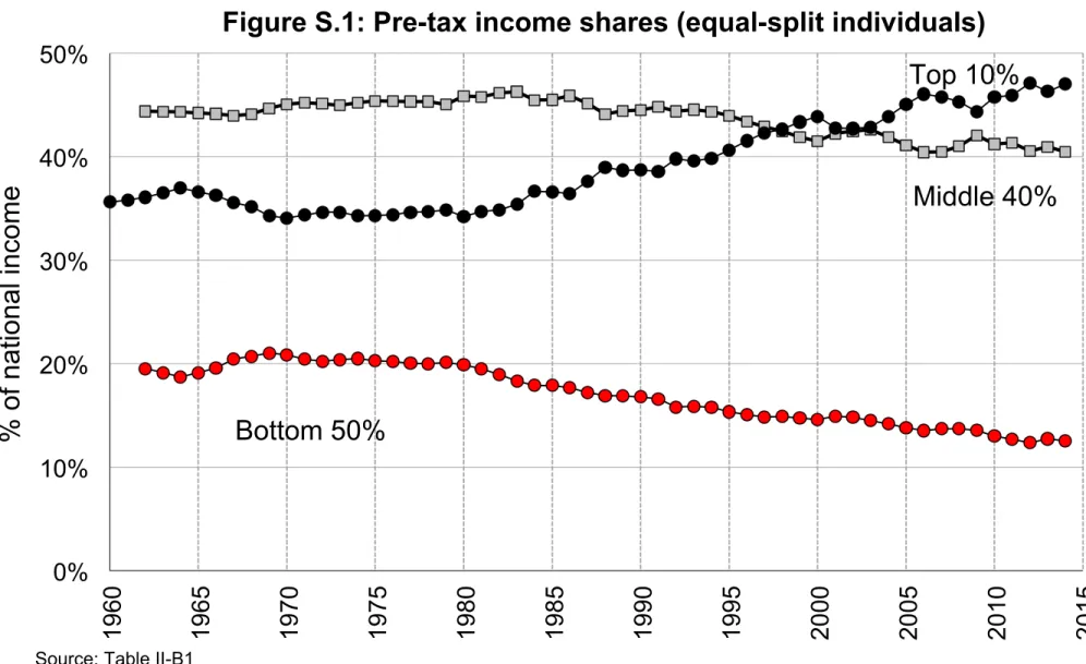
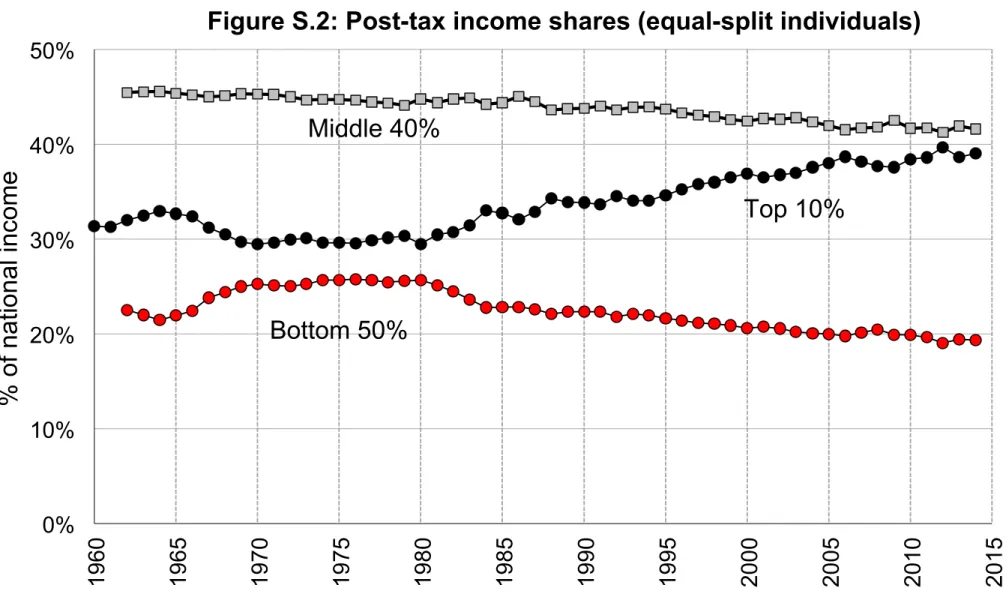
The main distributional results are presented in ourworking paper (Piketty, Saez and Zucman 2016) and the accompanying Excel file of Main Tables and Figures. This file includes the 13 Figures (with 2 panels each) and 2 tables included in the working paper, as well as a limited set of supplementary figures and tables (numbered FS.1, FS.2, TS.1, TS.2, etc.), which are also printed at the end of this appendix document.

A.4.2 Detailed distributional results

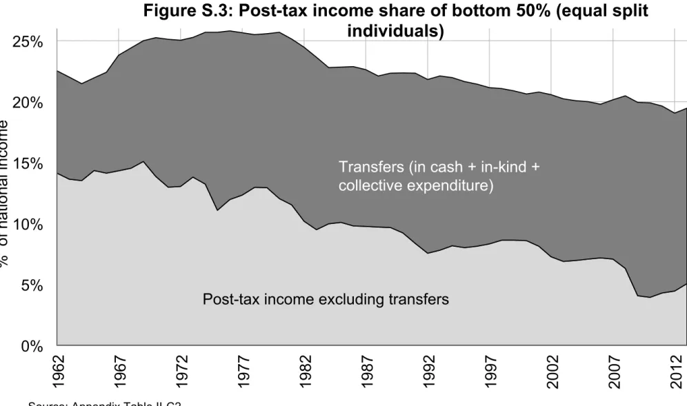
In addition to the main distributional results gathered in Main Tables and Figures, we present detailed appendix distributional results in the Excel file Appendix Tables II (Distributions). This file shows the distribution of factor income (Tables II-A1 to II-A14), pre-tax income (Tables B1 to B15), post-tax income (Tables C1 to C13), fiscal income (Tables D1 to II-D13), and wealth (Tables II-E1 to II-E13) with detailed decompositions. In addition, Tables II-F1 to II-F3 provide series on the gender labor income gap, average age by pre-tax income group, and the age-profile profile, and Tables II-G1 to II-G4 provide series on the distribution of taxes and benefits, with detailed decompositions.

(22)

A.5 List of online files

• Working paper: Text of the main paper, November 2016.

• Main Tables and Figures: Excel file with all the tables and figures included in the working paper and a small set of supplementary tables and figures.

• Appendix Tables I (Macro): Excel file with all the macroeconomic series used in this research (national income accounts, Financial Accounts, and historical national account series).

• Appendix Tables II (Distributions): Excel file with detailed distributional summary statis-tics.

• Distributional National Accounts micro-files: Stata micro-files of synthetic observations representative of the U.S., with detailed income and wealth components matching national accounts totals.

• Stata programs: Complete set of programs used to compute our distributional national accounts microfiles by combining tax, survey, and national accounts data.

• Data Appendix: Text of the Data Appendix, October 2016.

• Supplementary information on internal SOI computations: See “Improving the Individual Tax Return Public Use Files for Tax and Distributional Analysis” (Saez, 2016)

B

Supplementary information on imputations methods

All the details on the imputations methods we use are provided in the online computer code described above. Here we simply provide additional information on a number of issues.

B.1 Imputation of non-filers

About 10-15% of adults aged 20 and above do not file tax returns. To supplement tax data, we start by adding synthetic observations representing non-filing tax units using the Current Population Survey (CPS). We identify non-filers in the CPS based on their taxable income

(23)

following the methodology developed by the Tax Policy Center for their tax simulator.11 _We proceed in three steps.

First, we create tax units in the CPS data, then we apply filing thresholds to the tax units. As tax units with children are eligible for refundable credits, we assume that all tax units with children file tax returns whenever they have positive labor income. All tax units that fall below the filing thresholds are considered to be non-filers. Second, we re-weight these observations such that the total number of adults in our final dataset matches the total number of adults living in the United States, for both the working age population (aged 20-65) and the elderly (above age 65). The weights are fairly close to one in general. Third, we have used the detailed tabulations on statistics for non-filers from IRS data for 1999-2014 presented in Saez (2016) to adjust the CPS based non-filers. Social security benefits, the major income category for non-filers is very close and does not need adjustment. However, there are more wage earners and more wage income per wage earner in the IRS non-filers statistics (perhaps due to the facts that very small wage earners may report zero wage income in CPS and a fraction of individuals with wages may fail to file income tax returns). Over the period 1999-2014, there about twice as many wage earners in the IRS non-filer sample than in our CPS built sample of non-filers, and conditional on being a wage earner, they earn about twice as much as in the IRS non-filer sample than in the CPS. Hence, when building the CPS sample (and before adjusting weights for age), we simply re-weight wage earners in the CPS by a factor 2 and we uniformly increase their wages by a factor 2. With these adjustments, the CPS based sample of non-filers has about as many wage earners and the same aggregate wage amount as the IRS non-filer sample for the period 1999-2014. We apply the same adjustment to wages retro-actively over the full period 1962-2014.12

11_{Tax simulators typically rely on tax return data. However, for some tax simulations (such as reducing} exemptions or deductions), it is important to capture the population of non-filers as some current non-filers might become taxpayers. Hence, the Tax Policy Center developed a method to model non-filers using CPS data. Their methodology is presented in detail in Rohaly, Carasso, and Adeel Saleem (2015). We thank the Tax Policy Center for sharing their programs with us allowing us to build on their work.

12_{In the future, it might be possible to construct a file of non-filers using exclusively tax data as done in Saez} (2016). We have not followed this route because non-filers can be obtained from tax data only for the period 1999-2014. Furthermore, there is no simple route to determine the marital status and link spouses together in the non-filer IRS data. The spousal link is important as we split income equally across spouses in our benchmark series. A fairly large numbers of non-filers are retirees with only Social Security Income, a significant fraction of whom are married.

(24)

B.2 Imputation of income split among spouses

Because the US income tax is family based, one needs to supplement income tax returns by other data sources to estimate individual income. The CPS contains information on individual income but not in top groups because of top coding. Individual income is available from W2 tax forms, but only since 1999 and a few years isolated years before 1999 (namely 1969, 1974, and 1982-6). We therefore proceed as follows.

First, we always split capital income and wealth 50/50 because of the lack of data on property regimes. Next, we estimate individual wage income by combining CPS and tax data. We use the CPS to estimate the wage split among couples in the bottom 95% of the wage income distribution among married couples with positive wage income. We use tax data to estimate the wage split in the top 5%. More precisely, for 1969 and 1974, wages from W2 tax forms are included in the public-use micro-files of tax returns. Between 1982 and 1986, secondary earners had a tax credit and therefore wage split information is also included in the PUF. Since 1999, we rely on tabulations of share of female wages in total family wages by fractiles of family wage income (among married joint filers with positive wage income) computed in the internal-use SOI samples files (presented in Saez, 2016).13 _{For the years with no direct information, we linearly} interpolate the wage split using the closest years with available data. We have checked that this imputation method delivers results that are close to the results obtained for years when we have exact wage split (1969, 1974, and 1999-2014).

Regarding self-employment income, we assume that 70% of self-employment income is labor income and 30% is capital income. We split the capital portion 50/50 (just like other forms of capital income). We split the labor portion of self-employment income using tax based information on the split of self-employment income across spouses (this information is reported on tax returns individually for each spouse on the Schedule SEs). In external tax data, the self-employment individual earnings variables are capped (and start in 1984) but they are fully uncapped and start in 1979 in internal data. In internal computations, we use the exact split for 1979 on. In external computations, we use the exact split when the variables are not capped. When the variables are capped, we rely on tabulations of the share of self-employment income earned by the female spouse by fractiles to family self-employment income in married couples with positive self-employment income. These tabulations are presented in Saez (2016). Before 1979, we assume that the split of the labor portion of self-employment income is the same as in 1979. Last, we split benefits and pension income 50/50.

(25)

B.3 Imputations of wealth and income from survey data

B.3.1 General imputation method

Generally speaking, our strategy to impute income or wealth components seen in surveys but not in tax data is the following. Take an income or wealth component y, for instance Veterans’ benefits or non-mortgage debt. First, we use survey data to estimate the probability that a tax unit earns or owns y in each of the 40 following bins: decile of the taxable income distribution ⇥ marital status ⇥ primary earner above or below 65 years old. We then compute the average amount of y (conditional on earning/owning y) in each bin. Next, in the enriched tax data created by the program build small (see above), we randomly impute y in each bin of taxable income decile ⇥ marital status ⇥ above 65 using the probability distributions estimated in the surveys and assigning the bin-specific average amount of y to each recipient. We adjust the number of recipients and/or the average amount of y proportionally in each bin in order to match macroeconomic totals. For instance, we adjust the number of imputed Medicaid beneficiaries so as to match the true number of beneficiaries from administrative records; we adjust the average amount of imputed non-mortgage debt such that total non-mortgage debt adds up to the total recorded in the Financial Accounts.

For some types of income, we implement variants of this imputation method which can be either more sophisticated (e.g., using more detailed bins, such as for Medicaid benefits) or less sophisticated depending on data availability. In a number of important cases we have also checked the consistency between the distribution of our imputed income components and information available from other sources.

The advantage of our imputation method is that it is simple to implement and overcomes automatically issues of under reporting in the Current Population Survey that are well known (see Meyer, Mok, and Sullivan 2009, 2015 for detailed analyzes and discussion). Our method does not require developing a sophisticated and granular benefit calculator either.14 _Our im-putation is designed to respect the correlation of benefits recipiency with income, marital, and elderly status.

The drawback of our imputation method is that it fails to capture correlations in benefits recipiency across programs (for example, TANF recipients are automatically eligible for Medi-caid, etc.), or the fact that recipiency is often correlated with observable characteristics (such as age or presence of children in the household). Importantly, our methods should be seen as a

14_{The most extensive e↵ort to create a benefit simulator in the United States is the Transfer Income Model} (TRIM) of the Urban Institute. See Zedlewski and Giannarelli (2015) for a general presentation.

(26)

simple initial benchmark which will could be further refined and improved down the road.

B.3.2 Wealth imputations

We construct wealth by capitalizing income tax returns and accounting for the forms of wealth that do not generate taxable income, as in Saez and Zucman (2016). The only methodological di↵erence with Saez and Zucman (2016) is that we provide better imputations of housing wealth for non-itemizers, mortgage debt for non-itemizers, currency assets, and other debts. Namely, we compute the distribution of these assets in the SCF and randomly impute them to tax units following the method described in Section B.3.1 above; see program use scf.do.

B.3.3 Income imputations

Employee fringe benefits Pension contributions are only imperfectly captured in the CPS. The CPS provides information on who is covered by an employee pension plan, but does not provide data on the amounts contributed, which can be hard to know for respondents, in particular in the case of defined benefit plans. Therefore, we use the CPS to impute the probability to be covered by a pension plan by income decile⇥ marital status ⇥ above 65; within each bin we then assume that the pension contributions are proportional to wages winsorized at the 99th percentile. We winsorize because there are annual caps on defined contributions such as 401(k)s. Defined benefit plan tend to be proportional to wages (often with a cap). We have checked using IRS Statistics of Income tabulation of elective pension contributions and retirement plan indicators by brackets of wage income that this is a reasonable assumption.15

Health benefits are better captured in the CPS as there is information on the cost of health insurance plans. We therefore apply our standard imputation method described in Section B.3.1 above. Since 2012, health benefits have been reported on W2 forms. We have checked that the distribution of health benefits in the CPS and our imputed series is consistent with the high-quality information available in internal-use SOI sample tax files. In the future, it should be possible to use these data to do better imputations of employer based health insurance benefits.

Individualized transfers We use the CPS to estimate the distribution of the following indi-vidualized transfers: Social Security benefits, Supplemental Security income, food stamps/SNAP, Veterans’ benefits, AFDC/TANF, and Medicaid. We follow the imputation strategy described

15_These _statistics _are _available _online _for _years _2008-2010 _at _{https://www.irs.gov/uac/}

soi-tax-stats-individual-information-return-form-w2-statistics. In the future, it should be possible to use these data to do better imputations of pension contributions.

(27)

in Section B.3.1 above; that is, we compute the joint distribution of taxable income and Social Security benefits (resp. Supplement Security income, SNAP, etc.) by estimating the probability to receive Social Security in 40 income bins (decile of the taxable income distribution ⇥ marital status _{⇥ above or below 65 years old), and we then compute the average amounts of Social} Security benefits (resp. Supplement Security income, SNAP, etc.) in each bin conditional on receiving Social Security income (resp. Supplement Security income, SNAP, etc.). For Medi-caid, we use more detailed bins (8 income groups _{⇥ marital status ⇥ number of kids ⇥ number} of Medicaid recipients).

B.4 Imputation of taxes

Computing pre-tax income shares requires making tax incidence assumptions. As is well known in tax incidence theory, the burden of taxes is not necessarily borne by the economic agent who nominally pays them. Behavioral responses to taxes can a↵ect the relative prices of factors hereby shifting the tax burden on a given factor to other factors. Taxes, on top of being shifted, also generate deadweight burden (see Fullerton and Metcalf, 2002 for a survey of the economic literature). In this paper, we do not attempt to measure the complete e↵ects of taxes and transfers on economic behavior and ultimate money-metric welfare of each individual. There is a long tradition in federal government agencies to present distributional tables of the Federal tax burden which naturally require making tax incidence assumptions (see e.g., US Congressional Budget Office (CBO), 2016). We discuss how we depart from the official CBO tax incidence assumptions. In contrast to CBO statistics, we compute taxes not only at the federal level but also include all taxes at the State and Local level.16 _{We make the following simple assumptions} regarding tax incidence.

B.4.1 Individual income and payroll taxes

We assume that individual income taxes are paid by individual taxpayers with no further in-cidence. We also assume that payroll taxes are paid entirely by labor, regardless of whether they are nominally paid by employers or employees. Because we expect labor demand to be more elastic than labor supply, standard tax incidence theory predicts that payroll taxes should primarily fall on workers (see e.g. Hamermesh 1993). This has been the standard assumption in most analyzes of the distributional e↵ects of taxes and is the CBO assumption as well.

16_{In contrast to federal taxes, there are no systematic or official statistics on the tax incidence of state and} local taxes, owing to the decentralized nature of US governments, each local government having its specific tax system.

(28)

B.4.2 Corporate income tax

We assume that the corporate income tax falls on all capital except housing (net of mortgage debt). In practice, this means that equity owners bear only about 45% of corporate taxes, since equity wealth (including equities held through pension plans) is about 45% of all non-housing wealth today. The owners of fixed income claims (deposits, bonds, etc., including held through pension plans) bear about 40% of the corporate tax, and the owners of non-corporate business assets the remaining 15%; see Appendix Table I-S.A9. Because the e↵ective tax rate on U.S. corporate profits (i.e., the amount of corporate tax paid divided by the flow of corporate profits accruing to U.S. residents, either from domestic or foreign-owned corporations) has been around 25% in recent years, our assumptions imply that all equity owners pay around around 25% _{⇥ 45% = 11.25% in corporate taxes out of the corporate profits that accrue to them.} One implication is that in our distributional national accounts, by construction billionaires—for whom almost all wealth is equity and all income is corporate profits—cannot have an overall tax rate below 11.25%. This is true including for the owners of companies that in practice pay zero or very small amounts of corporate taxes.

Note that in the U.S. national accounts, the profits made by the Federal Reserve System are treated as corporate taxes received by the Federal government. These profits have been large since the financial crisis of 2008-09 and the subsequent expansion of the Fed’s balance sheet. They amounted to about $80 billion in 2013, almost 20% of all corporate income taxes received by U.S. governments, Federal and States. We have followed the U.S. national accounts convention of treating the Federal Reserve Systems’s profits as corporate tax revenue for the government, although it seems more meaningful to view these profits as dividends paid to the government rather than taxes. We may change our treatment of Fed’s profits in the future as we learn more about how other countries proceed.17

CBO assumes that corporate taxes fall 75% on capital and 25% on labor (CBO earlier assumed that corporate taxes fell 100% on capital).18 _{We think that the assumption of 100%} incidence on capital is a more reasonable benchmark as there is no compelling empirical evidence that corporate taxes depress wages in a large economy like the United States. If the corporate tax

17_{Zucman (2014) removed Fed’s profits for corporate tax revenue to compute e↵ective corporate tax rate on} U.S. corporate profits, which explains why he finds e↵ective corporate tax rates around 20% rather than the 25% implied by a naive computation that does not remove Fed’s profits.

18_{The Tax Policy Center (TPC) (an external non-governmental think-tank) assigns 80% of the corporate tax} burden on capital and 20% on labor. However, in practice, CBO and TPC do not assign corporate taxes on all forms of capital, but solely on capital income reported on individual tax returns, hereby excluding pension funds from the corporate tax burden.

(29)

is partly shifting on labor income, then the overall tax system would be slightly less progressive that what we obtain here. It is fairly easy to modify our programs to change our assumption on corporate tax incidence.

In contrast to CBO, we do not assume that the corporate tax falls on housing capital because we think the housing market vs. the corporate equity market are not sufficiently integrated as we discuss just below.

B.4.3 Property taxes

About 60% of property taxes are business property taxes; the remaining 40% correspond to residential property taxes. We assume that business property taxes are borne by all capital excluding housing, just like the corporate tax, and that residential property taxes are borne by the owners of housing assets. These assumptions are consistent with the following model that has two forms of capital: corporate assets vs. housing assets (in the spirit of Harberger, 1962). With an infinite elasticity of substitution between di↵erent forms of capital, the after-tax rate of return must be the same for all forms of capital assets. In such a model, any tax on a capital asset is e↵ectively shifted on all capital assets (this is the CBO assumption for corporate taxes). While the elasticity of substitution between di↵erent forms of financial assets is probably very high, there seems to be relatively little substitutability between housing and non-housing. Typically, many families own real estate as a place to live and own corporate assets through their pension funds without arbitraging between assets as in a standard frictionless asset pricing model. This motivates our assumption to treat housing and non-housing assets as two separate sectors, and within the non-housing sector to assume that taxes fall broadly on all forms of non-housing assets. In the housing sector, the incidence of the residential property tax then depends on how elastic housing supply and housing demand are. If the supply of housing is not elastic (e.g., it is impossible to build new housing units due to lack of land or excessive regulations) relatively to the demand of housing, then the incidence of the property tax falls on the owners of housing; if the supply of housing is very elastic (land is plentiful so that new housing can be built at a fixed marginal cost), then the incidence falls on tenants. There is evidence that in the short run, housing supply is not very elastic and therefore that housing subsidies benefit landlords and property taxes are paid by landlords. Fack (2006) finds that in France, one additional euro of housing benefit leads to an increase of 78 cents in the rent paid by new benefit claimants. There is more uncertainty regarding the long-run incidence of residential property taxes; in the long run, housing supply may become more elastic, shifting part or all of

(30)

the burden of residential property taxes to tenants. Using our micro-files, it is straightforward to assume that a fraction of residential property taxes is shifted to prices rather than borne by capital owners. We have tested the extreme scenario where housing supply is infinitely elastic and residential property taxes are entirely shifted to prices. Because the residential property tax is modest in the U.S. ($166 billion in 2015, only 3% of total tax revenue), this makes only a small di↵erence on our pre-tax income series.

B.4.4 Sales and excise taxes

We assume that excise and sales taxes are paid proportional to disposable income less savings.

B.5 Collective consumption expenditure

Computing post-tax income by adding back to individuals all forms of government spending requires making assumptions on who benefits from non-individualized government transfers, i.e., collective consumption expenditure for education, defense, etc.

B.5.1 Health spending

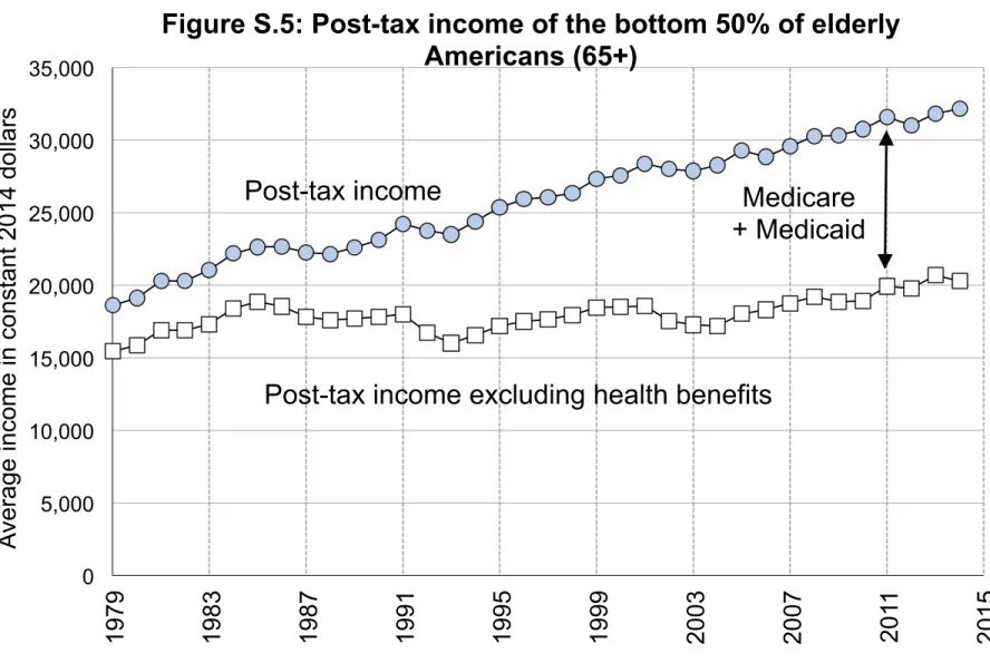
We assign Medicare and Medicaid benefits to beneficiaries on a lump sum basis; i.e., every Medicare-eligible adult gets the same benefit (about $10,000 today) and every Medicaid-eligible individual (adult or child) gets the same benefit (about $5,000 today). The benefits received by children are added to their parents’ income.

For comparability with countries where there is no information on the age profile of govern-ment health benefits (which is typically the case in single-payer systems where almost all health spending is paid for by the government), we also provide additional series where we assign all Medicare and Medicaid beneficiaries the same average transfer (equal to total Medicare plus Medicaid spending divided by the total number of beneficiaries). One drawback of this proce-dure is that the Medicare lump sum transfer is significantly higher than the Medicaid lump sum transfer (about twice higher in recent years) and has been growing faster. Disregarding this heterogeneity artificially inflates the post-tax income and income growth of Medicaid-eligible working-age Americans.

B.5.2 Education spending

In our benchmark series, we allocate public education spending proportional to disposable in-come as well. This can be justified from a lifetime perspective where everybody benefits from

(31)

education, and where higher earners attend better schools and for longer. We have also con-sidered a polar alternative where we consider the current parents’ perspective and attribute education spending as a fix lump sum per child. In married couples, we attribute each child 50/50 to each parent. Note that children going to college and supported by parents are typically claimed as children dependents so that our lump sum measure gives more to families supporting children through college. This slightly increases the level of bottom 50% post tax incomes but without a↵ecting the trend

B.6 Imputations to match national income

B.6.1 Income of non-profits

B.6.2 Government deficit and interest payments on debt

In general, a government deficit means either higher taxes, lower government transfers or both in the future. Taxes can be implicit, e.g., financial repression (lowers returns on assets; may also lower bankers’ wages). Transfer reduction: case of 19th century UK with arguably lower educational spending compared to counterfactual without Napoleonic war debts. Whether taxes or transfers adjust depends on regime (democracy vs. oligarchy), maybe the type of event generating the deficit (war vs. financial crisis; cyclical vs. structural), so no general rule on whether deficit should be seen as a↵ecting future taxes more or less than future transfers. So to allocate the deficit to the existing population, we reduce everybody’s transfers and increase everybody’s taxes proportionally and with equal weights on taxes and transfers.19

Interest income paid on government debt is included in individuals pre-tax income but is not part of national income (as it is a transfer from government to debt holders). Hence, in our pre-tax measure, we also deduct interest income paid by the government in proportion to taxes paid and benefits received (50/50) in the same way we treat government deficit.

19_{A more sophisticated possibility would be to allocate the deficit based on age}

⇥ taxes paid ⇥ transfers received (rather than taxes paid _{⇥ transfers received only). For instance, if government deficit is due to public} transfers to elderly being bigger than taxes, and if people have life-cycle saving motive only, then currently young people are those who will ultimately have to pay more taxes/receive less transfers_{! deficit could be seen} as reducing young people’s current transfers and increasing their current tax liabilities, leaving the disposable income of the elderly unchanged. Generational accounting is heavily influenced by this life-cycle saving view and so tends to see government deficit as a↵ecting young people disproportionately. But if people have dynastic preferences, then the deficit will trigger increased saving by current pensioners, reducing their income available for consumption; in that case it’s less clear that the deficit should only be allocated to young people.

(32)

B.6.3 Surplus of pension system

We o↵er two treatments for pensions. In our “factor income” series (Appendix Tables II-A1 to II-A14,), we treat pensions on a contribution basis. That is, we include all pension contributions and payroll taxes in our factor income flow, and we exclude all pension distributions from it. One problem with the concept of factor income is that it allocates little income to retirees who mostly live o↵ of pension distributions, and therefore it tends to overestimate inequality in aging societies (although one can always look at inequality within the working-age population). That is why we prefer to use “pre-tax income” as our benchmark concept for the distribution of income before government intervention. In our pre-tax income series (Appendix Tables II-B1 to II-B15), pensions are treated on a distribution basis. That is, compared to factor income, pre-tax income deducts contributions and adds back pension benefits.

In a given year there is usually an imbalance between pension contributions and distributions. In the United States, as shown by Appendix Table I-A7, pension contributions have been significantly larger than distributions over the last decades. Pension contributions include all Social Security contributions (the old-age portion of payroll taxes paid by employers, employees, and the self-employed, $683 billion in 2015), non-Social Security contributions paid out of labor income (payments made by employers and employees to defined contributions plans; payments made by employers to defined benefit plans; contributions made by workers to their individual retirement accounts out of pre-tax income—all of which add up to $921 billion in 2015), and the capital income earned by pension plans that is immediately reinvested in those plans ($1,316 billion in 2015). In total, pension contributions amounted to $2,920 billion in 2015; seeAppendix Table I-A7 and I-A.S10 for a detailed decomposition. By contrast, distributions amounted to $1,706 billion only.

The excess of pension contributions over distributions can be decomposed into three terms: the surplus of the pay-as-you-go public pension system (Social Security), the primary surplus of private pensions (the excess of private pension contributions excluding reinvested capital income over private pension distributions), and the capital income reinvested in private pension plans. As shown by Appendix Table I-A10, Social Security had a small surplus from 1984 to 2008, and has had a small deficit since 2009 (about $100 billion in 2015). The primary surplus of private pensions is roughly zero. So as a first approximation the primary surplus of the overall pension system (Social Security + private pensions) is close to zero, i.e., pension distributions are roughly equal to the sum of all contributions paid out labor income. Almost all the gap between total pension contributions and distributions comes from the large amount of capital

(33)

income reinvested in pension plans.

An economy with funded pensions naturally tends to have contributions greater than dis-tributions (see Alvaredo et al. 2016). To see this, consider an economy in steady-state growth (fixed demographic and productivity growth rates, with a stable age structure) with a total growth rate equal to g = n + h (the sum of demographic and productivity growth), and an average return to capital equal to r. With a pay-as-you-go pension system, contributions are equal to pensions (disregarding small accounting surpluses or deficits), so that personal pre-tax income is equal to personal factor income in aggregate. However with a funded pension system with total steady-state pension wealth equal to WP t = P · Yt (where Yt is personal factor income, growing at rate g; WP t is pension wealth, also growing at rate g; and P is the steady-state pension wealth-factor income ratio), one can immediately see that contributions (including accrued investment income) exceed pension distributions by g·WP t.20 So for instance if g =2% and steady-state pension wealth represents 300% of personal factor income, then in steady-state pretax income will be equal to 96% of personal factor income in a country with funded pensions (and 100% in a country with pay-as-you-go pensions). In the United States, as shown byAppendix Figure S.24, personal pre-tax income has fallen from 100% of personal factor income in the 1960s to 90% in the mid-1990s, and has slightly rebounded since then to 92.5% in 2015. This ratio is low because pension wealth is still accumulating and has not reached a steady state yet: pension wealth is 160% of national income is still rising; see Appendix Table I-B2). As we approach a steady-state, the ratio of personal pre-tax to personal factor income should rise above 95%.

Because we want to match national income in all our series—whether looking at factor income, pre-tax income, or post-tax income—we allocate to individuals the excess of pension contributions over distributions. This procedure ensures that our pre-tax income total is the same as our factor income total (and equal to national income), which makes comparing growth rates straightforward. We proceed as follows. First, we allocate the surplus of the Social Security pension system proportionally to taxes paid and benefits received, just like we do for the general government deficit. This assumes that Social Security is fungible with other government revenue and expenditure, i.e., that any deficit will eventually have to be addressed by raising taxes or cutting government transfers.21 _{Second, we allocate the (very small) primary} surplus of the private pensions system proportionally to wages. Last, we re-attribute the capital

20_{Denote by ct} _{contributions out of labor income and dt} _{distributions, we have WP t+1} _{= (1 + g)WP t} ₌ (1 + r)WP t+ ct dt so gWP t= rWP t+ ct dt, which is the excess of total contributions over distributions.

(34)

income reinvested on pension plans to the owners of pension wealth. If the pension system was in a steady-state, it would be preferable to reattribute this income to retirees only for pre-tax income (in contrast to factor income). But since the U.S. private pension system is still in accumulation, we choose instead to reattribute investment income to both pensioners and retirees in proportion to their share of pension wealth, so as to avoid artificially impoverishing working-age adults. In recent years, about 60% of pension wealth belongs to retirees and 40% to wage-earners.

B.7 Other

B.7.1 Unit of observation

Our unit of observation is the adult, i.e., we allocate total national income to all US residents aged over 20.22 _{This seems preferable to possible alternatives.}

First, while national accounts are often expressed per capita (and Kuznets 1953 used per capita unit to compute his top income shares), children do not directly earn income, so it makes more sense not to include them when we look at the distribution of pre-tax income (we discuss below the issue of transfers and post-tax income).

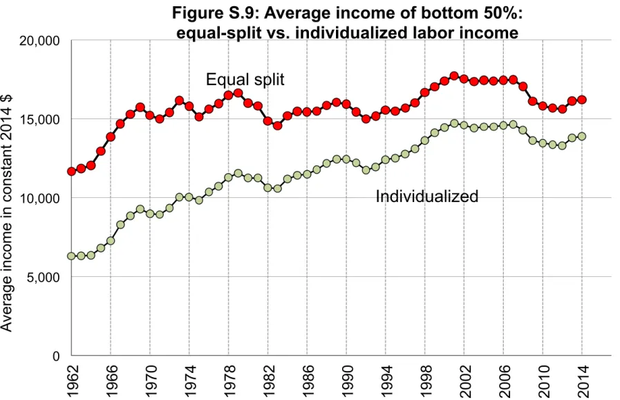
Second, top income shares studies so far were computed using the tax unit (the family in the United States, i.e. married couples or single individuals), with no adjustment at all for size. This can create various biases in levels and evolutions, e.g. an increase in the fraction of single individuals can artificially lead to an increase in inequality. So we prefer in our benchmark equal-split series to divide by two the income of married couples.

Survey-based inequality studies often use equivalence scales (such as income divided by the square root of the number of household members). In e↵ect, this would lead to series that would be intermediate between tax-unit series and our equal-split individual series (which we will compare later in the paper, so that one can very easily assess the e↵ect of the unit of observation on inequality trends). We prefer however not to use explicit non-linear equivalence scales, since they are somewhat arbitrary and introduce non-linearities in our growth decomposition exercises that are difficult to justify.

Third, the family tax unit (as used, e.g., in Piketty and Saez 2003, and Saez and Zucman

22_{We include the institutionalized population in our base population. This includes prison inmates (about} 1% of adult population in the US); population living in old age institutions (about 0.6% of adult population) and mental institutions; and the homeless population. Institutionalized population is generally not covered by surveys, so BEA removes income of institutionalized households from NIPA aggregates to construct their distributional accounts (see Furlong, 2014). We prefer to take everybody into account and allocate zero or small pre-tax income to institutionalized households (see on-line files).