HAL Id: hal-00164789
https://hal.archives-ouvertes.fr/hal-00164789
Submitted on 5 Apr 2008
HAL is a multi-disciplinary open access
archive for the deposit and dissemination of
sci-entific research documents, whether they are
pub-lished or not. The documents may come from
teaching and research institutions in France or
abroad, or from public or private research centers.
L’archive ouverte pluridisciplinaire HAL, est
destinée au dépôt et à la diffusion de documents
scientifiques de niveau recherche, publiés ou non,
émanant des établissements d’enseignement et de
recherche français ou étrangers, des laboratoires
publics ou privés.
On the Influence of Selection Operators on
Performances in Cellular Genetic Algorithms
David Simoncini, Philippe Collard, Sébastien Verel, Manuel Clergue
To cite this version:
David Simoncini, Philippe Collard, Sébastien Verel, Manuel Clergue. On the Influence of Selection
Operators on Performances in Cellular Genetic Algorithms. IEEE Congress on Evolutionary
Compu-tation CEC2007, Sep 2007, singapore, Singapore. pp.4706-4713. �hal-00164789�
hal-00164789, version 1 - 5 Apr 2008
On the influence of selection operators on
performances in cellular Genetic Algorithms
D. Simoncini, P. Collard, S. Verel, M. Clergue
Abstract— In this paper, we study the influence of the selective pressure on the performance of cellular genetic algorithms. Cellular genetic algorithms are genetic algorithms where the population is embedded on a toroidal grid. This structure makes the propagation of the best so far individual slow down, and allows to keep in the population potentially good solutions. We present two selective pressure reducing strategies in order to slow down even more the best solution propagation. We experiment these strategies on a hard optimization problem, the Quadratic Assignment Problem, and we show that there is a threshold value of the control parameter for both which gives the best performance. This optimal value does not find explanation on the selective pressure only, measured either by takeover time or diversity evolution. This study makes us conclude that we need other tools than the sole selective pressure measures to explain the performance of cellular genetic algorithms.
INTRODUCTION
The selective pressure can be seen as the ability for solutions to survive in the population. When the selective pressure is high, only the best solutions survive and colonize the population, allowing less time for the algorithm to explore the search space. Thus, the selective pressure has an impact on the exploration/exploitation trade-off: When it is too low, good solutions’ influence on the population is so weak that the algorithm can’t converge and behave as a random search in the search space. When it is too strong, the algorithm converges quickly and as soon as it is stuck in a local optimum it won’t be able to find better solutions.
Cellular Genetic Algorithms (cGA) are a subclass of Evo-lutionary Algorithms in which the population is embedded on a bidimensional toroidal grid. Each cell of the grid contains one individual (solution) and the stochastic operators are applied within the neighborhoods of each cell. The existence of such small overlapped neighborhoods guarantee the prop-agation of solutions through the grid and enhance exploration and population diversity [13]. Such a kind of algorithms is especially well suited for complex problems with multiple local optima [6]. To avoid the algorithm to converge toward one local optimum, one should apply the right selective pressure on the population and find the best balance between exploitation of good solutions and exploration of the search space.
Section 1 presents a state of the art on selective pressure in cGAs and introduces two selection operators. Section 2 com-pares the influence of the selection operators on the selective pressure. Section 3 gives a description of the benchmark used to analyze the algorithms. Section 4 presents a comparative study of performance of the algorithms. Section 5 is a study on the evolution of the genotypic diversity in the populations.
Finally in section 6 we summarize and discuss the results of the paper.
I. CELLULAR GENETIC ALGORITHMS AND SELECTIVE PRESSURE
Several methods have been proposed to tune the selective pressure and deal with the exploration/exploitation trade-off in cGA. For instance, the size and shape of the cells neigh-borhoods in which the evolutionary operators are applied, has some influence. A bigger neighborhood will induce a stronger selective pressure on the population [10]. When trying to solve complex problems, with numerous local optima, one would try to slow down the convergence of the population. That is why we use in our algorithm a Von Neumann neighborhood which is the smallest symetric neighborhood that allows the convergence of the population. The shape of the grid also has an impact on the selective pressure [1], [3], [4]: thinner grids give a weaker selective pressure on the population. This solution’s weakness is that there are not enough grid shapes for a fixed size of population to allow an accurate control of the selective pressure.
The selective pressure can also be monitored by choosing an adequate selection operator.
A. Stochastic tournament selection
The stochastic tournament selection proposed by Goldberg is a binary tournament selection that doesn’t guarantee the best solution to be selected. The stochastic tournament of rater chooses two solutions from the neighborhood of a cell
and selects the best one with probability1 − r (the worst one
with probabilityr). Real parameter r should be in [0; 1].
Given the definition of selective pressure, this selection operator explicitely gives a weaker selective pressure for
increasing r values. As r is getting closer to 1, worse
solutions increase their chances to be maintained in the population, which means the selective pressure is getting weaker.
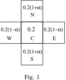
B. Anisotropic selection
The Anisotropic selection is a selection method in which the neighbors of a cell may have different probabilities to be selected [12]. The Von Neumann neighborhood of a cell C is defined as the sphere of radius 1 centered at C
in manhattan distance. The Anisotropic selection assigns different probabilities to be selected to the cells of the Von Neumann neighborhood according to their position. The
probability pc to choose the center cell C remains fixed at
1
(N ) or South (S) and pew the probability of choosing the
cells East (E) or West (W ). Let α ∈ [−1; 1] be the control
parameter that will determine the probabilitiespns andpew.
This parameter will be called the anisotropic degree. The
probabilitiespns andpew can be described as:
pns= (1 − pc) 2 (1 + α) pew = (1 − pc) 2 (1 − α)
Thus, when α = −1 we have pew = 1 − pc and pns = 0.
Whenα = 0, we have pns= pew and whenα = 1, we have
pns= 1 − pc andpew= 0. In the following, the probability
pc remains fixed at 15. C N E W S 0.2(1+α) 0.2(1+α) 0.2 0.2(1−α) 0.2(1−α) Fig. 1
VONNEUMANN NEIGHBORHOOD WITH PROBABILITIES TO CHOOSE EACH NEIGHBOR
Figure 1 shows a Von Neumann Neighborhood with the
probabilities to select each cell as a function ofα.
The Anisotropic Selection operator works as follows. For
each cell it selects k individuals in its neighborhood (k ∈
[1; 5]). The k individuals participate to a tournament and
the winner replaces the old individual if it has a better
fitness or with probability 0.5 if the fitnesses are equal.
When α = 0, the anisotropic selection is equivalent to a
standard tournament selection and when α = 1 or α = −1
the anisotropy is maximal and we have an uni-dimensional neighborhood with three neighbors only. In the following,
considering the grid symmetry, we will consider α ∈ [0; 1]
only: whenα is in the range [-1;0] making a rotation of 90◦
of the grid is equivalent to consideringα in the range [0;1].
II. TAKEOVER TIME
A common analytical approach to measure the selective pressure is the computation of the takeover time [9] [14]. It is the time needed for the best solution to colonize the whole population when the only active evolutionary operator is selection [5]. When the takeover time is short, it means that the best solution’s propagation speed in the population is high. So, worse solutions’ life time in the population is short and thus the selective pressure is strong. On the other hand, when the takeover time is high, it means that the best solution colonizes slowly the population, giving a longer lifetime to worse solutions. In that case, the selective pressure is low. So the selective pressure in the population is inversely proportionnal to the takeover time.
In order to measure the takeover time, we place one
solution of fitness1 on a 20 × 20 grid. All the other solutions
have a null fitness. Then we run the process and measure the
time needed for the solution of fitness 1 to spread over the
whole grid.
We measured average takeover times over 1000
simula-tions for a cGA using a stochastic tournament selection, and for one using the anisotropic selection. The simulations
are made on square grids of side 20. Figure 2 shows the
results of these simulations. The takeover time increases whenα increases in the case of a cGA using the anisotropic
selection (figure 2(a)). So the selective pressure is inversely
proportional toα. On figure 2(b) we can see that the takeover
time increases as long as the probabilityr to select the worst
solution in the stochastic tournament grows. This means that the selective pressure in the population is inversely
proportional to r for a cGA using a stochastic tournament
selection.
The slope of the curve representing the takeover time as
a function of α (fig. 2(a)) for values close to 1 is more
important than the one of the curve representing the takeover
time as a function of r (fig. 2(b)). We can also notice that
in the case of a cGA using stochastic tournament selection, the takeover time is defined when the probability to select
the best solution is 0. The best solution still can colonize
the population in this case since the two candidates for the tournament are selected by a random draw with replacement. In the case of a cGA using anisotropic selection, the takeover
time is not defined forα = 1.The anisotropic degree α is a
continuous parameter and the curve representing the takeover
time as a function ofα is not bounded.
III. THEQUADRATICASSIGNMENTPROBLEM
This section presents the Quadratic Assignment Problem (QAP) which is known to be difficult to optimize. The QAP is an important problem in theory and practice as well. It was introduced by Koopmans and Beckmann in 1957 and is a model for many practical problems [7]. The QAP can be described as the problem of assigning a set of facilities to a set of locations with given distances between the locations and given flows between the facilities. The goal is to place the facilities on locations in such a way that the sum of the products between flows and distances is minimal.
Given n facilities and n locations, two n × n matrices
D = [dij] and F = [fkl] where dij is the distance between
locations i and j and fkl the flow between facilities k and
l, the objective function is: Φ =X
i
X
j
dp(i)p(j)fij
where p(i) gives the location of
fa-cility i in the current permutation p.
Nugent, Vollman and Ruml proposed a set of problem instances of different sizes noted for their difficulty [2]. The instances they proposed are known to have multiple local optima, so they are difficult for a genetic algorithm.
20 40 60 80 100 120 140 160 180 200 220 0 0.1 0.2 0.3 0.4 0.5 0.6 0.7 0.8 0.9 1 Takeover Time alpha (a) 20 40 60 80 100 120 140 160 0 0.2 0.4 0.6 0.8 1 Takeover Time r (b) Fig. 2
AVERAGE TAKEOVER TIMES FOR A CGAUSING ANISOTROPIC SELECTION(A)AND STOCHASTIC TOURNAMENT SELECTION(B)
We experiment our algorithm on the instances nug30 (30 variables), tho40 (40 variables) and sko49 (49 variables) from QAPLIB.
Set up
We use a population of 400 individuals placed on a
square grid (20 × 20). Each individual is reprensented by a
permutation ofN where N is the size of an individual. The
algorithm uses a crossover that preserves the permutations:
• Select two individualsp1 andp2as genitors.
• Choose a random position i.
• Find j and k so that p1(i) = p2(j) and p2(i) = p1(k).
• exchange positionsi and j from p1and positionsi and
k from p2.
• repeatN/3 times this procedure where N is the size of
an individual.
This crossover is an extended version of the UPMX crossover proposed in [8]. The mutation operator consist in randomly selecting two positions from the individual and
TABLE I
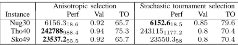
AVERAGE PERFORMANCE ANDTAKEOVER TIMES FORαoANDro
Anisotropic selection Stochastic tournament selection Instance Perf Val TO Perf Val TO Nug30 6156.318.6 0.92 65.7 6152.618.5 0.85 79.6
Tho40 242788988.4 0.94 75.3 2431151177.2 0.8 70.4
Sko49 23537.255.5 0.92 65.7 23550.358 0.8 70.4
exchanging those positions. The crossover rate is 1 and we do a mutation per individual. We perform 200 runs for each tuning of the two selection operators. An elitism replacement procedure guarantees the individuals to stay on the grid if they are fitter than their offspring. Each run stops after 2000 generations for nug30 and tho40, and after 3000 generations for sko49.
IV. PERFORMANCES
In this section we present performance results on the Quadratic Assignment Problem for a cGA using stochastic tournament and anisotropic selection operators. In [11] the
authors show that there is an optimal value of α parameter
for the anisotropic selection that gives optimal performance. We want to see if the same behaviour is observed with the stochastic tournament selection and then to compare the performance obtained for these two operators.
Figures 3, 4 and 5 show performance obtained with the anisotropic and the stochastic selection operator on the QAP instances nug30, tho40 and sko49. We measure the performance by averaging the best solution found on each run for each value of anisotropy degree and stochastic rate. When the rate of the stochastic tournament selection and the anisotropic degree are null, the two algorithms are the same : A standard cGA with binary tournament selection. The selective pressure drops when the values of the control parameters of the two algorithms increase. In both cases we see that as the selective pressure drops, performance increases until a threshold value. Once this value is reached, the performance decreases. These threshold values give the best exploration/exploitation trade-off for this problem. In
the following, the threshold values of parameters α and r
are denotedαo andro.
Table 1 gives αo and ro for each instance of QAP and
their corresponding takeover times (TO). Best performances are in bold and differences between performances of the two algorithms are statistically significant for each instance according to the Student’s t-test. Differences in takeover times are also statistically significant. The algorithm using stochastic tournament selection is the best for nug30, and the one using anisotropic selection is the best for tho40 and sko49. The threshold values stand in the same ranges
for all instances: αo ∈ {0.92, 0.94} and ro ∈ {0.8, 0.85}.
The differences in takeover times indicate that the selective pressure on the population is different for the two methods for the settings that give the best average performance. These differences can be explained by the way the algorithm explores the search space and exploits good solutions.
6155 6160 6165 6170 6175 6180 0 0.2 0.4 0.6 0.8 1 Cost alpha (a) 6150 6155 6160 6165 6170 6175 6180 0 0.2 0.4 0.6 0.8 1 Cost r (b) Fig. 3
PERFORMANCE OF CGAWITH ANISOTROPIC SELECTION FOR DIFFERENT ANISOTROPY DEGREES(A)AND WITH STOCHASTIC TOURNAMENT FOR
DIFFERENT RATES(B)ON INSTANCE NUG30
V. DIVERSITY
In this section, we present statistic measures on the evolu-tion of the genotypic diversity in the populaevolu-tion. Three kinds of measures are performed : The global average diversity, the vertical/horizontal diversity and the local diversity. The
global average diversity measure is made on a set of50 runs
of one instance of QAP for each kind of algorithm. It consists in computing the genotypic diversity between each solutions generation after generation.
gD = ( 1 ♯r♯c) 2 X r1,r2 X c1,c2 d(xr1c1, xr2c2)
whered(x1, x2) is the distance between solutions x1andx2.
The distance used is inspired from the Hamming distance: It is the number of locations that differ between two solutions
divided by their lengthn.
The results for each generation are averaged on 50 runs.
We obtain a curve representing the evolution of the global
242600 242800 243000 243200 243400 243600 243800 244000 244200 0 0.2 0.4 0.6 0.8 1 Cost alpha (a) 243000 243200 243400 243600 243800 244000 244200 244400 244600 244800 245000 245200 0 0.2 0.4 0.6 0.8 1 Cost r (b) Fig. 4
PERFORMANCE OF CGAWITH ANISOTROPIC SELECTION FOR DIFFERENT ANISOTROPY DEGREES(A)AND WITH STOCHASTIC TOURNAMENT FOR
DIFFERENT RATES(B)ON INSTANCE THO40
diversity in the population through2000 generations.
The vertical/horizontal diversity measures the average di-versity in the columns and in the rows of the grid. The vertical (resp. horizontal) diversity is the sum of the average distance between all solutions in the same column (resp. row) divided by the number of columns (resp. rows):
vD = 1 ♯r 1 ♯c2 X r X c1,c2 d(xrc1, xrc2) hD = 1 ♯c 1 ♯r2 X c X r1,r2 d(xr1c, xr2c)
where♯r and ♯c are the number of rows and columns in
the grid.
This measure is only made for the cGA with anisotropic selection. As the stochastic tournament selection provides an isotropic diffusion of solutions, the difference between horizontal and vertical diversities is null.
23530 23540 23550 23560 23570 23580 23590 23600 23610 0 0.2 0.4 0.6 0.8 1 Cost alpha (a) 23550 23560 23570 23580 23590 23600 23610 23620 23630 0 0.2 0.4 0.6 0.8 1 Cost r (b) Fig. 5
PERFORMANCE OF CGAWITH ANISOTROPIC SELECTION FOR DIFFERENT ANISOTROPY DEGREES(A)AND WITH STOCHASTIC TOURNAMENT FOR
DIFFERENT RATES(B)ON INSTANCE SKO49
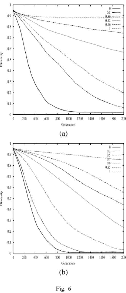
Figure 6 shows the evolution of global diversity for different settings of the anisotropic selection (fig 6(a)) and the stochastic tournament selection (fig 6(b)). Curves on
figure 6(a) represent diversity for increasing values ofα from
bottom to top. These curves show that the moreα is high, the
more the diversity is maintained in the population. Similar results are obtained in the case of the stochastic tournament on figure 6(b). These curves represent diversity for increasing
values ofr from bottom to top. The shape of the curves are
different for the two methods: For the stochastic tournament, the curves are concave in a first time and then become
convex. For high values of r, the concave phase is longer
and it is not finished at generation2000 for values above 0.8.
For the anisotropic selection, the convexity does not change, the curves are convex.
The differences in the evolution of genotypic diversity are shown on figure 7. This figure present the evolution of the
di-versity for the threshold values of the two algorithms:αoand
0 0.1 0.2 0.3 0.4 0.5 0.6 0.7 0.8 0.9 1 0 200 400 600 800 1000 1200 1400 1600 1800 2000 Diversity Generations 0 0.8 0.86 0.92 0.96 1 (a) 0 0.1 0.2 0.3 0.4 0.5 0.6 0.7 0.8 0.9 1 0 200 400 600 800 1000 1200 1400 1600 1800 2000 Diversity Generations 0 0.2 0.5 0.7 0.8 0.85 1 (b) Fig. 6
EVOLUTION OF GLOBAL DIVERSITY FOR A CGAUSING ANISOTROPIC SELECTION(A)AND STOCHASTIC TOURNAMENT SELETION(B)ON
INSTANCE NUG30
ro. We can see that the diversity is higher for the algorithm
using the stochastic tournament selection. Nevertheless, since the curve of the stochastic tournament is concave and the curve of the anisotropic selection convex, the difference of
diversity starts to decrease around generation 1000 and at
generation2000 the algorithm using anisotropic selection has
preserved more diversity.
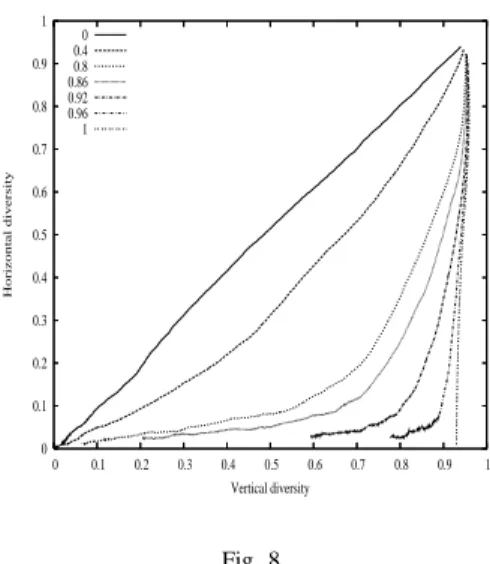
On figure 8, the horizontal diversity is plotted as a function of the vertical diversity for different settings of anisotropic
selection. The straight line is the curve obtained for α = 0
andα is increasing on curves from the left to the right. As α
increases, the algorithm favors the propagation of solutions in the columns of the grid and the vertical diversity decreases quicker. On the other hand the horizontal diversity decreases
slower, and is constant for the limit case α = 1. In the
latter case, there are no interactions between the columns of the grid and the algorithm behave as several independant algorithms executing in parallel. These algorithms run on
0.55 0.6 0.65 0.7 0.75 0.8 0.85 0.9 0.95 1 0 200 400 600 800 1000 1200 1400 1600 1800 2000 Diversity Generations anisotropic stochastic Fig. 7
EVOLUTION OF GLOBAL DIVERSITY FORαoANDroON INSTANCE
NUG30 0 0.1 0.2 0.3 0.4 0.5 0.6 0.7 0.8 0.9 1 0 0.1 0.2 0.3 0.4 0.5 0.6 0.7 0.8 0.9 1 Horizontal diversity Vertical diversity 0 0.4 0.8 0.86 0.92 0.96 1 Fig. 8
HORIZONTAL DIVERSITY AS A FUNCTION OF VERTICAL DIVERSITY FOR DIFFERENT SETTINGS OF A CGAUSING ANISOTROPIC SELECTION ON
INSTANCE NUG30
neighborhoods.
The local diversity measure is computed on one single run for each kind of algorithm. It is the genotypic diversity observed in the neighborhood of each cell of the grid. It is represented as “snapshots” of the population, where a dark point represents a high degree of diversity in the neighborhood, and a clear point represents a low degree of diversity in the neighborhood.
Figure 9 represents the local diversity along generations for a cGA with standard binary tournament selection. We can
see on snapshots of generations300 and 500 the formation of
circles. Each circle contains copies of good solutions found locally. The frontier between the areas from which good solutions colonize the grid are the only sites on the grid where the crossover operator still can have some effect. At
generation 1000 the genotypic diversity on the grid is null
, the population has been colonized by one solution, and performance will not improve anymore.
Figure 10 represents the local diversity along generations for a cGA with stochastic tournament selection. The prob-ability of selecting the best participant to the tournament is decreasing from top to bottom. The first thing we notice is that the propagation mode of good solutions is the same as for the cGA using a standard binary tournament selection. The only difference is the speed of propagation of good
solutions monitored by the r parameter. As long as we
give less chances to the best solution in the neighborhood to be selected, it will take more time before the algorithm converges. The areas where crossovers can help to explore the search space and to improve performance are bigger when r increases. The crossover operator does not have
any effect in the white zones of the grid since there is no
more genotypic diversity in such areas. For r = 1, we see
that at generation 1500 the diversity is still very high and
the algorithm does not exploit good solutions because the selective pressure on the population is too low.
Figure 11 represents the local diversity along generations
for a cGA with anisotropic selection. Values of α increase
from top to bottom. By monitoring the anisotropy degree, we can influence on the dynamics of propagation of good
solutions. For low values of α, good solutions roughly
propagate in circles as for a cGA using binary tournament
selection. When α reaches values close to 1, the good
solutions tend to colonize the columns of the grid. The diversity is conserved between the columns, which indicate that the algorithm converge toward different solutions in each columns. Thus, the anisotropic selection favors the formation of subpopulations in the columns of the grid [11]. Crossovers between subpopulations then allow the algorithm to explore the search space, as long as the probability of selecting participants from different columns for the tournament is
not too low (i.e.α is not too high). When α is too high, the
selective pressure on the population is too low and negatively affects performance.
VI. DISCUSSION
In this section we summarize and discuss the results on takeover time, performance and genotypic diversity and we compare the cGAs using anisotropic selection and stochastic tournament selection. Two cGAs using different selection operators have been tested on instances of QAP. The two selection operators allow to control the selective pressure on the population. The analysis of takeover time and genotypic diversity show the influence of the two operators on the selective pressure.
When looking at the performance on QAP, we can see that on each instance and for both methods, the performance in-creases as the selective pressure drops down until a threshold value of the control parameter. After this value, the perfor-mance decreases as the selective pressure continue to drop down. The threshold values of the control parameter stand in the same range on all instances for both of the methods.
Nevertheless, we notice from table 1 that the takeover times
are not similar for αo and ro. Consequently, the selective
pressure induced on the population is different for the two algorithms. The observations on figure 7 are in adequation with this: The algorithm with stochastic tournament preserves more genotypic diversity for the threshold value than the one with anisotropic selection. The genotypic diversity measures were made on instance nug30 for which the cGA with stochastic tournament selection obtains the best performance. However, results on diversity put in evidence properties of the selection operators which are independant from the instance tested.
The selective pressure is related to the
explo-ration/exploitation trade-off. We conclude from the
results presented in table 1 and figure 6 that studying the exploration/exploitation trade-off is insufficient to explain performance of cellular genetic algorithms. In cGAs, the grid topology structures the search dynamic.
1 300 500 1000 1500
Fig. 9
LOCAL DIVERSITY IN THE POPULATION ALONG GENERATIONS(LEFT TO RIGHT)FOR A CGAWITH STANDARD TOURNAMENT SELECTION
1 300 500 1000 1500
0.3
0.85
1
Fig. 10
LOCAL DIVERSITY IN THE POPULATION ALONG GENERATIONS(LEFT TO RIGHT)FOR INCREASINGrVALUES OF STOCHASTIC TOURNAMENT(TOP TO BOTTOM) 1 200 500 1000 1500 0.4 0.92 0.98 Fig. 11
The overlapped neighborhoods allow to control the diffu-sion of phenotypic and genotypic informations through the population.
Figures 10 and 11 show that the algorithm with stochastic tournament or anisotropic selection exploit differently the structure of the grid. When using the anisotropic selec-tion, the algorithm can favor the propagation of solutions vertically. This structuration creates subpopulations in the columns of the grid, and solutions can occasionally share information with adjacent subpopulations. On the other side, the stochastic tournament selection provides an isotropic propagation of solutions. The algorithm can control the speed of the propagation by decreasing the probability to select the best participant to the tournament as genitor. The snapshots and the figures 6 and 7 show that the genotypic diversity in the population is influenced by the exploitation of the grid structure.
The selection operator plays an important role in the explo-ration of the search space and in the exploitation of solutions. The two operators we compare allow to control the selective
pressure. For ro and αo the selective pressure induced on
the population gives the best ratio between exploration and exploitation. But this ratio is dependant of the exploration and exploitation dynamics of the algorithm. Thus, it is dependant of the selection operator used. The measures on genotypic diversity and the snapshots show these differences whether the algorithm uses the stochastic tournament or the anisotropic selection. Thus, the selective pressure needed to find the best exploration/exploitation trade-off is dependant of the transmission mode of information through the grid. Furthermore, the existence of a threshold value for the parameter which controls the selective pressure do not find explanation in the statistic measures on genotypic diversity and takeover time.
A study of the relations between topologic, phenotypic and genotypic distances should give a better explanation of performance and as a consequence should explain the takeover time and diversity during the search process. In order to explain performance of cGAs, we need to study the transmission mode of the informations through the grid since the ratio between exploration and exploitation seems to rely on it.
CONCLUSION AND PERSPECTIVES
This paper presents a comparative study of two selection operators, the anisotropic selection and the stochastic tour-nament selection, that allow a cellular Genetic Algorithm to control the selective pressure on the population. A study on the influence of the selection operators on the selective pressure is made by measuring the takeover time and the genotypic diversity. We analyse the average performance obtained on three instances of the well-known Quadratic Assignment Problem. A threshold value for the parameters of both of the selection operators that gives optimal per-formance has been put in evidence. These threshold values give the adequate selective pressure on the population for the QAP. However, the selective pressure is different for
the two methods. A study on the genotypic diversity shows that the dynamic of diffusion of informations through the grid is different when using the stochastic tournament or the anisotropic selection operator. The anisotropic selection favors the formation of subpopulations in the columns of the grid, whereas the stochastic tournament selection slows down the propagation speed of the good solutions. The selection operator have some influence on the dynamic of transmission of the information through the grid and the ratio between exploration and exploitation is not sufficient to explain the performance of a cGA.
Nevertheless, we show that even if it is different for the anisotropic selection and the stochastic tournament selection, the selective pressure has some influence on performances. Further works will analyze the dynamic of diffusion of the information through the grid and explain the existence of a threshold value for the two cGAs by studying statistic measures on the relations between topologic, genotypic and phenotypic distances.
REFERENCES
[1] E. Alba and J. M. Troya. Cellular evolutionary algorithms: Evaluating the influence of ratio. In PPSN, pages 29–38, 2000.
[2] J. R. C.E. Nugent, T.E. Vollman. An experimental comparison of techniques for the assignment of techniques to locations. Operations
Research, 16:150–173, 1968.
[3] M. Giacobini, E. Alba, A. Tettamanzi, and M. Tomassini. Modeling selection intensity for toroidal cellular evolutionary algorithms. In
GECCO, pages 3–11, 2004.
[4] M. Giacobini, A. Tettamanzi, and M. Tomassini. Modelling selection intensity for linear cellular evolutionary algorithms. In P. L. et al., editor, Artificial Evolution, Sixth International Conference, Evolution
Artificielle, EA 2003, Lecture Notes in Computer Science, pages 345–
356, Marseille, France, October 2003. Springer.
[5] D. E. Goldberg and K. Deb. A comparative analysis of selection schemes used in genetic algorithms. In FOGA, pages 69–93, 1990. [6] K. A. D. Jong and J. Sarma. On decentralizing selection algorithms.
In ICGA, pages 17–23, 1995.
[7] T. Koopmans and M. Beckmann. Assignment problems and the location of economic activities. Econometrica, 25(1):53–76, 1957. [8] V. V. Migkikh, A. P. Topchy, V. M. Kureichik, and A. Y. Tetelbaum.
Combined genetic and local search algorithm for the quadratic assign-ment problem.
[9] G. Rudolph. On takeover times in spatially structured populations: Array and ring. Proceedings of the SecondAsia-Pacific Conference
on Genetic Algorithms and Applications (APGA ’00), pages 144–151,
2000.
[10] J. Sarma and K. A. De Jong. An analysis of the effects of neighborhood size and shape on local selection algorithms. In PPSN, pages 236–244, 1996.
[11] D. Simoncini, P. Collard, S. Verel, and M. Clergue. From cells to islands: An unified model of cellular parallel genetic algorithms. In S. E. Yacoubi, B. Chopard, and S. Bandini, editors, ACRI 2006,
7th International Conference, pages 248–257, Perpignan, France, sept
2006. Lecture Notes in Computer Science 4173.
[12] D. Simoncini, S. Verel, P. Collard, and M. Clergue. Anisotropic selection in cellular genetic algorithms. In M. K. et al., editor,
Genetic and Evolutionary Computation – GECCO-2006, pages 559–
566, Seatle, 8-12 July 2006. ACM.
[13] P. Spiessens and B. Manderick. A massively parallel genetic algorithm: Implementation and first analysis. In ICGA, pages 279–287, 1991. [14] J. Sprave. A unified model of non-panmictic population structures in
evolutionary algorithms. Proceedings of the congress on Evolutionary