HAL Id: hal-01276592
https://hal.archives-ouvertes.fr/hal-01276592
Preprint submitted on 19 Feb 2016
HAL is a multi-disciplinary open access
archive for the deposit and dissemination of
sci-entific research documents, whether they are
pub-lished or not. The documents may come from
teaching and research institutions in France or
L’archive ouverte pluridisciplinaire HAL, est
destinée au dépôt et à la diffusion de documents
scientifiques de niveau recherche, publiés ou non,
émanant des établissements d’enseignement et de
recherche français ou étrangers, des laboratoires
Historical Hamiltonian Dynamics: symplectic and
covariant
M Lachieze-Rey
To cite this version:
Historical Hamiltonian Dynamics: symplectic and
covariant
M. Lachi`eze-Rey,
APC - Astroparticule et Cosmologie (UMR 7164)
Universit´e Paris 7 Denis Diderot 10, rue Alice Domon et L´eonie Duquet
F-75205 Paris Cedex 13, France
[email protected]
February 19, 2016
Abstract
This paper presents a “ historical ” formalism for dynamical systems, in its Hamiltonian version (Lagrangian version was presented in a previous paper). It is universal, in the sense that it applies equally well to time dynamics and to field theories on space-time. It is based on the notion of (Hamiltonian) histories, which are sections of the (extended) phase space bundle. It is developed in the space of sections, in contradistinction with the usual formalism which works in the bundle manifold.
In field theories, the formalism remains covariant and does not require a spitting of space-time. It considers space-time exactly in the same manner than time in usual dynamics, both being particular cases of the evolution domain. It applies without modification when the histories (the fields) are forms rather than scalar functions, like in electromagnetism or in tetrad general relativity.
We develop a differential calculus in the infinite dimensional space of his-tories. It admits a (generalized) symplectic form which does not break the covariance. We develop a covariant symplectic formalism, with generalizations of usual notions like current conservation, Hamiltonian vector-fields, evolution vector-field, brackets, ... The usual multisymplectic approach derives form it, as well as the symplectic form introduced by Crnkovic and Witten in the space of solutions.
1
Introduction
Our historical Hamiltonian formalism is based on the notion of history. Ac-cording to [24], histories “ furnish the raw material from which reality is con-structed”.
This follows our previous work ([6], hereafter paper I) which presents a Lagrangian formalism on the same basis (see an outline in Appendix A). An history (or kinematical history) is a possible evolution of a dynamical system, also called a configuration [18]. An history which obeys the dynamical equations becomes a physical evolution, or particular solution.
Our approach applies equally well to usual time dynamics (tD) and to co-variant field theories (FT), and allows further generalizations. These different contexts (tD and FT) only differ by their evolution domain (see below): the time line in tD; the space-time in FT. But all expressions or equations are iden-tical in both cases. Thus space-time in FTs appears on the same footing than time in tD, with the only difference that it is 4 dimensional rather than mono-dimensional. In the case of FTs, our formalism remains entirely covariant and does not require any splitting of space-time.
In addition, it applies without modification to the case where the fields are not functions, but forms (e.g., on space-time). This applies to electromagnetism or to general relativity in the tetrad formalism.
In paper I, we have presented its Lagrangian version. Here we present the Hamiltonian one. The most important result is the existence of a canonical (gen-eralized) symplectic form which remains entirely covariant. In time dynamics, it is equivalent to the usual symplectic form. In field theories, it remains covariant and we show that the multisymplectic formalism may be seen as derived from it. To mention some general ideas underlying this approach,
• dynamics is defined, not versus time but versus an evolution domain. It reduces to the time line in tD (a particular case); to space-time for FT’s. But it is treated exactly in the same manner in both cases.
• An history may be a function on the evolution domain (like a scalar field on space-time) but also, more generally, a differential form on it; in any case a section of a particular fiber bundle.
• A particular solution is an history which is an orbit of a [Hamiltonian] flow in the corresponding bundle. Such flows have the dimension of the evolution domain. They may be called general solutions.
• Our calculus does not hold in configuration space, or phase space, but in the space of histories which has infinite dimension It is inspired by diffeology [14] considerations. It may be seen as generalization of both [29] and the multisymplectic formalism, and as a synthesis between them. • In the space of (Hamiltonian) histories, we define a canonical and covariant (generalized) symplectic form; equivalent to the usual symplectic form in tD; giving raise to both the multisymplectic form and the symplectic currents [29] in FTs.
• Covariant field theories (in space-time) and time dynamics appear as two particular cases of this formalism.
In some sense, our formalism appears as a generalized synthesis between the multisymplectic geometry (see, e.g., [11]), the “ covariant phase space ”ap-proaches (see, e.g., [11]), the canonical approach and the geometry of the space of solutions. It remains entirely covariant.
The section 2 introduces the notion of history (2.1). It defines their prolonga-tions to velocity-histories and Hamiltonian histories, involved in the Lagrangian and Hamiltonian formulations of dynamics, and introduces the phase space bun-dle (2.2). It also explicits our differential calculus in the space of Hamiltonian Histories (2.4). Section 3 expresses the Hamiltonian Dynamics in its historical
formulation. It introduces the generalized symplectic form and the evolution H-vector field (3.1). It derives the universal historical evolution equations (3.2) and explicits the dynamical solution (3.3). Section 4 gives illustrations, apply-ing the general formalism to time Dynamics (4.1), and to scalar field theories, where our formalism is compared to the multisymplectic one (4.2). Section 5 considers conservation (5.1) and symmetries (5.2) It discusses the notions of [generalized] Poisson brackets and observables (5.3). The last sections apply to electromagnetism (6) and to first order general relativity (7). An outline of the historical Lagrangian formalism presented in paper I is given in Appendix A.
2
General framework
Our framework applies equally well to (non relativistic) time dynamics and to relativistic (covariant) field theories. It is formulated in terms of histories, that we define below. Shortly, an history is associated to each degree of freedom of the dynamical system. We treat only the case of an unique degree of freedom; the generalization to multicomponent-systems is straightforward and is treated in illustrations below. The case of a form-field rather than a scalar field, like the electromagnetic potential in Maxwell theory, is treated as a single degree of freedom, to which correspond an unique (although not scalar-valued) history (a 1–history); or the tetrad general relativity, where the cotetrads forms eI and
and the spin connection forms ωIJare also 1–histories. We treat first the scalar
field case and then extend to the form field.
2.1
Histories
A dynamical system is characterized by its configuration bundle C → D. Here, D is the domain of the theory. In usual time dynamics (tD), this is the time line IRt, or an interval of it. In relativistic field theories (FT), this is
space-time. We treat both cases equally, and more generally, D is a n-dimensional differentiable manifold, possibly with a given metric. We label D with arbitrary coordinates xµ (the unique coordinate t = x0 for the timeline in tD), which
disappear in our final results which are covariant 1. They generate adapted
[local] coordinates in the various fiber bundles we will consider. Our philosophy is to treat D as some kind of “ n-dimensional timeline ” w.r.t. which the evolution is expressed.
An element of the fiber is a possible value of the dynamical variable. Most physical systems admit many degrees of freedom (or components). We treat the case of an unique component. The generalization to composite fields is straightforward as it will appear in the examples below. Thus for the particle in space, an history corresponds to each coordinate as C : t → qi(t); for a scalar
field in space-time, C : (xµ) → C(xµ) generally written ϕ(xµ); for a composite
field, one history for each component φA.
An history (or field-history, or configuration), that we always write C, is a section 2 of the configuration bundle C: a function on D for the particle
or for the scalar field; but, more generally, a differential form on D like in
1
We define the non covariant forms Vol def= dnx, Vol µ
def
= ∂µyVol and Volµα def
= ∂α, ∂µy Vol in D, as usual.
electromagnetism or in tetrad general relativity (see below). Thus, the space of histories C = Sect(C), or possibly a subset of it. The histories which obey the dynamical equations are the particular solutions.
2.2
The Phase Space Bundle and Hamiltonian Histories
Given an history C, the corresponding velocity-history is its first jet extension (or prolongation), the pair CV
def
= jC def= (C, dC) (with d the exterior derivative in D) or (C, Cµ) in components. This is a section of the first jet
bundle J C. In paper I, we have developed the Lagrangian historical formalism in this jet bundle (see A).3
Its affine dual J∗
C → C. Its bundle manifold, the phase space 4, admits
the adapted [Darboux] coordinates5 xµ, φ, pµ, π. They act by duality [18] as
h(xµ, φ, pµ, π), (xµ, φ, v
µ)i = (pµ vµ+ π) Vol.
We see the polymomenta pµ as the dual components of the (n-1)–form over D,
p def= pµ Vol
µ, that we call the polymomentum6.
The (extended) phase space bundle is the bundle Y = J∗
C → D. A section is a map
Y = (Xµ, C, P,Π) : xµ→ Xµ(xµ) = xµ, C(xµ), P (xµ), Π(xµ),
that we call an Hamiltonian history (hereafter H-history)7. The components are
expressed in the table 1, where Ωk
D= Ωk(D) is the space of k-forms on D. We
call P the historical momentum. The trivial maps Xµ, defined for convenience,
will appear as the conjugate variables to the Πµ.
Any H-history Y defines a n-dimensional hypersurface in the phase space, which is simply its image Im(Y ). And Y is a diffeomorphism D → Im(Y ) = Y(D). When the history is a solution, Im(Y ) is an orbit of the evolution flux (see below).
We will work in the space of Hamiltonian histories rather than in the phase space bundle. We first define differential calculus in it.
3
An interesting different point of view [23] considers a field configuration as a section of the infinite jet bundle J∞
C.
4 Different authors use various appellations for this bundle or for its associated manifold:
the covariant phase space bundle, the doubly extended phase space [7], the extended dual bundle [22], the extended multimomentum bundle [19], the De Donder-Weyl multisymplectic manifold ...
5For time dynamiccs, replace xµby t, φ by q, pµby p. 6
Equivalently, the pµare the components of the dual polymomentum ⋆p = pµdxµ(sum
over indices).
7
It is known that Y may also be seen as the bundle Vn 2T
∗
Qof n-forms over Q which annihilates two arbitrary vertical vector-fields, see, e.g., [11], [17]. In this case, pµ and π
appear as the coefficients in the expansion of such an n-form.
There is a canonical projection which projects it out to the linear dual [7] eY, forming the line bundle [22]
ρ: Y → eY: (xµ, ϕ, pµ, π) → (xµ, ϕ, pµ).
Interestingly [22, 3, 8], the (scalar) Hamiltonian may be seen as a section eh of that bundle, which defines the function H on eYthrough
eh(xµ, ϕ, pµ) = (xµ, ϕ, pµ, H (xµ, ϕ, pµ)) .
It is equivalent to work in Y or in eY. Both are polysymplectic. For the relation between both approaches, see also [3, 22, 8].
Table 1: The components of an hamiltonian history C D → Ω0 D (xµ) → C(xµ) P = Pν Vol ν D → Ωn−1D (xµ) → P (xµ) Pν D → Ω0 D (xµ) → Pν(xµ) Πν D → Ωn−1D (xµ) → Πν(xµ) Π = Πν dxν D → ΩnD (xµ) → Π(xµ) Xν dxν D → Ω0 D (xµ) → Xν(xµ) = xν
2.3
Extension to form-fields
Our formalism applies equally well in the case where a field-history C is a r-form, rather than a function (0-form), on D. We treat explicitly the case r = 1. This applies to electromagnetism, where C corresponds to the Maxwell potential A; or to general relativity in tetrad formalism, where histories correspond to the cotetrad fields eI and to the connection forms ωIJ, see below. We do not
consider separately the components of a form-field, but we treat it globally as an history C as in the table 2.
The scalar case corresponds to r = 0. When r > 1, the treatment is similar, with indices replaced by multi-indices (see paper I, and appendix C). The table 2 presents the components of an Hamiltonian history in the case r = 1. In all formula, juxtaposition implies wedge product inD. We calculate now in the infinite dimensional space Y of Hamilton–histories.
Table 2: The components of an hamiltonian history
C= Cαdxα D → ΩrD (xµ) → C(xµ) = Cα(xµ) dxα
P= PµαVol
2.4
Differential Calculus with Hamiltonian histories
An Hamiltonian history (H-history) Y is a section of the bundle Y. We call Y the infinite dimensional space of H-histories, and we construct differential calculus on it8. We represent such a section (a H-history, a “ point ” of Y) as
Y = (X, C, P, Π) = (YA),
where we treat the YA = X, C, P, Π (with A = 1, 2, 3, 4) like four coordinates
in Y9.
We generalize the notions of functions, vector-fields, differential forms... to H-maps, H-vector-fields, H-forms. This appears necessary to define a correct calculus. A H–map is an application
F : Y → Ω(M ) : Y = (YA) → F (Y ) = F (YA).
When F (Y ) ∈ ΩR(M ), we call F a [0;R]-map. The Hamiltonian functional H
will appear as a particular [0,n]–map. We write C(Y) = Ω0(Y) the space of
H-maps.
Hereafter, juxtaposition of H-maps will mean their wedge product on D, always implicit. This gives to C(Y) an algebra structure. Also, the differential calculus on D is easily lifted to Y through the formula
(dF )(Y ) = d(F (Y )).
We call occasionally d the horizontal derivative, but we do not consider it as part of the proper differential calculus on Y. We introduce below a genuine external derivative D in Y, different from d and commuting with it. This is analog to the double complex structure introduced by [4].
2.4.1 Derivations are vector-fields
We first define derivations of H-maps w.r.t. their arguments YA, under the form
of basic partial derivative operators ∂A= ∂Y∂Aacting on Y. This is accomplished through the variation formula (wedge product in D assumed)
δF = ∂F ∂YA δY A= ∂F ∂X δX+ ∂C ∂X δC+ ∂F ∂P δP+ ∂F ∂Π δΠ (1) = ∂F ∂Xµ δX µ+ ∂C ∂X δC+ ∂F ∂P δP+ ∂F ∂Πµ δΠµ,
corresponding to the general variation of a H-history δY = (δX, δC, δP, δΠ) = (δYA).
We call the operators ∂A the basic vector-fields in Y. The general
H-vector-field on Y is V = VA ∂
A, whose components VA ∈ C(Y) are arbitrary
H-maps. It acts on an H-map F , as V (F ) = VA ∂F
∂YA (wedge product in D still implicit) 10.
8
Note that similar approaches ([30], [4]) consider elements of Ω(Sect(ΩD× D). 9X holds for the four Xµ; C holds for the infinite set of values C(x) (or C
µ(x) if r 6= 0).
Our notation allows us to manage this infinite set like one unique coordinate; similarly with P .
10
2.4.2 H-forms
We define [differential] H-forms in Y through duality. First the basis one-forms DYA – which mean the collection DXµ,DC, DP, DΠ
µ – through their actions
on an arbitrary H-vector-field,
hDYA, Vi = VA. The general one-H-form expands as
α= αA DYA,
whose components αA∈ C(Y) are arbitrary H-maps (sum over repeated indices
is always assumed). We have
hα, V i = αA VA;
and the exterior derivative of a H–map F DF = ∂F
∂YA DY A.
This is just an other way to write equ.(1), after realizing that a variation of a H-history is simply the action of a H-vector-field δ = δA ∂
A on it, namely
δYA= δ(YA) = hDYA, δi = δA
(this requires δA to be of the same grade than YA). When F is a [0,R]-map, we
call DF a [1,R]-H-form; [0,R]-maps are [0,R]-H-forms.
The wedge product of H-forms, ∧ (not to be confused with the wedge product on D which is always implicit), is defined as antisymmetrized tensor product, as usual. It generates [2,R]-H-forms, etc. The external derivative D also applies to [k,R]-forms and generates [k+1,R]-forms. Thus we have the rules expressed in table 3. Contraction of H-vector-fields with H-form is as usual.
Table 3: Differentials of H-forms
( [k;R]-form) ∧ ( [k’;R’]-form) = [k+k’;R+R’]-form d ( [k;R]-form) = [k;R+1]-form ;
D ( [k;R]-form) = [k+1;R ]-form .
We have for instance
DH = ∂H ∂Xµ DX µ+∂H ∂C DY C+∂H ∂P DY P + ∂H ∂Πµ DYΠµ =∂H0 ∂C DY C+∂H0 ∂P DY P+ dxµ DYΠµ
where we used equ.(2) in the last term.
These formulas also apply equally well in the case where the histories are not scalar, i.e., [0,r]-histories rather than [0,0]-histories. We give in appendix B their explicit development for one-form valued histories, i.e., [0,1]-histories rather than [0,0]-histories. They generalize easily to the general case of [0,r]-histories. We give in table 4 the grades of the different H-maps and H-forms involved (scalar case corresponds to r = 0).
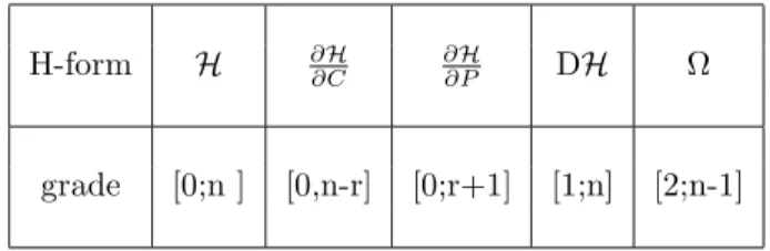
Table 4: The grades of the H-maps and H-forms
H-form H ∂H
∂C
∂H
∂P DH Ω
grade [0;n ] [0,n-r] [0;r+1] [1;n] [2;n-1]
3
Dynamics and evolution
3.1
The symplectic H-form
The space of histories Y admits the canonical [1;n-1]-Hform Θ def= P DC + Πµ DXµ= Pµ DC Volµ+ π DXµ Volµ,
that we call the Poincar´e-Cartan H-form [18]. Its [vertical] exterior derivative Ω def= DΘ = DP ∧ DC + DΠµ∧ DXµ,
is a closed and non degenerate [2;n-1]–form on Y, that we call the symplectic H–form. For a 0-history, Ω = (DPµ∧ DC) Vol
µ; for a 1-history, Ω = (DPαµ∧
DCα) Volµ. For r > 1, the same formulas hold, with indices replaced by multi–
indices. We will see below that it allows us to construct a genuine (scalar-valued) symplectic form in the space of solutions, which identifies to that of [29].
Under some conditions, a H–map F admits a symplectic gradient ∇ΩF, a
H-vector-field defined through
∇ΩF yΩ = DF.
3.2
Evolution
The Dynamics is described by the historical Hamiltonian11
H = h Vol = H0(C, P ) + Πµ dxµ. (2)
This is a [0;n]-H-map H : Y → Ωn D.
The evolution vector-field is defined as its symplectic gradient Z = ∇ΩH:
Z yΩ = DH.
We emphasize that there is no analog in the multisymplectic formalism. It expands as Z = ZA ∂
A, and the equation above gives its components through
ZAΩ
AB= ∂Y∂HB, with explicit solution ZP = −∂H ∂C, Z C= ∂H ∂P, Z Xµ = ∂H ∂Πµ = dxµ, ZΠµ = − ∂H ∂Xµ = 0 (3)
(note the difference between xµ and Xµ), where ZP and ZC are [0;n-r]- and
[0,r+1]–Hmaps respectively. This evolution vector-field acts as a derivation operator on any H–map F , giving the H–map
Z(F ) = ZA ∂F ∂YA,
with the components given in equ.(3); in particular the derivatives of the “ co-ordinates ”, Z(YA) = ZA. In particular Z(Xµ) = dxµ, Z(Πµ) = 0.
3.3
The dynamical solution
An H–history Y = (YA) is a real motion (solution) when the evolution
vector-field is tangent to it. This means dYA= Z(YA) = ZA, i.e., using (3)
dC = ∂H ∂P; dP = − ∂H ∂C, dX µ= dxµ, dΠ µ = 0. (4)
The two last are identities. We recall that d is the (horizontal) exterior derivative in D, not be confused with exterior derivative D in Y.
This “ historical ” version of the Hamilton–De Donder–Weyl equations ap-plies to tD as well to FT. We show below that it leads to the usual dynamical equations. It includes the case where the field is a form rather than a map (e.g., electromagnetism or general relativity), as we show in applications below. For a multi–component history (field) it holds for each component.
It is easy to check that the previous equations insures stationarity of the actionRD L, with the Lagrangian H–map (see paper I)
L = P dC − H. Namely, using the commutativity between d and D,
DL = D(P dC − H) = DP dC − P DdC − DH = = DP dC − ǫ(d(P DC) − dP DC) − (∂H
∂C DC + ∂H ∂P DP ).
Inserting the motion equations above, this reduces to DL = −d(P Dc), an exact form in D which gives zero contribution to the integral, QED.
4
Illustrations
4.1
Application to time Dynamics
In usual dynamics, D is the time line, Vol = dt, Π = π dt and Πµ = Πt = π.
Then
H =12 ⋆P P+ U (C) dt + π dt = h dt,
with h = 12 P P + U (C) + π the usual Hamiltonian function; C = q and P = p are zero-forms (r = 0). Then ∂H∂C = ∂C∂h dt = U′
(C) dt and ∂H∂P = ∂P∂h dt = P dt are both [0;1]-Hmaps. Ω = DP ∧ DC + DΠ ∧ DT is a [2,0]-form (a genuine scalar valued symplectic form).
Then, (4) immediately gives the usual Hamilton equations (we reintroduce the familiar notations):
dC = ˙Cdt = ∂H ∂P = ∂h ∂P dt =⇒ ˙C= ˙q = ∂h ∂p. dP = ˙P dt = −∂H ∂c = − ∂h ∂c dt =⇒ ˙p = − ∂h ∂c; with dT = ∂H ∂Πt = dt; dπ = ∂H ∂T = 0. (5)
4.2
Scalar field; Link with Multisymplectic
For classical field theories, D = M is space-time (n = 4). A scalar (r = 0) field C is usually written ϕ. Then P = Pµ Vol
µ is a [0,3]-Hmap, with dual
components Pµ, H = h
0Vol + Πµ dxµ is a [0,4]-Hmap. We have
dC = C,µdxµ, P = Pµ Volµ, dP = Pµ,α dxαVolµ= Pµ,µ Vol.
Then ∂H ∂P =
∂h
∂Pµ dxµ is a [0,1]-Hmap; ∂H∂C = ∂C∂h Vol is a [0;4]-Hmap. The symplectic [2,3]-Hform
Ω = DP ∧ DC + DΠµ∧ DXµ= DPµ∧ DC Volµ+ DΠµ∧ DXµ,
with Volµ a 3-form on space-time D = M (not on Y). Then, equ.(4) implies the
usual Hamilton equations C,µ= ∂h ∂Pµ; (P α) ,α= − ∂h ∂C.
Assuming the standard Hamiltonian for scalar field theories, H =1 2 ⋆P P+ U (C) Vol + 1 2 ⋆Πµ dx µ= (1 2 P µ P µ + U (C) Vol +12 π2) Vol, we obtain dC = C,µdxµ= ⋆P = Pµ dxµ ⇒ C,µ= Pµ; dP = −∂H ∂C = −U ′ (C) Vol =⇒ dPµVol
4.2.1 Link with Multisymplectic
The multisymplectic form appears as an emanation of our symplectic H-form, as the 5-form in the phase space bundle manifold Y (not on SY),
ΩM = − dpµ ∧ V OL− µ − ∧ − dϕ + − dπ −∧ V OL, where all forms, exterior derivative
−
d and wedge product ∧ are in the bundle− manifold Y, V OL def= ǫµαβγ − dxµ ∧− −dxα −∧ −dxβ −∧ −dxγ and V OLµ def = ǫµαβγ − dxα −∧−dxβ ∧−−dxγ. 4.2.2 Application to r-histories
Exactly the same formalism applies when fields are forms rather than scalar functions, with indices replaced by multi-indices (see C):
c= cα dxα, dc = cα,µdxαµ;
P = Pαµ Volαµ, dP = Pαµ,β Volαµ dβ, H = h Vol,
∂H ∂P = ∂h ∂Pαµ d αµ, ∂H ∂c = ∂h ∂cα Volα,
giving the Hamilton equations cα,µ= ∂h ∂Pαµ; (P αµ) ,µ= − ∂h ∂cα , where all multi-indexes are antisymmetrized.
5
Conservation and symmetries
5.1
On shell conservation
Interestingly, equ.(4) implies, on shell, DH = ∂H
∂c Dc + ∂H
∂P DP ≃ dc DP − dP Dc =⇒ DDH = 0 = Ddc DP − DdP Dc = dΩ
after derivation: the generalized symplectic form is conserved on shell. This is the covariant version of the on shell conservation of the symplectic current in the multisymplectic formalism.
Since the value of Ω is a (n − 1)-form on D, it can be integrated along a 1-codimensional hypersurface of D. This provides a canonical scalar-valued symplectic form on the space of solutions since the on–shell conservation of Ω implies that this symplectic form does not depend on the choice of the hypersur-face (assumed Cauchy for FTs). Thus, this provides a canonical (scalar valued) symplectic form on the space of histories, which identifies with that introduced by [29], so that our result may be seen as a generalization of their work and its link with the multi–symplectic formalism.
5.2
Symmetries
We recall that a solution is a H-history Y verifying Z(Y ) = dY or, in coordi-nates, ZA = dYA. Any vector-field δ (of convenient grade) defines a variation
δ(Y ) of that history. One may check immediately that the variation of a solution remains a solution, i.e., that
Z(Y ) = dY =⇒ Z(δ(Y )) = dδ(Y ).
• A symmetry is a Hamiltonian vector-field δ that preserves H: 0 = δ(H) = δ y DH = δ y (Z y DH) = −Z y (δ y ω) = ω(δ, Z). In coordinates, this implies δA ∂H
∂YA = 0. • Being Hamiltonian, δ is a symplectic gradient:
δ y ω= DU. Then
δ(H) = −Z y (DU ) = −Z(U ) = 0 : the quantity U is conserved on shell.
5.3
Generalized Poisson bracket and observables
The main result here is the introduction of the historical symplectic H–form Ω. Is it possible to define a Poisson-like bracket from it ? The formula above suggests that the canonical “ variables ” are the forms C and P and that the bracket of two Hmaps could be defined as
{f, g} = ∂f ∂C ∂g ∂P − ∂g ∂C ∂f ∂P = XfyDg, involving the multisyplectic gradient Xf such that XfyΩ = Df .
Table 5: The types of the Hmaps and Hforms involved
c P f,Df g,Dg Ω Xf {f, g}
[0; r] [0;n-r-1] [0;R],[1;R] [0;S],[1;S] [2,n-1] [-1;R+1-n] [0,S+R+1-n]
We give in table 5 the grades of the various quantities involved. The grade [-1;R+1-n] for the vector-field indicates that the inner product with a [1;K]– Hform gives a [0;R+1-n+K]–Hmap. This definition requires that the quantities involved are well defined and we restrict the validity of our bracket to such cases. This occurs when f and g have both degrees greater or equal to those of c and P , namely r and n − r − 1; or, alternatively, when f or g does not depend on the “ canonical variables ”. To illustrate, we have
{H, c} =∂H ∂P = dc; {H, P } = −∂H
∂c = dP.
These formulas validate the definition of our bracket. It is a generalization of that proposed by [15].
It is defined for Hmaps, whose values are forms, rather than scalar functions. However, an observable is generally considered as scalar-valued, not form-valued. But any form provides a scalar by integration over a submanifold of adapted dimension. Thus, it seems a convenient point of view to consider generalized ob-servables as form-valued, from which non–local scalar obob-servables are extracted through integration over intermediary submanifolds. This corresponds indeed to what is done in Loop Quantum Gravity through the introduction of the Holonomy-Flux algebra.
The observables which commute with the Hamiltonian and with the con-straints correspond to the complete observables in the sense of [20, 5] (see also [28]).
6
Application to electromagnetism
The usual treatment of electromagnetism considers the components Aµ of the
electromagnetic form A as the dynamical variables, with the scalar Lagrangian L=12 Fµν F
µν, where Fµν def
= ∂µAν− ∂νAµ. Indices are lowered / raised with
the fixed flat Minkowski metric.
1) The usual (non covariant) analysis proceeds by fixing one time coordi-nate t = x0, so that
L= F0i (∂0Ai− ∂iA0) +12 Fij (∂iAj− ∂jAi).
We obtain the conjugate momenta P0 def= ∂L
∂ ˙A0 = 0 and P
i= F0i= ∂
0Ai−∂iA0.
The first relation appears as the primary constraint P0 = 0 and the second
inverts as ∂0Ai = Pi+ ∂iA0. Applying a partial Legendre transform leads to
the Hamiltonian
H = λ P0+ ˙Ai Pi− [Pi Pi+12 Fij (∂iAj− ∂jAi)]
= λ P0+ (∂iA0) Pi−12 Fij (∂iAj− ∂jAi).
The primary constraint is second class and generates the secondary con-straint (Pi)
,i= (F0i),i= 0: the Gauss law. Finally, the motion equations give
˙
Ai = (A0)i and ˙Pi = −(F ij)j. This may be synthetized in F,νµν= 0.
2) The (covariant) multisymplectic analysis starts from the same Lagrangian and, now, associates to each variable Aµ the four polymomentum components
pµν = 1
2 (Fµν − Fνµ). They obey the constraints Cµν = pµν+ pνµ = 0. The
Hamiltonian
λµν Cµν−12 p µν p
µν,
leads to the usual equations, via a multisymplectic analysis (see, e.g.[26]). 3) Adopting our formalism, we write L = L Vol = 1
2 dA ⋆dA so that P =
⋆dA, which inverts as dA = ⋆P : there is no constraint and our Hamiltonian takes the form H = 1
This gives the motion equations dA = ∂H
∂P = ⋆P ; dP = 0, which condense into d⋆dA = 0.
7
Application to canonical gravity
7.1
Dynamics in the first order formalism
The dynamical variables are the cotetrad components eI and the Lorentz
con-nection forms ωIJ, with conjugated polymomenta P
I and ΠIJ. We calculated
them in paper I, namely PI = 0 and
ΠIJ = PIJ def
= ǫIJKLeKL. (6)
They generate primary constraints and we write the Hamiltonian H-form
H = PIVI+(ΠKL−PKL) WKL+PIdeI+ΠKLdωKL−ǫIJKLeIeJ(d ωKL+(ωω)KL)
= PI VI+ (ΠKL− PKL) WKL+ PI deI− ΠKL(ωω)KL
with the Lagrange multipliers VI and WKL.
The development of equ.(4) gives the motion equations: • deI = ∂H ∂PI = VI + deI, giving VI = 0; • dωIJ = ∂H ∂ΠIJ = WIJ− (ωω)IJ; (7) • dPI = − ∂H ∂eI = 2 ǫKLIJ e J WKL. (8)
The two latter combine to give the secondary constraint dPI = 0 = 2 ǫ
KLIJ eJ(dωKL+ (ωω)KL), leading to zero Ricci curvature;
• dΠIJ = − ∂H ∂ωIJ = 2 ǫP QK[I e P Q ωK J] = 2 ǫN KIJ eN M ωKM (9)
appears as a secondary constraint giving zero torsion, as can be checked using identities 6 and 16.
Appendices
A
Outline of paper I
A.1
Velocity–Histories
Histories and velocity-histories are defined as in the text (2.2). We call SV ⊂
Sect(V) the space of velocity-histories (technically, an exterior differential sys-tem [3]). Since J is canonical, there is a one-to-one correspondence between histories and velocity-histories.
We express the Lagrangian dynamics in SV rather than in the jet bundle
itself. We treat SV like an infinite dimensional manifold where C and dC
play the role of coordinates. We define H-maps SV → ΩD as generalizations
of functions. They form the algebra Ω0(S
V), and we have defined derivations
w.r.t. their arguments C and dC. We have also defined differential forms on SV,
forming the spaces Ωr(S
V), and an exterior derivative D : Ωr(SV) → Ωr+1(SV),
which commutes with d (occasionally called the horizontal exterior derivative). Dynamics is described through the Lagrangian functional
L : SV → ΩnD: CV def
= (C, dC) → L(CV),
a H-map over SV, of type [0,n].
We define the historical momentum P def= ∂L
∂(dC) = P
µ Vol
µ (10)
as a [0;n-r-1]-Hmap admitting the dual components Pµ. This formula is written with multi-indexes (see paper I); they reduce to ordinary indices when C is a 0-history; to an antisymmetric pair of indices when C is a 1-history.
Then, applying our differential calculus, we have (wedge products between forms in D are implicitly assumed)
DL = DC ∂L
∂C + D(dC) P = DC ( δELL
δC ) − dΘ. (11)
We have defined the EL derivative δELL δC def = ∂L ∂C − ǫc d ∂L ∂(dC), (12)
with ǫc= (−1)grade of C; and also the historical Lagrange form (or Lagrange
H-form) as the [1; n-1]-form
Θ def= − DC P = DC ∂L ∂(dC).
The latter gives by derivation the [2; n-1]-form DΘ = DP ∧ DC (implicit wedge product in D) which we call the symplectic H-form (and Θ the generalized symplectic potential). This is the historical version of the symplectic structure on TM (see, e.g.[16, 2]). 12
12
An arbitrary variation of an history is seen as the result of the application of a vector-field δ in SV as
δC= hDC, δi; δ(dC) = hD(dC), δi.
This leads to equ.(11). Since the last term in this equation does not contribute to the action, stationarity corresponds to the Euler-Lagrange equation δELL
δC = 0.
These equations are explicitely covariant. They apply equally well to tD and FT’s, and they include the case where the C is a r-history, i.e., a form rather than a function.
A.2
Symmetries
A vector-field δ is a symmetry generator when it does not modifies the action. This means that it modifies L by an exact form (in D) dX only. Hence, for a symmetry,
δC (δ
ELL
δC ) − d(δC P ) = dX.
Defining the Noether current ([n-1]-H-map) j def= X + δC P , we have the conservation law
dj = δC δ
ELL
δC ≃ 0 (on shell).
Locally, j = dQ which defines the Noether charge density (n − 2)-H-map Q [27]. A diffeomorphism of D is obviously a symmetry since in that case δL = LζL = d(ζ y L), where ζ is the generator.
The historical Legendre transform (see below) will allow the change of vari-ables (C, dC) ; (C, P ) at the basis of the Hamiltonian formalism.
A.3
Legendre transform
The (usual) Legendre transform transports the dynamics from V to Y. It is defined as the fiber-preserving map [9]
TL: V → Y : (xµ, ϕ, vµ) ; (xµ, ϕ, pµ, π),
here for a scalar field, in adapted coordinates. 13 It may be non invertible, what
is expressed by primary constraints. We assume now a non degenerate Legendre transform, constraints are discussed in the examples.
We lift the Legendre transform to the historical Legendre map which applies to sections, the duality
TL: SV → Y : C = (C, dC) ; Y = (C, P )
between velocity-histories and Hamiltonian histories. This results from the sim-ple remark that a fiber-preserving map between fiber bundles induces a map between their spaces of sections. Concretely, the velocity history CV is
trans-formed, by composition with TL, as Y = TL◦ CV. 13It admits a restricted version
V ; eY: (xµ, ϕ, v
A.4
The historical Hamiltonian
We define the historical Hamiltonian on the historical phase space
H : Y → Ωn(D) : Y → H(Y ) = Λi Γi+ Π Vol + P dC − L (13)
(wedge product assumed). In this expression, dC and L are expressed as func-tionals of C and P , as far as allowed by inversion of the Legendre map, so that H is a [0;n]–Hmap. The Λiand Γ
iare Lagrange multipliers and constraints, which
are now defined as Hmaps also (see illustrations in examples). This definition holds for r–histories.
B
Details of Calculations
• For a scalar field, a field-history is a zero-form C on D. The momentum is a 3 form P = Pµ Vol
µ (its Hodge dual ⋆P = Pµ dxµ is a 1-form).
The Hamiltonian functional is a [0;4]-H-map H = h Vol. Its external derivative DH = ∂H ∂C DC + ∂H ∂P DP... = ∂h ∂C DC Vol + ∂h ∂Pµ DP µ Vol..., so that ∂H ∂C = ∂h ∂C Vol, ∂H ∂P = ∂h ∂Pµ dx µ.
• For a one-form field, a field–history is a one form C = Cαdxαon D. The
momentum is a 2 form P = PαµVol αµ.
The Hamiltonian is a [0;4]-H-map H = h Vol. Its external derivative DH = ∂H ∂C DC + ∂H ∂P DP... = ∂h ∂Cα DCαVol + ∂h ∂Pαµ DP αµ Vol..., so that ∂H ∂C = ∂h ∂Cα Volα , , ∂H ∂P = ∂h ∂Pαµ dx µ dxα.
C
Multi-index notations
For a r-history we write
C= Cµ dµ,
where µ means the (antisymmetrized) sequence (µ1, ..., µr) and dµmeans dxµ1...dxµr.
Similarly, the momentum,
P = Pν Volν= Pν ǫν,ρ dρ; ν def = ν1, ..., νr+1, with ǫν,ρ def = ǫν1,...,νr+1,ρ1,...,ρn−r−1; Volν def = ∂νyVol = ǫν,ρ dρ; involving the multivector ∂ν = (∂ν1, ..., ∂νr+1).
We expand similarly a [0, R]-Hmap as F = Fα dα.
It results, e.g., ∂F ∂C = ∂Fα ∂Cµ (∂µydα), (14) ∂F ∂P = ǫ νρ ∂Fα ∂Pν (∂ρyd α). (15)
Note that the validity of these formulas implies conditions for the grades, namely R ≥ r and R ≥ n − r − 1 respectively. We will restrict to such situations sufficient for our purpose, although generalizations are possible.
D
An identity
To prove the identity :
ǫJKAB eJI ωKI = −ǫJ[A MN eM N ωJB], (16) we use ⋆eIJ = 1 2 ǫ IJ M N eM N; 12 e IJ = −ǫIJ M N (⋆eM N). Then, ǫJKABeIJωKI = 12ǫJKABǫ IJ
M N(⋆eM N) ωKI = ηBC(⋆eKC) ωKA−ηAC(⋆eKC) ωKB
= −ǫK[BMN eM N ωKA], QED
Similarly,
ǫIJKLeIJ ωKAωAL= −ǫJKM N eIJ ωKI ωM N. (17)
References
[1] J. Fernando Barbero G., Jorge Prieto, Eduardo J. S. Villaseor, Hamiltonian treatment of linear field theories in the presence of boundaries: a geometric approach, http://arxiv.org/abs/1306.5854
[2] Semiclassical quantization of classical field theories. A. S. Cattaneo, P. Mnev and N Reshetikhin, http://arxiv.org/abs/1311.2490v1
[3] H. Cendra and S. Capriotti, Cartan Algorithm and Dirac constraints for Griffiths Variational Problems, http://arxiv.org/abs/1309.4080v1 [4] Pierre Deligne, and Daniel S Freed 1999, Classical Field Theory, AMS 1999,
http://www.docin.com/p-253386671.html
[5] B. Dittrich, Partial and Complete Observables for Hamiltonian Constrained Systems, http://arxiv.org/abs/gr-qc/0411013v1
[6] Marc Lachi`eze-Rey 2014, Historical Lagrangian Dynamics, http://arxiv.org/abs/1411.4291
[7] Michael Forger, Cornelius Paufler and Hartmann R¨omer, Hamiltonian Multivector Fields and Poisson Forms in Multisymplectic Field Theory, http://arxiv.org/abs/math-ph/0407057
[8] Michael Forger and M´ario O. Salles, On Covariant Poisson Brackets in Clas-sical Field Theory, http://arxiv.org/abs/1501.03780v1
[9] M. J. Gotay 1991, A multisymplectic framework for classical field theory and the calculus of variations I. Covariant Hamiltonian formalism, Mechanics, Analysis, and Geometry: 200 Years After Lagrange (M. Francaviglia, ed.), 203235, North Holland, Amsterdam.
[10] Mark J. Gotay, James Isenberg, Jerrold E. Marsden, Richard Montgomery, Momentum Maps and Classical Relativistic Fields. Part I: Covariant Field Theory, http://arxiv.org/abs/physics/9801019
[11] Fr´ed´eric H´elein, Multisymplectic formalism and the covariant phase, http://arxiv.org/abs/1106.2086
[12] Fr´ed´eric H´elein, Joseph Kouneiher, Finite dimensional Hamiltonian for-malism for gauge and quantum field theory, J. Math. Physics, vol. 43, No. 5 (2002).
[13] Fr´ed´eric H´elein, Joseph Kouneiher, Covariant Hamiltonian for-malism for the calculus of variations with several variables, http://arxiv.org/abs/math-ph/0211046v2
[14] Patrick Iglesias-Zemmour, Diffeology, American Mathematical Soc., 2013 [15] Igor V. Kanatchikov, Precanonical Quantum Gravity: quantization without
the space-time decomposition, http://arxiv.org/abs/gr-qc/0012074v2 [16] Some applications of differential geometry in the theory of mechanical
sys-tems M.P. Kharlamov, http://arxiv.org/abs/1401.8233
[17] J. K. Lawson, A Frame Bundle Generalization of Multisymplectic Momen-tum Mappings, http://arxiv.org/abs/math-ph/0111040
[18] “ Variational Methods, Multisymplectic Geometry and Con-tinuum Mechanics ”, Jerrold E. Marsden, Sergey Pekarsky, Steve Shkoller, Matthew West, Journal of Geometry and Physics, Volume 38, Issues 34, June 2001, Pages 253284, http://www.sciencedirect.com/science/article/pii/S0393044000000668 [19] Narciso Rom´an-Roy, Multisymplectic Lagrangian and
Hamiltonian Formalisms of Classical Field Theories,
http://arxiv.org/abs/math-ph/0506022v3
[20] Carlo Rovelli, Partial observables, http://arxiv.org/abs/gr-qc/0110035 [21] Carlo Rovelli, Quantum gravity, Cambridge Monographs on Mathematical
Physics, 2007 http://www.cpt.univ-mrs.fr/~rovelli/book.ps
[22] W. Sarleta and G. Waeyaert, Lifting geometric objects to the dual of the first jet bundle of a bundle fibred over R, http://arxiv.org/abs/1308.3086v1 [23] Urs Schreiber “ Higher prequantum geometry ”, G. Catren,
M. Anel (eds.), New Spaces for Mathematics and Physics, http://arxiv.org/abs/1601.05956v1
[24] Rafael D. Sorkin, Logic is to the quantum as geometry is to gravity, http://arxiv.org/abs/1004.1226
[25] Thomas Thiemann, Modern Canonical Quantum General Rela-tivity, Cambridge Monographs on Mathematical Physics; on line
http://ebooks.cambridge.org/chapter.jsf?bid=CBO9780511755682&cid=CBO9780511755682A100).
[26] D. Vey, Multisymplectic Maxwell Theory,
http://arxiv.org/abs/1303.2192v1
[27] Robert M. Wald, Black Hole Entropy is Noether Charge, http://arxiv.org/abs/gr-qc/9307038v1
[28] Hans Westman and Sebastiano Sonego, Events and Observables in generally invariant Spacetime Theories, http://arxiv.org/abs/0708.1825v2 [29] Cedomir Crnkovic and Edward Witten, Covariant description of
canon-ical formalism theories in geometrcanon-ical theories, in Three hundred Years of Gravitation, S Hawking and W Israel ed., CUP
[30] G. J. Zuckerman, Action principles and global geometry, Mathematical aspects of string theory, ed. S. T. Yau, World Scientific Publishing, 1987.