HAL Id: hal-02937302
https://hal.archives-ouvertes.fr/hal-02937302
Submitted on 27 Nov 2020
HAL is a multi-disciplinary open access
archive for the deposit and dissemination of
sci-entific research documents, whether they are
pub-lished or not. The documents may come from
teaching and research institutions in France or
abroad, or from public or private research centers.
L’archive ouverte pluridisciplinaire HAL, est
destinée au dépôt et à la diffusion de documents
scientifiques de niveau recherche, publiés ou non,
émanant des établissements d’enseignement et de
recherche français ou étrangers, des laboratoires
publics ou privés.
ARES. III. Unveiling the Two Faces of KELT-7 b with
HST WFC3
William Pluriel, Niall Whiteford, Billy Edwards, Quentin Changeat, Kai Hou
Yip, Robin Baeyens, Ahmed Al-Refaie, Michelle Fabienne Bieger, Dorian
Blain, Amélie Gressier, et al.
To cite this version:
William Pluriel, Niall Whiteford, Billy Edwards, Quentin Changeat, Kai Hou Yip, et al.. ARES. III.
Unveiling the Two Faces of KELT-7 b with HST WFC3. Astronomical Journal, American
Astronom-ical Society, 2020, 160 (3), pp.112. �10.3847/1538-3881/aba000�. �hal-02937302�
ARES III: UNVEILING THE TWO FACES OF KELT-7 B WITH HST WFC3∗
William Pluriel,1 Niall Whiteford,2, 3 Billy Edwards,4 Quentin Changeat,4 Kai Hou Yip,4 Robin Baeyens,5 Ahmed Al-Refaie,4 Michelle Fabienne Bieger,6 Dorian Blain,7Am´elie Gressier,8, 7 Gloria Guilluy,9, 10 Adam Yassin Jaziri,1 Flavien Kiefer,8 Darius Modirrousta-Galian,11, 12 Mario Morvan,4 Lorenzo V. Mugnai,13
Mathilde Poveda,14, 15 Nour Skaf,7, 4 Tiziano Zingales,1 Sam Wright,4 Benjamin Charnay,7 Pierre Drossart,7 J´er´emy Leconte,1 Angelos Tsiaras,4 Olivia Venot,14 Ingo Waldmann,4 and Jean-Philippe Beaulieu16, 8
1Laboratoire d’astrophysique de Bordeaux, Univ. Bordeaux, CNRS, B18N, all´ee Geoffroy Saint-Hilaire, 33615 Pessac, France 2Institute for Astronomy, University of Edinburgh, Blackford Hill, Edinburgh, EH9 3HJ, UK
3Centre for Exoplanet Science, University of Edinburgh, Edinburgh, EH9 3FD, UK
4Department of Physics and Astronomy, University College London, London, WC1E 6BT, UK 5Instituut voor Sterrenkunde, KU Leuven, Celestijnenlaan 200D bus 2401, 3001 Leuven, Belgium
6College of Engineering, Mathematics and Physical Sciences, Physics Building, University of Exeter, North Park Road, Exeter, UK 7LESIA, Observatoire de Paris, Universit PSL, CNRS, Sorbonne Universit´e, Universit´e de Paris, 5 place Jules Janssen, 92195 Meudon,
France
8Sorbonne Universit´es, UPMC Universit´e Paris 6 et CNRS, UMR 7095, Institut d’Astrophysique de Paris, 98 bis bd Arago, 75014 Paris,
France
9Dipartimento di Fisica, Universit´a degli Studi di Torino, via Pietro Giuria 1, I-10125 Torino, Italy 10INAF Osservatorio Astrofisico di Torino, Via Osservatorio 20, I-10025 Pino Torinese, Italy 11INAF Osservatorio Astronomico di Palermo, Piazza del Parlamento 1, I-90134 Palermo, Italy 12University of Palermo, Department of Physics and Chemistry, Via Archirafi 36, Palermo, Italy 13La Sapienza Universit´a di Roma, Department of Physics, Piazzale Aldo Moro 2, 00185 Roma, Italy
14Laboratoire Interuniversitaire des Syst`emes Atmosph´eriques (LISA), UMR CNRS 7583, Universit´e Paris-Est-Cr´eteil, Universit´e de
Paris, Institut Pierre Simon Laplace, Cr´eteil, France
15Maison de la Simulation, CEA, CNRS, Univ. Paris-Sud, UVSQ, Universit´e Paris-Saclay, F-91191 Gif-sur-Yvette, France 16School of Physical Sciences, University of Tasmania, Private Bag 37 Hobart, Tasmania 7001 Australia
(Received 1 April 2020; Revised 29 May 2020; Accepted 23 June 2020)
ABSTRACT
We present the analysis of the hot-Jupiter KELT-7 b using transmission and emission spectroscopy from the Hubble Space Telescope (HST), both taken with the Wide Field Camera 3 (WFC3). Our study uncovers a rich transmission spectrum which is consistent with a cloud-free atmosphere and suggests the presence of H2O and H-. In contrast, the extracted emission spectrum does not contain strong absorption features and, although it is not consistent with a simple blackbody, it can be explained by a varying temperature-pressure profile, collision induced absorption (CIA) and H-. KELT-7 b had also been studied with other space-based instruments and we explore the effects of introducing these additional datasets. Further observations with Hubble, or the next generation of space-based telescopes, are needed to allow for the optical opacity source in transmission to be confirmed and for molecular features to be disentangled in emission.
Corresponding author: William Pluriel
∗ARES: Ariel Retrieval of Exoplanets School
1. INTRODUCTION
With thousands of planets detected during the pre-vious two decades, the study of atmospheres is at the forefront of exoplanet research and spectroscopic obser-vations now probe these worlds in search of molecular
2
features. Such studies are crucial in the pursuit of under-standing the diverse nature of exoplanet chemical com-positions, atmospheric processes, internal structures and the conditions required for planetary formation.
In recent years, there has been a surge in tran-sit spectroscopy observations using both space-borne and ground-based facilities, resulting in significant ad-vancements in our understanding of exoplanet atmo-spheres. This technique has been used for the detection of multiple molecular absorption features, including wa-ter (H2O, Tinetti et al. (2007); Tsiaras et al. (2019)), methane (CH4,Swain et al.(2008)) and ammonia (
Mac-Donald & Madhusudhan 2017), becoming a cornerstone technique in the pursuit of exoplanet characterisation. In particular, the Hubble Space Telescope (HST) has been widely used allowing us to characterise the atmo-spheres of several hot Jupiters (e.g.Wakeford et al. 2013;
Deming et al. 2013;Haynes et al. 2015;Kreidberg et al. 2018;Mikal-Evans et al. 2019) and has begun to observe enough planets for population studies to be undertaken (e.g.Sing et al. 2016;Tsiaras et al. 2018).
For hotter planets, HST transmission spectroscopy has provided evidence for absorption at shorter wave-lengths. These are generally attributed to the pres-ence of optical absorbers such as Titanium Oxide (TiO), Vanadium Oxide (VO) or Iron Hydride (FeH). These planets include WASP-121b (Mikal-Evans et al. 2019) and WASP-127 b (Skaf et al. 2020). Additionally, high-resolution ground-based observations have detected the presence of a variety of heavy metals in the atmosphere of KELT-9 b (Hoeijmakers et al. 2019) while lower res-olution data were used to claim the presence of Alu-minium Oxide (AlO) in WASP-33 b (von Essen et al. 2019). Thermal emission spectra can also be used to characterise the day side of exoplanets. In particular, hot-Jupiters which emit significant and detectable in-frared radiation are the ideal candidates for this ap-proach. As thermal emission is sensitive to the tem-perature pressure profile (Madhusudhan et al. 2014), it is possible to probe this structure and demonstrate how it can be driven by the presence of TiO in the atmo-sphere such as in the cases of WASP-33 b (Haynes et al. 2015) and WASP-76 b (Edwards et al. 2020a).
The presence of these optical absorbers are an impor-tant component in current exoplanet atmospheric mod-els, and are predicted to have a significant impact on the overall physics and chemistry of highly irradiated close-in giant planet atmospheres. Work by Fortney et al.
(2008) suggests the day side atmospheres of such planets can be divided into two separate classes. The first class represents atmospheres which are modelled to have sig-nificant opacity due to the presence of TiO and VO gases
and thus results in, for example, atmospheric tempera-ture inversions (with hot stratospheres). In the second case, atmospheres which do not possess opacity due TiO and VO, are modelled to redistribute absorbed energy more readily resulting in cooler day-sides and warmer night-sides.
WASP-103 b, a similar planet of KELT-7 b, has been studied in both emission and transmission by HST, sug-gesting a thermal inversion on the dayside but with a featureless transmission spectrum (Kreidberg et al. 2018). On the other hand, HST data for WASP-76 b, another ultra-hot Jupiter, also showed a dayside ther-mal inversion due to the presence of TiO but a larger water feature and no evidence for optical absorbers in the transmission spectrum (Edwards et al. 2020a).
KELT-7 b is a transiting hot-Jupiter, with mass of 1.28+0.18−0.18MJ, radius 1.533+0.046−0.047RJ, orbital period 2.7347749 ± 0.0000039 days and equilibrium tempera-ture ∼2048 K (Bieryla et al. 2015) (see Table2). KELT-7 b, with relatively low surface gravity, high equilibrium temperature, and a bright host star, is an excellent can-didate for thorough atmospheric characterisation. It has previously been studied in both transmission and emis-sion using the Spitzer Space Telescope’s InfraRed Array Camera (IRAC) (Garhart et al. 2020) and a ground-based eclipse was measured by Martioli et al. (2018). Here we present an analysis of this exoplanet using transmission and emission spectroscopy from the Hub-ble Space Telescope’s WFC3. These HST observations allow for two complementary insights into the nature of this planet. We also explore the effects of combining the HST dataset with those from Spitzer IRAC and TESS.
2. DATA ANALYSIS 2.1. Observational Data - HST
We obtained the raw spectroscopic observation data from the Mikulski Archive for Space Telescopes1. Both
observations of KELT-7 b were undertaken in 2017 as part of Hubble proposal 14767 led by David Sing. These images are the result of a two visits of the target, each containing five HST orbits, using the infrared detector, the Wide Field Camera 3 (WFC3) G141 grism, and a scan rate of 0.9 s−1. Each image consists of five non-destructive reads with an aperture size of 266 × 266 pixels in the SPARS10 mode, resulting in a total expo-sure time of 22.317s, a maximum signal level of 33,000 e− per pixel, and a total scan length of about 25.605 arcsec.
2.2. Reduction and Extraction - Iraclis
The data reduction and calibration was performed using the open-source software Iraclis (Tsiaras et al. 2016b). Our Iraclis analysis starts with the raw spatially scanned spectroscopic images. The data reduction and correction steps are performed in the following order: zero-read subtraction; reference pixel correction; non-linearity correction; dark current subtraction; gain con-version; sky background subtraction; calibration; flat-field correction; bad pixels and cosmic ray correction. Detailed description of the data reduction process could be found in Section 2 of Tsiaras et al.(2016b).
Following the reduction process, the flux was ex-tracted from the spatially scanned spectroscopic images to create the final transit light-curves per wavelength band. We considered one broadband (white) light-curve covering the whole wavelength range in which the G141 grism is sensitive (1.088-1.68µm) and spectral light-curves with a resolving power of 70 at 1.4µm. The bands of the spectral light-curves are selected such that the SNR is approximately uniform across the planetary spectrum. We extracted our final light-curves from the differential, non-destructive reads. Prior to light curve fitting, we choose to discard the first HST orbit of each visit, as these exhibit much stronger hooks than subse-quent orbits (Deming et al. 2013; Zhou et al. 2017).
Our white and spectral light-curves were fit using the literature values from Table 2, with only two free pa-rameters: the planet-to-star radius ratio and the mid-transit time. This is motivated by the Earth obscura-tion gaps, which often means the ingress and egress of the transit are missed, limiting our ability to refine the semi-major axis to star radius ratio, the inclination and the eccentricity. The limb-darkening coefficients were se-lected from the quadratic formula byClaret(2000), and using the stellar parameters in Table2 and the ATLAS stellar models (Kurucz 1970; Espinoza & Jord´an 2015;
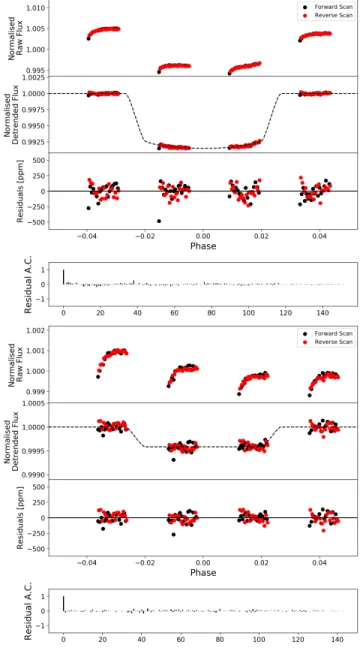
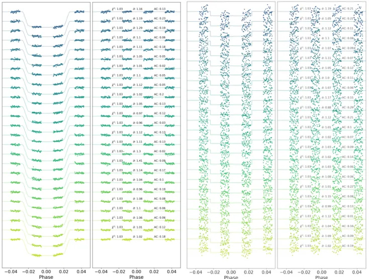
Morello et al. 2020). Figure1shows the raw white light-curve, the detrended white light-light-curve, and the fitting residuals for both observations while Figure2shows the fits of spectral light-curves for each wavelength.
2.3. Atmospheric characterisation - TauREx3 The reduced spectra obtained using Iraclis were there-after fitted using TauREx3 (Al-Refaie et al. 2019), a publicly available2 Bayesian retrieval framework. For the star parameters and the planet mass, we used the values from Bieryla et al. (2015) listed in Table 2. In our runs we assumed that KELT-7 b possesses a pri-mary atmosphere with a ratio H2/He = 0.17. For the opacity sources, we used the line lists from the ExoMol
2https://github.com/ucl-exoplanets/TauREx3_public
Figure 1. White light-curve for transmission (top) and emission (bottom) observations of KELT-7 b. For each panel; Top: raw light-curve, after normalisation. Second: light-curve, divided by the best fit model for the systematics. Third: residuals. Bottom: auto-correlation function of the residuals.
project (Tennyson et al. 2016), along with those from HITRAN and HITEMP (Rothman et al. 1987; Roth-man et al. 2010). In this publication, we considered six trace gases: H2O (Polyansky et al. 2018), CO(Li et al.
2015), TiO (McKemmish et al. 2019), VO (McKemmish et al. 2016), FeH (Dulick et al. 2003;Wende et al. 2010) and H- (John 1988; Edwards et al. 2020a). For H-, the absorption depends only on the mixing ratios of neu-tral hydrogen atoms and free elections. As this is a degenerate problem, we fixed the neutral hydrogen vol-ume mixing ratio and imposed a profile inspired from
4
Figure 2. Spectral light-curve fits from Iraclis of transmission (left) and emission (bright) spectra - for clarity, an offset has been applied. In each plot, the left segment shows the spectral light-curves while the residuals are shown in the right section. χ is the reduced chi squared, σ is the ratio between the standard deviation of the residuals and the photon noise, and AC is the auto-correlation of the fitting residuals.
Parmentier et al.(2018) using the two-layer model from
Changeat et al.(2019). The only remaining free param-eter is log(e-). Clouds are modelled assuming a fully opaque grey opacity model.
In this study we use the plane-parallel approximation to model the atmospheres, with pressures ranging from 10−2to 106Pa, uniformly sampled in log-space with 100 atmospheric layers. We included the Rayleigh scatter-ing and the collision induced absorption (CIA) of H2– H2 and H2–He (Abel et al. 2011; Fletcher et al. 2018;
Abel et al. 2012). Constant molecular abundance pro-files were used, and allowed to vary freely between 10−12 and 10−1 in volume mixing ratio. For the transit spec-tra, the planetary radius, which here corresponds to the radius at 10 bar, was allowed to vary between ±50% of the literature value. In emission, we set the planet ra-dius to the best-fit value from our transmission retrieval.
The cloud top pressure prior ranged from 10−2 to 106 Pa, in log-uniform scale. For the day side, we do not consider clouds in the model. In transmission, the temperature-pressure profile was assumed to be isother-mal while in emission a 3-point profile was used.
Finally, we use Multinest (Feroz & Hobson 2008;Feroz et al. 2009a,2013) with 1500 live points and an evidence tolerance of 0.5 in order to explore the likelihood space of atmospheric parameters.
2.4. Modelling Equilibrium Chemistry - petitCODE To help contextualize our free retrieval results, we computed a self-consistent forward model with petit-CODE, a 1D pressure-temperature iterator solving for radiative-convective and chemical equilibrium (Molli`ere et al. 2015, 2017). The code includes opacities for H2, H−, H
2O, CO, CO2, CH4, HCN, H2S, NH3, OH, C2H2, PH3, SiO, FeH, Na, K, Fe, Fe+, Mg, Mg+, TiO and
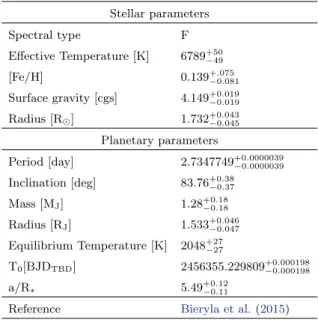
Stellar parameters Spectral type F Effective Temperature [K] 6789+50−49 [Fe/H] 0.139+.075−0.081 Surface gravity [cgs] 4.149+0.019−0.019 Radius [R ] 1.732+0.043−0.045 Planetary parameters Period [day] 2.7347749+0.0000039−0.0000039 Inclination [deg] 83.76+0.38−0.37 Mass [MJ] 1.28+0.18−0.18 Radius [RJ] 1.533+0.046−0.047 Equilibrium Temperature [K] 2048+27−27 T0[BJDTBD] 2456355.229809+0.000198−0.000198 a/R∗ 5.49+0.12−0.11
Reference Bieryla et al.(2015)
Table 1. Target parameters used in this study.
VO, as well as radiative scattering and collision induced absorption by H2–H2and H2–He. The atmosphere com-puted with petitCODE is assumed to be cloud-free, but the possibility of condensing refractory species is in-cluded in the equilibrium chemistry. Our petitCODE model for KELT-7 b was computed using the stellar and planetary parameters determined by Bieryla et al.
(2015). Here, the surface gravity was computed using the planetary mass and radius. Furthermore, an in-trinsic temperature of 600K was adopted, in accordance with its high equilibrium temperature (Thorngren et al. 2019). Finally, a global planetary averaged redistribu-tion of the irradiaredistribu-tion was assumed.
2.5. Ephemeris Refinement
Accurate knowledge of exoplanet transit times is fun-damental for atmospheric studies. To ensure the KELT-7 b can be observed in the future, we used our HST white light curve mid time, along with data from TESS (Ricker et al. 2014), to update the ephemeris of the planet. TESS data is publicly available through the MAST archive and we use the pipeline from Edwards et al. (2020b) to download, clean and fit the 2 minute cadence data. KELT-7 b had been studied in Sector 19 and after excluding bad data, we recovered 9 transits. These were fitted individually with the planet-to-star radius ratio (Rp/Rs) and transit mid time (Tmid) as free parameters. We note that the ephemeris of KELT-7 b was also recently refined by Garhart et al. (2020) and we also used the mid times derived in that study.
3. RESULTS
Our analysis uncovers a rich transmission spectrum which is consistent with a cloud-free atmosphere and suggests the presence of water and dissociated hydro-gen, as shown by the posterior distributions in Figure
3. We calculate the Atmospheric Detectability Index (ADI) Tsiaras et al. (2018) to be 16.8 for the trans-mission spectrum, indicating strong evidence of atmo-spheric features. The retrieved temperature of around 1400 K for the terminator region is consistent with the expected value given the equilibrium temperature. How-ever, as we are in temperature regime (Teq ' 2000 K) where 3D effects across the limb could occur, we may be biased on the abundances and temperature retrieved (Pluriel et al. 2020).
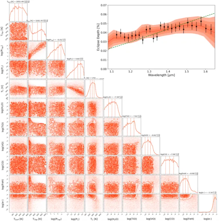
In contrast, the extracted emission spectrum does not contain strong absorption or emission features. Al-though the data is not consistent with a simple black-body, as shown in Figure 4, it can be explained by a varying temperature-pressure profile and H-. We cal-culate the ADI against a simple blackbody to be 19.6, highlighting the poorness of the blackbody fit and indi-cating the presence of a detectable atmosphere. How-ever, it could also indicate that 2D effects, such as those suggested by (Wilkins et al. 2014), are affecting the served spectrum. In their study of CoRoT-2 b they ob-served an emission spectrum similar to that of KELT-7 b (i.e. one that is poorly fit by a blackbody but which can be better fit using 2 blackbodies). Such inhomo-geneities will certainly be important in the analysis of emission data from future missions (Taylor et al. 2020). Our best fit favours a thermal inversion in the strato-sphere of KELT-7 b. Although the lower part of the at-mosphere has large temperature uncertainties (between 1000 K and 3000 K), the middle and top temperature-pressure points are well-constrained enough to indicate a thermal inversion with a temperature at the top between 2900 K and 3700 K as shown in Figure 5. Both trans-mission and etrans-mission spectra, along with their best-fit solutions are shown in Figures3 and4.
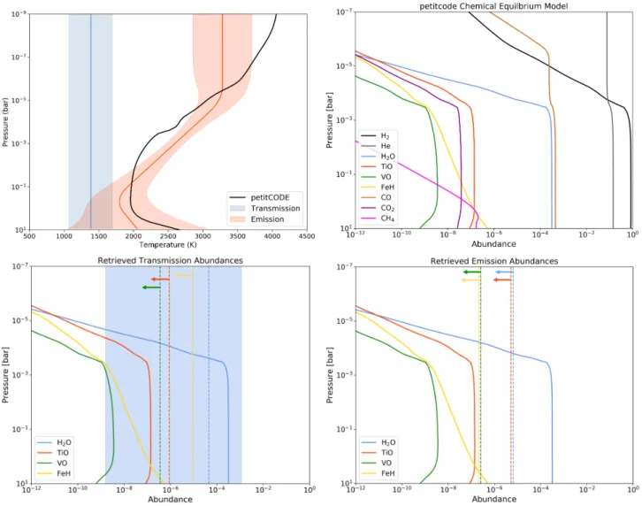
The retrieved emission temperature-pressure profile closely agrees with the petitCODE simulations, both showing a temperature inversion as shown in Figure5. The retrieved water abundance in transmission is consis-tent with the predictions although the 1σ upper bound in emission is below what is expected. For TiO, VO and FeH, the upper bound place on their abundances is significantly above the amount expected from our pe-titCODE simulations, suggesting the HST WFC3 data is no sensitive enough for us to conclude on their pres-ence/absence.
The transits of KELT-7 b from HST and TESS were seen to arrive early compared to the predictions from
6
Figure 3. KELT-7 b atmospheric retrieval posterior distributions of the transmission spectrum and the best-fit model with 3σ confidence in blue while the HST WFC3 data is represented by the black data points.
Bieryla et al. (2015). As the observation did not in-clude ingress or egress, the HST transit fitting is not as precise, and potentially not as accurate, as the TESS data which captured the whole event. Using this new data, we determined the ephemeris of KELT-7 b to be P = 2.KELT-734KELT-76541±0.00000036 days and T0 = 2458384.425577±0.000099 BJDT DB where P is the planet’s period, T0is the reference mid-time of the tran-sit and BJDT DB is the barycentric Julian date in the barycentric dynamical. Our derived period is 0.84 s and 0.063 s shorter than the periods fromBieryla et al.
(2015) andGarhart et al.(2020) respectively. The ∼10 minute residual of the TESS transits from the ephemeris of Bieryla et al.(2015) show the necessity to regularly follow-up transiting planets and for programmes such as ExoClock3 to which our observations have been
up-loaded. By the launch of Ariel in late 2028, around 1400 orbits of KELT-7 b will have occurred since the T0 derived here and the difference in the predicted transit
Figure 4. KELT-7 b atmospheric retrieval posterior distributions of the emission spectrum and the best fit retrieved with 3σ confidence in red while the HST WFC3 data is represented by the black data points. Also shown is a blackbody fit (green) which converged to a temperature of TBB ' 2500 K and does not well describe the observations.
times between the ephemeris from this work and from
Garhart et al.(2020) would be around 5 minutes. The observed minus calculated residuals, along with the fit-ted TESS light-curves are shown in Figure 6 while the fitted mid times can be found in Table3.
4. DISCUSSION
In transmission, H2O and H−, (log(H2O) = −4.34+1.41−4.45 and log(H−) = −4.26+1.41
−2.42) are well defined. As shown in the posterior distributions in Figure 3, correlations
exist between the abundances of the molecules, particu-larly between H2O and H−. We could expect to also find CO in such a hot atmosphere (Teq ' 2000K), evidence for which has been seen for other hot Jupiters: WASP-121b (Evans et al. 2017; Parmentier et al. 2018) and WASP-33b (Haynes et al. 2015). However our retrieval analysis on HST data only provides no evidence for the presence of these molecules. We also explored the
ad-8
Figure 5. Results of our self-consistent petitCODE model for KELT-7 b and our retrievals on WFC3 data. Top left: comparison of the temperature-pressure profiles. The petitCODE model (black) features a thermal inversion at 1 mbar, because of absorption by TiO and VO, and closely matches the retrieved profile. Top right: Molecular abundances for the petitCODE simulation. The equilibrium fractions of most molecules remain approximately constant for pressures higher than 1 mbar, but drop quickly at lower atmospheric pressures due to thermal dissociation. Bottom left: Comparison of constrained molecular abundances in transmission (dotted lines) to those from the petitCODE simulation (solid lines). The water abundance is seen to be within 1σ of that which is predicted. Bottom right: Comparison of upper bounds placed on molecular abundances in emission to those from the petitCODE simulation. The 1-σ upper bound on the water abundance is significantly lower than the petitCODE simulations. In both transmission and emission, the 1-σ upper bounds on TiO, VO and FeH are well above the predicted abundances, suggesting the data is not sufficient to comment on their presence/absence.
dition of Spitzer/IRAC and TESS data, see Section4.1
for more details.
The non-detection of TiO and VO in the termina-tor region agreed with predictions from Spiegel et al.
(2009). Their work suggests that in highly irradiated atmospheres, similar to KELT-7 b, TiO and VO would be likely to rain out in cold traps and disappear from the visible atmosphere. Observational evidence for these processes was reported in emission spectrum of Kepler-13Ab Beatty et al. (2017). To overcome these effects, large advective mixing and higher temperatures (higher than 1800K) would be required, leading to large
abun-dance of VO in the day side of the planet. However, in our analysis, we do not find evidence for VO or TiO on the day side of KELT-7 b, which could be unravelled with higher signal-to-noise in future observations such as Ariel or JWST. Also, our analysis potentially finds a large difference in the day/night temperatures with thermal inversion on the dayside, which would indicate that day and night side of the planet are poorly coupled by large scale dynamical processes, thus preventing VO and TiO from reaching the cold night side and conden-sating. Fortney et al. (2008) postulated that the pres-ence of optical absorbers would lead, and require, large
Retrieved parameters Bounds Transmission Emission log[H2O] -12 - -1 −4.34+1.41−4.45 < −5 log[e−] -12 - -1 −4.26+1.41 −2.42 < −5 log[F eH] -12 - -1 < −5 < −5 log[T iO] -12 - -1 < −5 < −5 log[V O] -12 - -1 < −5 < −5 log[CO] -12 - -1 < −5 < −5 µ (derived) - 2.33+0.28 −0.02 2.31 +0.22 −0.00 Rp(Rjup) ± 50% 1.47+0.02−0.02 -log Pclouds -2 - 6 3.91+1.31−1.56 -Tp[K] 1000-4000 1385+311−295 -Tbot p [K] 1000-4000 - 2053 +1145 −1164 Tmid p [K] 1000-4000 - 1710 +422 −474 Ttop p [K] 1000-4000 - 3282+463−573 ADI - 16.8 19.6 σ-level - > 5σ > 5σ Updated Ephemeris Period [days] 2.73476541±0.00000036 T0[BJDT DB] 2458384.425577±0.000099
Table 2. Table of fitted parameters for the retrievals of KELT-7 b transmission and emission spectra for HST data only and the updated ephemeris for the planet.
Epoch Transit Mid Time [BJDT DB] Reference
-742 2456355.229809 ± 0.000198 Bieryla et al.(2015) -232 2457749.959530 ± 0.000160 Garhart et al.(2020) -229 2457758.164460 ± 0.000190 Garhart et al.(2020) -124 2458045.316888 ± 0.000627 This Work* 158 2458816.518025 ± 0.000282 This Work 159 2458819.253548 ± 0.000220 This Work 160 2458821.987982 ± 0.000202 This Work 161 2458824.723075 ± 0.000183 This Work 162 2458827.457521 ± 0.000214 This Work 163 2458830.192334 ± 0.000196 This Work 164 2458832.927100 ± 0.000212 This Work 165 2458835.661872 ± 0.000246 This Work 166 2458838.396646 ± 0.000194 This Work
*Data from Hubble
Table 3. Transit mid times used to refine the ephemeris of planets from this study. All mid times reported in this work are from TESS unless otherwise stated.
day - night temperature contrasts, which could suggest that TiO and VO are present but simply beyond the sensitivity of the data.
4.1. Addition of Spitzer data
KELT-7 b has also been studied, in both transmission and emission, by the Spitzer Space Telescope using the each of the 3.6 µm and 4.5 µm channels of the InfraRed
Figure 6. Top: TESS observations of KELT-7 b presented in this work. Left: detrended data and best-fit model. Right: residuals from fitting. Bottom: Observed minus calculated (O-C) mid-transit times for KELT-7 b. Transit mid time measurements from this work are shown in gold (HST) and blue (TESS), while the literature T0 value is in red. The
black line denotes the new ephemeris of this work with the dashed lines showing the associated 1σ uncertainties and the black plot data point indicating the updated T0. For
com-parison, the previous literature ephemeris and their 1σ un-certainties are given in red. The inset figure shows a zoomed plot which highlights the precision of the TESS mid time fits.
Array Camera (IRAC). Combining data from multiple instruments or observatories has become the standard within the field as a way of increasing the spectral cov-erage, seeking to break the degeneracies that occur when fitting data over a narrow wavelength range (e.g. Sing et al. 2016). However, such a procedure is fraught with risk due to potential incompatibilities between datasets. Firstly, it has been shown using different orbital param-eters (a/Rs and i) in the fitting of the data can lead to offsets between the datasets (Yip et al. 2019). Secondly, the choice of limb darkening coefficients can cause verti-cal shifts in the spectrum (Tsiaras et al. 2018). Thirdly,
10
stellar variability, activity or spots can also induce off-sets in the recovered spectra (e.g. Bruno et al. 2020). Finally, imperfect correction of instrument systemat-ics can alter the fitted white light curve depth, again generating shifts between datasets, making the derived transit/eclipse depths incompatible (e.g.Stevenson et al. 2014b,a; Diamond-Lowe et al. 2014). Each of these ef-fects can of course affect HST data alone but, in this case, the offset would likely only lead to slight changes in the retrieved temperature or radius. When combining datasets, for instance HST WFC3 and Spitzer IRAC, off-sets in one of these, or differing offoff-sets in both, could lead to wrongly recovered abundances. In transmission and emission, Spitzer observations are sensitive to CH4 in the 3.6µm band and CO or CO2in the 4.5µm band while WFC3 data cannot constrain these molecules. Thus the detection, or non-detection, would be based entirely off the two Spitzer bands relative to the WFC3 data. An offset in either one of these would instigate the incor-rect recovery of the CH4, CO and CO2 abundances. In emission, these Spitzer points have been used as evi-dence for the presence of, or lack of, a thermal inver-sion. Differences in the correction of systematics have led to discrepant results (e.g. HD 209458 b: Knutson et al.(2008);Diamond-Lowe et al.(2014)).
Here, we tentatively add the Spitzer data for KELT-7 b, taken from the study by Garhart et al. (2020) of 36 hot Jupiters. For the fitting of the Spitzer eclipses,
Garhart et al. (2020) froze the orbital parameters to those from Bieryla et al. (2015), overcoming the first hurdle about combining datasets. The transit observa-tions were also fitted with fixed orbital parameters and limb darkening coefficients from Claret (2000), again showing consistency with our data. The latter two is-sues, of stellar variability or activity and the detrend-ing of instrument systematics, cannot be easily deter-mined without an overlap in spectral coverage. There-fore, we caution the reader that the compatibility of the datasets cannot be guaranteed. Additionally, we cau-tiously added the TESS data which was again fitted with same orbital parameters and limb darkening laws.
The best-fit retrieved spectra, both with and with-out the Spitzer data, is shown in Figure 7. Little dif-ference is seen between the fits, particularly in trans-mission where the best-fits are almost constantly within 1σ of each other. The recovered temperature pressure profiles are also practically identical. While this may suggest the data is compatible, it also shows that the information content of adding Spitzer, in this case, is rel-atively low. Therefore this begs the question of whether risking data incompatibility is worthwhile when there is little to gain. Figure 8 and 9 show posteriors from
the fittings with and without Spitzer, again highlight-ing the similarity between the fits. In transmission the only noticeable difference is in the recovered CO abun-dance, which is not constrained in the case of HST alone but the addition of Spitzer suggests an abundance of log(CO) = −4.56+1.72−4.69. The second change is in the water abundance recovered in emission, with HST and Spitzer converging to log(H2O) = −5.11+1.37−4.03 while no constraint can be made in the HST only case.
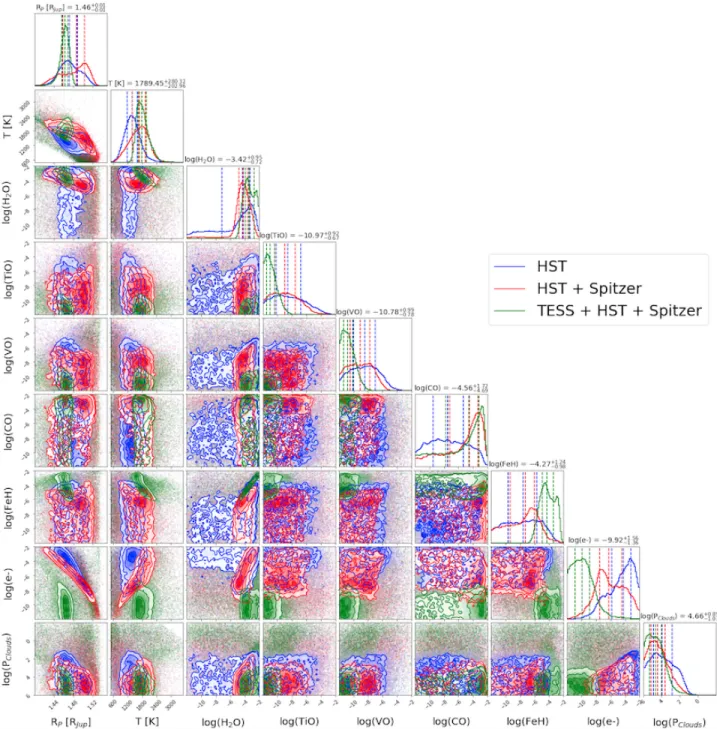
On the other hand, the addition of the TESS trans-mission data drastically changes the solution, remov-ing the detection of dissociated hydrogen, instead pre-ferring FeH to explain the absorption at the shorter wavelengths within the G141 grism due to the shallow TESS transit depth. We also explored the retrieved at-mospheric abundances in transmission without the H-opacity, again finding that there is little difference when adding Spitzer data as shown in Figure10. In this case, all data combinations readily agree on the abundances of H2O, FeH and CO. However, differences in seen in the evidence for TiO and VO, the presence of which the addition TESS data of rules out for log(TiO,VO) > -10, and in the recovered radius and terminator temper-ature, with the TESS dataset preferring a lower radius and higher temperature. We suggest it is imperative to, at the very least, study multi-instrument data sets sep-arately, as well as combined, when doing model fitting, as we have done in this study.
4.2. Future Characterisation
The most effective solution to understanding the source of the absorption seen in transmission between 1.1-1.3 µm would be to take more data, namely with the G102 grism of WFC3 which covers 0.8-1.1 µm. As there is also archival STIS transmission data for KELT-7 b, with the G430L and GKELT-750L grisms, this would provide continuous coverage from 0.3-1.6 µm, allowing for better constraints on the abundances of these opti-cal absorbers. We would also advocate for additional eclipse observations with WFC3, with either grism, to increase the spectral coverage and/or increase the sig-nal to noise, which may allow for spectral features to be uncovered.
Additionally, future space telescopes JWST (Greene et al. 2016), Twinkle (Edwards et al. 2018) and Ariel (Tinetti et al. 2018) will provide a far wider wavelength range and these missions will definitively move the ex-oplanet field from an era of detection into one of char-acterisation, allowing for the identification of the molec-ular species present and their chemical profile, insights into the atmospheric temperature profile and the detec-tion and characterisadetec-tion of clouds. Ariel, the ESA M4
Figure 7. Best-fit spectra (left) and temperature-pressure profiles (right), with one sigma errors in each case, for transit (top and middle) and eclipse (bottom) observations of KELT-7 b with HST data only, HST and Spitzer (red) and HST, Spitzer and TESS (green). The top transmission plots, and the emission case, include the H- opacity while the middle plots do not.
mission due for launch in 2028, will conduct a survey of ∼1000 planets to answer the question: how chemi-cally diverse are the atmospheres of exoplanets? KELT-7 b has been identified as an excellent target for study with Ariel (Edwards et al. 2019), through both trans-mission and etrans-mission spectroscopy, and simulated error bars fromMugnai et al.(submitted) have been added to the best-fit spectra to showcase this. Figure 11 shows simulated Ariel and JWST observations and highlights the wavelength coverage performed by those future mis-sions. Additionally ExoWebb (Edwards et al. 2020) has been used to showcase the capability of JWST for study-ing this planet.
5. CONCLUSION
We present spectroscopic transmission and emission observations of KELT-7 b taken with Hubble WFC3. While the transit spectra demonstrates strong absorp-tion features indicative of H2O and H−, the emission spectrum lacks features and can be fitted with CIA alone. We also explore adding data from Spitzer IRAC, with the results being very similar in both transmission and emission. Finally, we find that adding TESS data in our analysis strongly modifies our results. As these instruments do not provide spectral overlap, more data is needed to fully understand the source of the optical absorption seen in transmission. Further observations with Hubble, or with the next generation of observato-ries, will undoubtedly allow for an enhanced probing of the atmosphere of this intriguing planet. The analysis of
12
archival Hubble data is an essential preparatory step in enriching our comprehension of exoplanet atmospheres, allowing us to begin to appreciate their true diversity and understand the optimal observation strategy for upcoming facilities.
Acknowledgements: This work was realised as part of ARES, the Ariel Retrieval Exoplanet School, in Biar-ritz in 2019. The school was organised by Jean-Philippe Beaulieu, Angelos Tsiaras and Ingo Waldmann with the financial support of CNES.
This work is based upon observations with the NASA/ESA Hubble Space Telescope, obtained at the Space Telescope Science Institute (STScI) operated by AURA, Inc. The publicly available HST observations presented here were taken as part of proposal 14767, led by David Sing (Sing 2016). These were obtained from the Hubble Archive which is part of the Mikulski Archive for Space Telescopes. This paper includes data collected by the TESS mission which is funded by the NASA Explorer Program. TESS data is also publicly available via the Mikulski Archive for Space Telescopes (MAST). We are thankful to those who operate this archive, the public nature of which increases scientific productivity and accessibility (Peek et al. 2019). This work is also based in part on observations made with the Spitzer Space Telescope, which is operated by the Jet Propulsion Laboratory, California Institute of Tech-nology, under a contract with NASA. Finally, we thank our anonymous referee for suggesting we include the
Spitzer data which, along with other useful comments, led to the improvement of the manuscript.
JPB acknowledges the support of the University of Tasmania through the UTAS Foundation and the en-dowed Warren Chair in Astronomy, Rodolphe Cledas-sou, Pascale Danto and Michel Viso (CNES). BE, QC, MM, AT and IW are funded through the ERC Starter Grant ExoAI (GA 758892) and the STFC grants ST/P000282/1, ST/P002153/1, ST/S002634/1 and ST/T001836/1. NS acknowledges the support of the IRIS-OCAV, PSL. MP acknowledges support by the European Research Council under Grant Agree-ment ATMO 757858 and by the CNES. RB is a Ph.D. fellow of the Research Foundation–Flanders (FWO). WP and TZ have received funding from the Euro-pean Research Council (ERC) under the EuroEuro-pean Union’s Horizon 2020 research and innovation pro-gramme (grant agreement no. 679030/WHIPLASH). OV thanks the CNRS/INSU Programme National de Plan´etologie (PNP) and CNES for funding support. GG acknowledges the financial support of the 2017 PhD fellowship programme of INAF. LVM and DMG acknowledge the financial support of the ARIEL ASI grant n. 2018-22-HH.0.
Software: Iraclis (Tsiaras et al. 2016b), TauREx3 (Al-Refaie et al. 2019), pylightcurve (Tsiaras et al. 2016a), ExoTETHyS (Morello et al. 2020), ArielRad (Mugnai et al. submitted), ExoWebb (Edwards et al. 2020), Astropy (Astropy Collaboration et al. 2018), h5py (Collette 2013), emcee (Foreman-Mackey et al. 2013), Matplotlib (Hunter 2007), Multinest (Feroz et al. 2009b), Pandas (McKinney 2011), Numpy (Oliphant 2006), SciPy (Virtanen et al. 2020).
APPENDIX
TauREx3 employs Bayesian statistics as the cornerstone for the retrieval analysis (Waldmann et al. 2015a,b). Bayes’ theorem states that:
P (θ | x, M) = P (x | θ, M) P (θ, M)
P (x | M) (1)
where P (θ, M) is the Bayesian prior, M is the forward model. P (θ | x, M) is the posterior probability of the model parameters θ given the data, x assuming the forward model M. Bayesian analysis is implemented in TauREx3 via nested sampling (NS).
TauREx3 includes the implementation of NS Bayesian statistics via Multinest (Feroz & Hobson 2008;Feroz et al. 2009a,2013). NS employs Monte Carlo approach which constrains via ellipsoids encompassing the parameter space of the highest likelihood. NS determines the Bayesian evidence which is given by:
E = Z
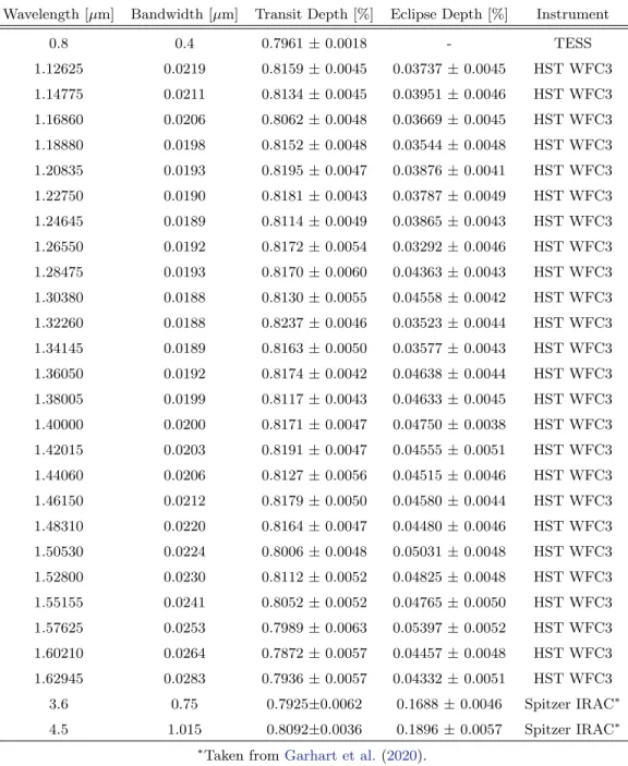
Wavelength [µm] Bandwidth [µm] Transit Depth [%] Eclipse Depth [%] Instrument 0.8 0.4 0.7961 ± 0.0018 - TESS 1.12625 0.0219 0.8159 ± 0.0045 0.03737 ± 0.0045 HST WFC3 1.14775 0.0211 0.8134 ± 0.0045 0.03951 ± 0.0046 HST WFC3 1.16860 0.0206 0.8062 ± 0.0048 0.03669 ± 0.0045 HST WFC3 1.18880 0.0198 0.8152 ± 0.0048 0.03544 ± 0.0048 HST WFC3 1.20835 0.0193 0.8195 ± 0.0047 0.03876 ± 0.0041 HST WFC3 1.22750 0.0190 0.8181 ± 0.0043 0.03787 ± 0.0049 HST WFC3 1.24645 0.0189 0.8114 ± 0.0049 0.03865 ± 0.0043 HST WFC3 1.26550 0.0192 0.8172 ± 0.0054 0.03292 ± 0.0046 HST WFC3 1.28475 0.0193 0.8170 ± 0.0060 0.04363 ± 0.0043 HST WFC3 1.30380 0.0188 0.8130 ± 0.0055 0.04558 ± 0.0042 HST WFC3 1.32260 0.0188 0.8237 ± 0.0046 0.03523 ± 0.0044 HST WFC3 1.34145 0.0189 0.8163 ± 0.0050 0.03577 ± 0.0043 HST WFC3 1.36050 0.0192 0.8174 ± 0.0042 0.04638 ± 0.0044 HST WFC3 1.38005 0.0199 0.8117 ± 0.0043 0.04633 ± 0.0045 HST WFC3 1.40000 0.0200 0.8171 ± 0.0047 0.04750 ± 0.0038 HST WFC3 1.42015 0.0203 0.8191 ± 0.0047 0.04555 ± 0.0051 HST WFC3 1.44060 0.0206 0.8127 ± 0.0056 0.04515 ± 0.0046 HST WFC3 1.46150 0.0212 0.8179 ± 0.0050 0.04580 ± 0.0044 HST WFC3 1.48310 0.0220 0.8164 ± 0.0047 0.04480 ± 0.0046 HST WFC3 1.50530 0.0224 0.8006 ± 0.0048 0.05031 ± 0.0048 HST WFC3 1.52800 0.0230 0.8112 ± 0.0052 0.04825 ± 0.0048 HST WFC3 1.55155 0.0241 0.8052 ± 0.0052 0.04765 ± 0.0050 HST WFC3 1.57625 0.0253 0.7989 ± 0.0063 0.05397 ± 0.0052 HST WFC3 1.60210 0.0264 0.7872 ± 0.0057 0.04457 ± 0.0048 HST WFC3 1.62945 0.0283 0.7936 ± 0.0057 0.04332 ± 0.0051 HST WFC3 3.6 0.75 0.7925±0.0062 0.1688 ± 0.0046 Spitzer IRAC∗ 4.5 1.015 0.8092±0.0036 0.1896 ± 0.0057 Spitzer IRAC∗ ∗
Taken fromGarhart et al.(2020).
Table 4. Spectral data of KELT-7 b used in this study.
where P (x, M) is the evidence. These statistical products produced by Multinest are used to perform the best fit model selection. NS performed by Multinest also allows for efficient parallelisation which permits the usage of high performance cluster computing.
14
Figure 8. Posterior distributions for atmospheric retrievals of KELT-7 b with various datasets. The addition of Spitzer data brings little change to the atmospheric properties while TESS data drives the retrieval to favour FeH over H-. We note that this FeH abundance is far above the expected (log(FeH)∼ −7). The reported values for each parameter are those obtained with the fit on all three datasets.
Figure 9. Posterior distributions for atmospheric retrievals of the emission spectra of KELT-7 b with and without Spitzer data (blue and red respectively). The addition of Spitzer data brings little change to the atmospheric properties except the derived water abundance which appears clearly with Spitzer data. The reported values for each parameter are those obtained with the fit on both datasets.
16
Figure 10. Posterior distributions for atmospheric retrievals of the transmission spectra of KELT-7 b with various datasets, this time without including H- as an opacity source. The addition of Spitzer data again has little effect on the retrieved atmospheric properties while TESS data drives the retrieval to higher temperatures and rules out the presence of TiO and VO. All cases require an FeH abundance which is far greater than expected. The reported values for each parameter are those obtained with the fit on all three datasets.
Figure 11. Simulated Ariel and JWST observations of the best-fit solutions retrieved in this work. The top panels show transmission spectra while the bottom panels show emission spectra. For Ariel, 2 stacked observations have been assumed while for JWST we modelled a single observation with NIRISS GR700XD as well as an observation with NIRSpec G395M.
REFERENCES
Abel, M., Frommhold, L., Li, X., & Hunt, K. L. 2011, The Journal of Physical Chemistry A, 115, 6805
—. 2012, The Journal of chemical physics, 136, 044319 Al-Refaie, A. F., Changeat, Q., Waldmann, I. P., & Tinetti,
G. 2019, in prep
Astropy Collaboration, Price-Whelan, A. M., Sip˝ocz, B. M., et al. 2018,AJ, 156, 123
Beatty, T. G., Madhusudhan, N., Tsiaras, A., et al. 2017,
AJ, 154, 158
Bieryla, A., Collins, K., Beatty, T. G., et al. 2015,The Astronomical Journal, 150, 12
Bruno, G., Lewis, N. K., Alam, M. K., et al. 2020,
MNRAS, 491, 5361
Changeat, Q., Edwards, B., Waldmann, I. P., & Tinetti, G. 2019, arXiv e-prints, arXiv:1903.11180
Claret, A. 2000, A&A, 363, 1081
Collette, A. 2013, Python and HDF5 (O’Reilly)
Deming, D., Wilkins, A., McCullough, P., et al. 2013,ApJ, 774, 95
Diamond-Lowe, H., Stevenson, K. B., Bean, J. L., Line, M. R., & Fortney, J. J. 2014,ApJ, 796, 66
Dulick, M., Bauschlicher, C. W., J., Burrows, A., et al. 2003,ApJ, 594, 651
Edwards, B., Al-Refaie, A., Lagage, P., & Gastaud, R. 2020, in prep
Edwards, B., Mugnai, L., Tinetti, G., Pascale, E., & Sarkar, S. 2019,AJ, 157, 242
Edwards, B., Rice, M., Zingales, T., et al. 2018,
Experimental Astronomy, 47, 2963
Edwards, B., Changeat, Q., Baeyens, R., et al. 2020a,AJ, 160, 8
Edwards, B., Changeat, Q., Yip, K. H., et al. 2020b,
MNRAS,arXiv:2005.01684 [astro-ph.EP]
Espinoza, N., & Jord´an, A. 2015,MNRAS, 450, 1879
Evans, T. M., Sing, D. K., & Kataria, T. e. a. 2017,Nature, 548, 58
Feroz, F., & Hobson, M. P. 2008,MNRAS, 384, 449
Feroz, F., Hobson, M. P., & Bridges, M. 2009a,MNRAS, 398, 1601
—. 2009b,MNRAS, 398, 1601
Feroz, F., Hobson, M. P., Cameron, E., & Pettitt, A. N. 2013, arXiv e-prints, arXiv:1306.2144
Fletcher, L. N., Gustafsson, M., & Orton, G. S. 2018, The Astrophysical Journal Supplement Series, 235, 24 Foreman-Mackey, D., Hogg, D. W., Lang, D., & Goodman,
18
Fortney, J. J., Lodders, K., Marley, M. S., & Freedman, R. S. 2008,ApJ, 678, 1419
Garhart, E., Deming, D., Mandell, A., et al. 2020,AJ, 159, 137
Greene, T. P., Line, M. R., Montero, C., et al. 2016,ApJ, 817, 17
Haynes, K., Mandell, A. M., Madhusudhan, N., Deming, D., & Knutson, H. 2015,ApJ, 806, 146
Hoeijmakers, H. J., Ehrenreich, D., Kitzmann, D., et al. 2019,A&A, 627, A165
Hunter, J. D. 2007,Computing in Science & Engineering, 9, 90
John, T. L. 1988, A&A, 193, 189
Knutson, H. A., Charbonneau, D., Allen, L. E., Burrows, A., & Megeath, S. T. 2008,ApJ, 673, 526
Kreidberg, L., Line, M. R., Parmentier, V., et al. 2018,The Astronomical Journal, 156, 17
Kurucz, R. L. 1970, SAO Special Report, 309
Li, G., Gordon, I. E., Rothman, L. S., et al. 2015, The Astrophysical Journal Supplement Series, 216, 15 MacDonald, R. J., & Madhusudhan, N. 2017,MNRAS, 469,
1979
Madhusudhan, N., Knutson, H., Fortney, J. J., & Barman, T. 2014,Protostars and Planets VI
Martioli, E., Col´on, K. D., Angerhausen, D., et al. 2018,
MNRAS, 474, 4264
McKemmish, L. K., Masseron, T., Hoeijmakers, H. J., et al. 2019,Monthly Notices of the Royal Astronomical Society, 488, 2836
McKemmish, L. K., Yurchenko, S. N., & Tennyson, J. 2016,
MNRAS, 463, 771
McKinney, W. 2011, Python for High Performance and Scientific Computing, 14
Mikal-Evans, T., Sing, D. K., Goyal, J. M., et al. 2019,
Monthly Notices of the Royal Astronomical Society, 488, 22222234
Molli`ere, P., van Boekel, R., Bouwman, J., et al. 2017,
A&A, 600, A10
Molli`ere, P., van Boekel, R., Dullemond, C., Henning, T., & Mordasini, C. 2015,ApJ, 813, 47
Morello, G., Claret, A., Martin-Lagarde, M., et al. 2020,
AJ, 159, 75
Mugnai, L. V., Pascale, E., Edwards, B., Papageorgiou, A., & Sarkar, S. submitted, Experimental Astronomy Oliphant, T. E. 2006, A guide to NumPy, Vol. 1 (Trelgol
Publishing USA)
Parmentier, V., Line, M. R., & Bean, J. L. e. a. 2018,A&A, 617, A110
Peek, J., Desai, V., White, R. L., et al. 2019, in BAAS, Vol. 51, 105
Pluriel, W., Zingales, T., & Leconte, J. e. a. 2020, A&A Polyansky, O. L., Kyuberis, A. A., Zobov, N. F., et al.
2018, Monthly Notices of the Royal Astronomical Society, 480, 2597
Ricker, G. R., Winn, J. N., Vanderspek, R., et al. 2014,in Proceedings of the SPIE, Vol. 9143, Space Telescopes and Instrumentation 2014: Optical, Infrared, and Millimeter Wave, 914320
Rothman, L. S., Gamache, R. R., Goldman, A., et al. 1987,
Appl. Opt., 26, 4058
Rothman, L. S., Gordon, I. E., Barber, R. J., et al. 2010,
JQSRT, 111, 2139
Sing, D. 2016, The Panchromatic Comparative Exoplanetary Treasury Program, HST Proposal
Sing, D. K., Fortney, J. J., Nikolov, N., et al. 2016,Nature, 529, 59
Skaf, N., Fabienne Bieger, M., Edwards, B., et al. 2020, arXiv e-prints, arXiv:2005.09615
Spiegel, D. S., Silverio, K., & Burrows, A. 2009,The Astrophysical Journal, 699, 14871500
Stevenson, K. B., Bean, J. L., Fabrycky, D., & Kreidberg, L. 2014a,The Astrophysical Journal, 796, 32
Stevenson, K. B., Bean, J. L., Seifahrt, A., et al. 2014b,
The Astronomical Journal, 147, 161
Swain, M. R., Vasisht, G., & Tinetti, G. 2008, arXiv e-prints, arXiv:0802.1030
Taylor, J., Parmentier, V., Irwin, P. G. J., et al. 2020,
MNRAS, 493, 4342
Tennyson, J., Yurchenko, S. N., Al-Refaie, A. F., et al. 2016,Journal of Molecular Spectroscopy, 327, 73
Thorngren, D., Gao, P., & Fortney, J. J. 2019,ApJL, 884, L6
Tinetti, G., Vidal-Madjar, A., Liang, M.-C., et al. 2007,
Nature, 448, 169
Tinetti, G., Drossart, P., Eccleston, P., et al. 2018,
Experimental Astronomy, 46, 135
Tsiaras, A., Waldmann, I., Rocchetto, M., et al. 2016a, ascl:1612.018
Tsiaras, A., Waldmann, I. P., Rocchetto, M., et al. 2016b,
ApJ, 832, 202
Tsiaras, A., Waldmann, I. P., Tinetti, G., Tennyson, J., & Yurchenko, S. N. 2019,Nature Astronomy, 451
Tsiaras, A., Waldmann, I. P., Zingales, T., et al. 2018,AJ, 155, 156
Virtanen, P., Gommers, R., Oliphant, T. E., et al. 2020,
Nature Methods, 17, 261
von Essen, C., Mallonn, M., Welbanks, L., et al. 2019,
A&A, 622, A71
Wakeford, H. R., Sing, D. K., Deming, D., et al. 2013,
Waldmann, I. P., Rocchetto, M., Tinetti, G., et al. 2015a,
ApJ, 813, 13
Waldmann, I. P., Tinetti, G., Rocchetto, M., et al. 2015b,
ApJ, 802, 107
Wende, S., Reiners, A., Seifahrt, A., & Bernath, P. F. 2010,
A&A, 523, A58
Wilkins, A. N., Deming, D., Madhusudhan, N., et al. 2014,
ApJ, 783, 113
Yip, K. H., Waldmann, I. P., Tsiaras, A., & Tinetti, G. 2019, arXiv e-prints, arXiv:1811.04686
Zhou, Y., Apai, D., Lew, B. W. P., & Schneider, G. 2017,