HAL Id: halshs-00002458
https://halshs.archives-ouvertes.fr/halshs-00002458
Submitted on 31 Jan 2006
HAL is a multi-disciplinary open access
archive for the deposit and dissemination of
sci-entific research documents, whether they are
pub-lished or not. The documents may come from
L’archive ouverte pluridisciplinaire HAL, est
destinée au dépôt et à la diffusion de documents
scientifiques de niveau recherche, publiés ou non,
émanant des établissements d’enseignement et de
Decision making under uncertainty and inertia
constraints: sectoral implications of the when flexibility
Franck Lecocq, Jean Charles Hourcade, Minh Ha-Duong
To cite this version:
Franck Lecocq, Jean Charles Hourcade, Minh Ha-Duong. Decision making under uncertainty and
inertia constraints: sectoral implications of the when flexibility. Energy Economics, Elsevier, 1998, 20
(4/5), pp.539-555. �10.1016/S0140-9883(98)00012-7�. �halshs-00002458�
Decision making under uncertainty
and inertia constraints:
sectoral implications
of the when flexibility
Franck Lecocq Jean-Charles Hourcade
Minh Ha-Duong
Decision making under uncertainty
and inertia constraints:
sectoral implications
of the when flexibility
Franck Lecocq
Jean-Charles Hourcade Minh Ha-Duong
Abstract
Current debates on mitigation emphasize the role of the inertia of the economic system. Our aim in this paper is to study in more depth how sectorally dif
-ferentiated inertia impacts on optimal CO2-emission abatement policies. Using
the STARTS model, we show that optimal abatement levels and costs differ sensibly among sectors. Differential inertia is the critical determinant of this trade-off, especially in the case of a 20-year delay in the action, or in an un-derestimation of the growth of the transportation sector. In particular, the bur-den of any additional abatement efforts falls on the most flexible sector, i.e. the industry. Debates on mitigation emphasize the role of inertia of the eco-nomic system. This paper aims at studying more in depth how sectorally dif-ferentiated inertia should influence, optimal CO2 emission abatement policies. Using a two-sector version of STARTS, we show that under perfect expecta-tions, optimal abatement profiles and associated costs differ sensibly between a flexible and a rigid sector (transportation).In a second step, we scrutinize the role of the uncertainty by testing the case of a 20-year delay of action and an underestimated growth of the transportation sector. We do this for three con-centration ceilings and we point out the magnitude of the burden which falls on the flexible sector. We derive some policy implications for the ranking of public policies and for incentive instruments to be set up at international level. © 1998 Elsevier Science B.V. All rights reserved.
Keywords
Introduction
The policy debate about the optimal timing of the abatement of GHG has been deeply influenced by the paper of Wigley et al. (1996) in Nature which sug-gests that an early departure from current GHG emission trends may not be the most efficient way to stay below a 550 ppm GHG concentration ceiling. A postponed abatement would indeed avoid a premature replacement of capital stock, take advantage of cheaper carbon free techniques in the future and, transferring a given amount of expenditures later in time, would result in lower discounted costs. Despite the warnings of the authors, this paper has of-ten been interpreted as a ‘no action’ policy message, even though it should have led to emphasize a logical distinction between action and abatement: be-cause of inertia, immediate action may be required in order to be able to abate more in the future.
Without refuting this ‘when flexibility’ argument, Ha Duong, Grubb and Hourcade (HGH) demonstrated in Nature that treating the 550 ppm target as stochastic instead of deterministic would result in sensibly higher abatement over the near term because of the interplay between uncertainty and inertia (Ha Duong et al. 1997). In a stochastic framework indeed, inertia has a Janus’ role: it raises both the costs of premature abatement and the costs of further accelerated abatement due to a tightening up of initial targets.
We will investigate in more depth this interplay by elucidating its sectoral di-mension. If inertia matters, then the heterogeneity of capital stocks should be seriously considered: cars, buildings, industrial plants, transportation infra-structures have life cycles ranging from a few years to more than one century. This distribution cannot but have serious policy implications.
To provide some insights on these issues, we will use a version of the STARTS model (Sectoral Trajectories with Adaptation and Response Turnover of Stocks) which considers two sectors, a flexible and a rigid one. The choice of a two-sector model derives from a compromise between analyt-ical transparency, the need of numeranalyt-ical control over the results and empiranalyt-ical realism in order to point out some implications of the heterogeneity of capital stocks
We shall first propose a taxonomy of the forms of inertia involved. Then, after a description of STARTS, we will present some numerical experiments
ad-dressing the three following issues: (1) how the ‘when flexibility’ should be sectorally distributed under perfect foresight; (2) on what sector will fall the burden in case of accelerated abatement following a delay of abatement; and (3) what are the implications of an ‘underestimation’ of the growth of the rigid sector.
I
Inertia and timing of abatement in a
stochastic framework: lessons from recent
debates
I.1
The interplay between uncertainty and inertia
It has been recognized for a long time that climate policies are built “in a sea of uncertainties” (Lave 1991). First, despite current progress in climate sci-ences, we are not likely to know in the near future at what concentration level “dangerous interference with the climate system” would occur, which is the objective set by the Framework Convention on Climate Change. Second, other uncertainties, endogenous to human behaviours, may influence the timing of action:
• sudden changes in public concern: past experience suggests that
envir-onmental issues follow political life cycles not only driven by scientific discoveries or symptomatic events, but also by casual mismanagement of information (the ‘mad cow’ crisis) or by the combination of political parameters (the Waldsterben crisis, Hourcade et al. 1992),
• trends in energy demand and technology: most of the baselines retained
in recent forecasting studies incorporate expectations of stable or stead-ily increasing energy prices over the following decades. But these are not fully supported by recent analysis of structural determinants of oil prices, which underlines in particular the drastic decrease of the cost of new discoveries (Fagan 1997).
But it is only because of the inertia of our economic system that uncertainty matters: without inertia, switching from one emission path to another would be costless. The nature of this interplay has been explored in HGH in response
to WRE:1 selecting the same discount rate and autonomous technical progress
coefficient as WRE, they confirm that the least cost abatement path towards a 550 ppm concentration target should be only 2% below the baseline emissions in 2020 if the target is certain; but this departure should jump up to 14% in case of an uncertainty on the optimal ceiling (equiprobably 450, 550 and 650 ppm) resolved only in 2020. In this stochastic framework indeed the decision-making problem is to balance between the costs of switching towards a tighter target in 2020 and those of too strict a pathway before 2020 if the ultimate tar-get proves to be 650 ppm.
Observing the costs of a 20year delay in action can easily highlight this prob -lem. These prove modest if the optimal target appears to be 550 ppm, but really significant for 450 ppm; consequently, the costs of switching to 450 ppm too late dominate the costs of too early abatement if the optimal target happens to be 650 ppm. Unsurprisingly, this effect is all the more important as the resolution of uncertainties comes later: the optimal departure jumps up to 20% if full information occurs in 2035. This effect is strongly correlated with the degree of inertia: doubling the degree of inertia results in an increase of the cost of delay from 14% to 35%. Conversely costs of delay become negli-gible for capital life duration below 10 years.
I.2
Determinants of inertia
Discussions between top-down and bottom-up analysis about the so-called ef-ficiency gap at the end-use energy level matter for setting short-term abate-ment targets but do not encompass the most critical mechanisms at work in the long run. Final energy demand is driven indeed not only by the efficiency of the end-use equipment but also by structural changes in the production sectors (just in time processes, share of energy intensive industries), in life styles and human settlements. In other words part of the dynamics is determined by para-meters beyond the energy sector and whose inertia may be far higher.
Jaccard (1997) portrays the great diversity of the involved capital stock by a three-level hierarchy of the decisions governing its dynamics. We will reph-rase his taxonomy in the following way.
1 Hourcade and Chapuis (1995) demonstrated with a simulation model why, in case of the need
for accelerated action, inertia may constitute an important cost multiplier. In an optimal control model Grubb et al;(1996) demonstrated why early abatements should be all the more important as inertia is supposedly high in the system.
• The end use equipment: the decision is made by private decision-makers (households, a division in a company). The turnover of capital stock ranges from a few years to two decades. At this stage the relative cost of delivering a given energy service is the key selection criteria (under the constraints of information gaps and other market imperfec-tions).
• The infrastructure equipment and industrial processes: this
encom-passes the buildings, the major transit modes, and industrial infrastruc-ture whose turnover is measured in decades. This level is largely gov-erned by centralized public and/or private decision-makers. Every de-cision involves an amount of capital whose order of magnitude is far higher than in the previous level. One major difficulty stems from the fact that, except in the very energy systems, energy costs play only a minor role in the decision compared, for instance, to strategic criteria in the industry or cost/speed ratio in the transportation sector.
• Land-use and urban planning: this level is driven both by infrastructure
decisions and by specific public policies. These policies can either be explicit, i.e. aimed at shaping urban forms or the distribution of the hu-man settlements, or implicit i.e. influencing land use and urban patterns through subsidies to mobility, or rules governing tenants and landlords relationships. Curving trends at this hierarchical level is then not just a problem of capital stock turnover.
Inertia in the economic systems results mainly from the interactions between these three levels. For example, the very architecture of the buildings ines the air conditioning requirements. More importantly, urban forms determ-ine not only the transportation needs but also the relative share of journeys made on foot, on bicycles, by rail or by private car. The attraction of activities around the proximity of infrastructures, the induced investment, the nature of skills and the amount of embedded interests generate dynamics which are hard to curve overnight.
Furthermore, inertia sums up to the time of penetration of technical
innova-tions,2 and the ‘lock-in’ processes (Arthur 1989) due to learning-by-doing,
economies of scale, informational increasing returns and positive network ex-ternalities to induce bifurcations. Beyond a critical point, market forces tend
2 Past experiences suggest indeed that new energy sources take about 50 years to penetrate from
1% to only 50% of their ultimate potential because of the time needed to remove market and in -stitutional barriers to the diffusion of innovations and the obstacles due to imperfect information and imperfect foresight.
indeed to reinforce the first choice instead of correcting it, in a self-fulfilling process (Hourcade 1993). At date ‘t’, there are still several possible market equilibria at ‘t + n’, and several possible ‘states of the world’ characterized by different technical contents. The bifurcation towards one or another depends
on the very decisions made at ‘t’ and on the expectations at that time.3 We can
easily imagine, in the transportation sector for example, two very different equilibria with relatively similar total costs but very different carbon contents: they cannot be discriminated today, but the costs of shifting from the adopted one to the other in the future might be huge, all the more that the transition period is short.
II
STARTS: a modeling framework to capture
heterogeneity and inertia of capital stocks
II.1
A tentative modeling response
to substantive issues
II.1.1
Forms and degrees of inertia
Available models in the energy field incorporate descriptions of the energy production system at a desegregation level that varies in function of the data, computational capabilities and the very objective of the model. They incorpor-ate data on costs and inertia, which, however controversial they are, permit reasonable numerical experiments. But this is not the case for the determinants of the final energy demand, which are as critical to understand the inertia of the entire system.
The problem we are confronting is that both the lack of harmonized data on the capital stock turnover at each of Jaccard’s hierarchical levels and the pro-fessional separation between specialists in each field make it very difficult to model in a reasonable way the dynamic interactions to be considered. For ex-ample, available energy models represent the penetration of efficient cars but
3 Since the development of the ‘sunspot theory’ (Azeriadis and Guesnerie 1986), the plurality of
equilibria induced by different sets of expectations leading to self-fulfilling processes has been pointed out in other fields of economics than the economics of technology.
not the links between the modal transportation structure and the transportation needs: current practice is to resort to exogenous hypothesis about these para-meters. The risk is obviously to derive some misleading conclusions: energy demand in the developing countries projected without considering the lack of transportation infrastructure, abatement policy scenarios where the abatement comes in part from lower trends in the demand for gasoline and where the cor-responding costs are not accounted for because they occur in the transporta-tion sector.
The key issue is then how to capture the driving forces behind inertia in tech-nical change, which are very different in nature, and to describe not only the energy sector but also the non-energetic determinants of the energy demand whose dynamics are far from being only driven by the energy prices. In STARTS, we capture only Jaccard’s two first hierarchical levels because the data and scientific information required to build a fully comprehensive model is unavailable. We rely on an aggregated treatment of inertia in order to study its role in comparison to other key parameters (e.g. discount rate or the date of resolution of the uncertainties). The role of Jaccard’s third level is represented only through different baselines. Compared with the compact stylization of DIAM, STARTS is an attempt at disentangle the many sources of inertia at work. At the same time, its simple two-sector construction enables policy
im-plications to be drawn out of it without loss of generality.4
II.1.2
Cost function: leap-frogging vs. accelerated turnover
There are various ways of treating inertia at an aggregated level. In UR-GENCE (Hourcade and Chapuis, 1995) inertia acts as a cost multiplier func-tion of the increase of the capital turnover. In Hammit et al. (1992), it is treated endogenously through logistic penetration curves of technical change. Toth et al. (1997) explore tolerable windows of emission trajectories, but
in-troduce an arbitrary upper bound of the reduction rate |dE/dt| / E ≤ 10%. DIAM
endogenizes inertia in such a form that permanent and adjustment costs are separable; the cost function is additive and the inertia in the system is defined
by the weight of adjustment costs on permanent costs.5 This allows for
repres-4 A new version of STARTS, currently under development, will include four sectors: energy
supply, which can be calibrated on results of existing energy models, transportation, habitat and industry. This representation will allow for clarifying the distinction between the various types of capital involved. It will also permit to represent the fact that elasticity to price of energy de -mand evolves very differently in the three main final de-mand sectors.
5 Dimensional analysis shows that D can be interpreted as the characteristic duration of the glob
-enting high transition costs even if the incremental costs of the carbon free techniques in the new stabilized path are null or even negative. In STARTS such a possibility is described through an explicit representation of the capital turnover and of the penetration of new techniques.
STARTS considers indeed that achieving a given emission reduction in a con-text of inertia imposes a trade-off between two parameters:
• the redirection of investment towards carbon saving techniques: at a
constant capital turnover rate, tighter emission reductions require to by-pass the ‘natural’ decarbonization trend and to ‘leap-frog’ towards ex-pensive techniques;
• the acceleration of the turnover of capital stock through scrapping some
capital vintages before the end of their economic life.
For example, an economy replacing 25% of its capital every decade will be obliged to adopt a zero emission technique (a solar plant for instance) if it is committed to cut 25% of its emissions over the following 10 years. Now would the cost of such a technique be very high, it might be cost-effective to replace one additional capital vintage to install two gas plants saving each 12.5% of previous emissions. The optimal trade-off requires the marginal sav-ing on the abatement costs to be equal to the costs of scrappsav-ing equipment prematurely.
In STARTS, ls capital vintages denoted Kits coexist in each sector s at each
period t.6 Capital built at period t in sector s is characterized with an emission
index per unit of capital εts. Emissions Ets are supposed to depend directly on
the existing capital stock that operates at its full capacity.7 There is no
possib-ility of lumpiness of capital such as in Disgusts and Mäler (1996) and the eco-nomy is assumed to follow a steady growth path.
Ets = Ki,tsεt−i,s (1)
The εts terms constitute the first set of control variables. They stand for
decar-bonization levels, while ….. stand for the baseline values
pret D as the exponential half life time of equipments, then D can be related to the annual depre -ciation rate of capital δ, by D = (ln 2) / δ and, for δ = 4%/yr, we find D = 20 years.
6 Vintages are counted backward, i.e. vintage 1 is the youngest (built at period t−1) and vintage ls
the oldest.
7 Emissions, consumption and costs are annual flows but the model is computed using 10-year
II.2
Overall Mathematical structure
STARTS8 is an optimal control model which minimizes the total utility loss of
reaching a given concentration ceiling in a two sector economy, each sector being characterized by different capital life duration and different perspectives for the penetration and ultimate performance of backstop technologies.
Difficulties arise in fully developed growth model (Lecocq and Hourcade, 1997) from the fact that these tend to abate by reducing investment rates: as emissions depend on the level of capital, reducing capital stock becomes a mitigation option. Such a response is economically justified in a first best world, but has little chance to be adopted in a real economy. In fact, the con-centration ceiling will be seen as a new exogenous constraint. It might be de-cided to face it either by keeping the consumption/total investment ratio con-stant with lower productive investment or by conserving the productive in-vestment constant with reduced consumption. The latter assumption will be made in the following numerical experiments.
Therefore, in STARTS, total capital is an exogenous parameter: it is assumed to grow at a constant rate. Nevertheless, the age distribution of capital vin-tages remains variable, and constitutes the second set of control variables: the model is allowed to overinvest compared to the baseline, but always replacing prematurely scrapped vintages in order to keep total amount of capital con-stant.
II.2.1
Objective function
STARTS uses a logarithmic utility function of consumption given at each
point in time by the difference between C0t, the annual consumption in the
baseline case and the abatement expenditures from both acceleration and leap
frogging. The optimization program is thus given by Eq. (2) below, where ρ
stands for the pure time preference: MaxA,ε e−ρ
t
(2)
8 The following model is the third version of STARTS (Sectoral Trajectories with Adaptation
and Response Turnover of Stocks) (Hourcade and Lecocq, 1996 and 1997) and the first to offer a representation of the age structure of the existing capital stock.
The acceleration variables Ait in Eq. (3) below stand for the accelerated capital renewal. Eq. (4) forces total capital stock to remain equal to its baseline value
K0ts.9
Ki+1,t+1,s = Kits− Aits for 1 ≤ i ≤ ls−1 (3)
ki,t+1,s = K0ts (4)
Parameter Ki+1,t+1,s stands for the investment at period t.10
II.2.2
Under a concentration constraint
Numerical experiments could be carried out within a cost-benefit analysis. But this would require to enter into discussion about both the ultimate damage level and the very shape of the damage function, which would blur the analys-is of the role of differential inertia among sectors. A cost-efficiency analysanalys-is circumvents this difficulty and is closer to the very framework of the Kyoto protocol.
The objective of the model is therefore to maximize utility under the
con-straint of not overshooting the concentration ceiling Mceiling:
Mt≤ Mceiling (∀ t) (5)
where atmospheric CO2 concentration Mt is given by Eq. (6) below.
Mt+1 = Mt + N (6)
EDt is an exogenously given parameter which stands for non-industrial CO2
emissions (principally deforestation). Parameters β, δ and Minf are calibrated to
reproduce concentration scenarios in the baseline (IPCC 1994).
II.2.3
Abatement costs
Additional costs of ‘leap frogging’ are technical costs of low-CO2 emitting
techniques. We approximate current data (IPCC 1996) through a quadratic function of the wedge between baseline and current carbon efficiency index:
Clft,s = Cmaxs Lts K1,t+1,s (7)
9 In a complete model, investment I becomes a variable and equation (3) becomes (3') K 1t+1 = It
where capital is now free to evolve out of the BAU track.
10 Note that, provided it is verified at period 1, Eq. (4) has a positive solution K
1,t+1,s at each
Parameter Cmaxs gives the incremental cost (per unit of capital) of a 100%
emission reduction at initial period. Lts stands for the decrease of this cost due
to autonomous technical change.11
Additional costs of acceleration come from two main sources: first from the
difference between planned investment (i.e. K0t+1,s− K0t,s) and realized
invest-ment (K1,t+1,s). Second, the economy withstands a penalty due to the premature
replacement of capital, which is equal to the residual value of this capital.
This value at year y ≤ 1 If r is the investment discount rate and l the capital life
duration, this value at year y ≤ ls is given approximately by e-y. Hence:
Caccts = (K1,t+1,s− (K0t+1,s− K0t,s)) + Aits e-iN (8)
III
Numerical experiments
III.1
Model calibration
We will consider a ‘rigid’ and a ‘flexible’ sector characterized by different life duration. Both encompass the capital stock driving the energy demand and the corresponding energy supply. The ‘rigid’ sector covers transportation infra-structures (roads, airports or railways), and the part of urban planning which shapes urban forms and transportation needs within cities. The ‘flexible’ sector covers housing and industry. This means evidently that, in the following nu-merical experiments the structure of the buildings will not be considered and that abatement will come solely from technical change in the end-use equip-ment. The reason for this gross classification is that we chose to place the
fo-11 We run STARTS without induced technical change specification in order to facilitate
compari-son with existing models (DICE, MERGE, DIAM...). This point is of importance for policy-making, but stands beyond the scope of this paper.
Moreover, firms commitment to develop R&D program depends on their anticipations of the fu-ture market conditions, and especially of the fufu-ture prices. Public policies play a great role in the formation and the stabilization of those anticipations. If everyone agrees on the existence of such phenomena, its scale and influence is indeed widely debated. Both their mathematical rep -resentation and the calibration of such relations prove highly difficult.
Therefore, the model we developed include an autonomous technical change representation. In-duced technical change is ignored, which leads to biased results towards less abatement scenar-ios. Furthermore, our model does not try to represent agents anticipations. In fact, as in DICE for instance, our model displays a centrally planned economy in which separate ‘agents’ do not appear. The question of the decentralization of the optimum must still be addressed, but is obvi-ously beyond the scope of this paper.
cus upon transportation and urban infrastructures which have a far longer life duration than any other kind of capital (buildings excepted) and, more import-antly, give rise to typical self-reinforcing loops which upgrade the inertia of the economic system.
III.1.1
Choice of the baseline scenario
In our baseline scenario, production is supposed to grow at a constant 2% rate in the future. Emissions are based on the IS92a scenario (IPCC, 1996). They are extended up to the model horizon (2200) by assuming a constant
decoup-ling between emissions and growth. CO2 emissions then start decreasing in
2150 with a maximum at 22 GtC/year. Non-fossil fuel emissions EDt also
de-rive from IS92a.
The distribution of emissions between sectors is based on sectoral IIASA
pro-jections (1995) for a baseline scenario very similar to IS92a.12 In these
projec-tions the share of the transportation sector in emissions rises from 25% today to 31% in 2100.
The repartition of capital between sectors is more difficult to assess. It stems from the fact that a redesign in transportation patterns would affect not only specific transportation infrastructures but also part of urban infrastructures that shape the former ones. In the absence of reliable data, we adopt the con-ventional figure that one third of private and public building investment are sensitive to transportation. Strict transportation investment in OECD countries being 5-7% while total private and public construction amount to 45%, we come down to a gross 20% figure for rigid sector share in total capital.
We treat transportation share in the existing capital stock as constant though its share in emissions change. This is a reasonable structural trend assumption. For each sector, capital stock in the baseline is supposed to grow at the same
rate as the economy. Conforming with the above assumptions, parameters ε0ts
are13 calibrated to obtain baseline emissions with baseline capital stocks for
each sector.
12 Baseline emissions in the IIASA study are generally more optimistic than IPCC IS scenarios.
However, we relied on their higher emission scenario (A2 scenario) whose emission levels are similar to IS92a ones.
13 Therefore, we do not study here the impact of different initial capital age structure on
abate-ment policies. As a matter of fact, a country which has invested very recently has a very new capital stock and therefore less possibilities to accelerate (at least acceleration penalty would be higher). This point is of high interest in a regional abatement policy study, which is beyond the scope of this paper.
III.1.2
Cost function parameterization
The cost function in Eq. (7) is calibrated in order to obtain an overall 1% dis -counted loss of consumption for a 550 ppm target. This equation depends on the cost of a hypothetical carbon-free technique (Cmax) to be used if a 100% abatement is requested at initial time. It is assumed to decrease over time
(with parameter Lt). Such a calibration is less easy in a two-sector model than
in an aggregated one because it requires finding the costs of two backstop technologies.
In the following numerical experiments, we assume that costs are higher in the rigid sector (transportation) than in the flexible one. As a matter of fact, pending on experts’ judgments, backstop technologies in the former will de-rive either from electricity or power cells, which require an additional trans-formation step between primary energy and end-use service, or from biofuels, whose total costs should include the possible feedbacks on land-use and food production and the costs of waste disposal. Finally, as each scenario runs within given assumptions about urban forms, the modal switch to water or
railways is assumed to be very capital intensive.14
For the same reasons we assume autonomous technical change to be faster in the flexible sector (1% every year) than in the rigid one (0.25%), as the latter depends on the former.
III.2
Optimal sectoral abatement trajectories and
sectoral profiles
In this subsection, we study the optimal response to a deterministic constraint
on atmospheric CO2 concentration. The considered ceilings are 450, 550 and
650 ppm (denoted C450, C550 and C650).
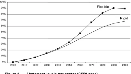
Fig. 1 displays the abatement levels in percent in each sector in the C550 case. Both curves are rather close until 2050, where abatement levels come to in-crease more rapidly in the flexible than in the rigid sector: in 2050, abatement levels are 30% and 33% in the rigid and flexible sectors, respectively, against
58% and 82% in 2080.15
14 In practice anyway, long standing policies may generate a set of urban forms and
transporta-tion patterns that, overall, do not cost more than the projected patterns. But in STARTS, this comes to design a new baseline scenario.
15 C450 and C650 cases display the same distribution of abatement levels, the only difference
0% 10% 20% 30% 40% 50% 60% 70% 80% 90% 100% 2000 2010 2020 2030 2040 2050 2060 2070 2080 2090 2100 Rigid Flexible
Figure 1 Abatement levels per sector (C550 case)
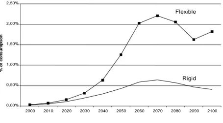
More important are the discrepancies between sectors in the abatement costs (Fig. 2) measured in consumption loss compared to baseline. These costs are comparable in the first periods (0.16% of consumption in 2020 in flexible against 0.11% in rigid) but diverge rather rapidly after 2020. The maximum of the wedge appears when both cost curves reach their peak value where 77% of the utility losses comes from the flexible sector.
The ‘peak’ shape of the time distribution of abatement costs is a direct con-sequence of the ‘law of motion’ of the model. Two contradictory sets of forces drive the optimal abatement path: autonomous technical change and discount-ing make it more interestdiscount-ing to abate later, while the irreversibility effect and the risk of an acceleration penalty push to early action. Most of the abatement expenditures are triggered when the abatement costs are dominated by the pos-sible penalty of accelerated abatement.
0,00% 0,50% 1,00% 1,50% 2,00% 2,50% 2000 2010 2020 2030 2040 2050 2060 2070 2080 2090 2100 % o f c o n s u m p ti o n Rigid Flexible
Figure 2 Abatement costs (C550 case)
Interestingly, within the numerical hypothesis of this experiment, the model never accelerates, even for a 450 ppm target. Intuitively, this result is due to the fact that an accelerated turnover comes to add a penalty to the cost of a given technique and the model logically selects a trajectory in order to avoid it. And if the abatement action starts now, it always finds a way to do this.
III.3
Differential impact of uncertainty
in a world with heterogeneous capital stock
What matters from a policy view point is how uncertainty may affect the cost distribution across sectors. This is why we analyze first the consequences of a 20-year delay in action and second the cost of an underestimation of the ex-pected growth of transportation needs.
III.3.1
Costs of a 20-year delay
In delayed response scenarios (D), mitigation policies are assumed to start only in 2020. Fig. 3 shows that the abatement levels in both sectors in the C550 and D550 cases do not to differ dramatically with and without delay. Confirming HGH results, abatement costs in the 550 C and D cases present no great difference (the total discounted loss in consumption rise from 1% to 1,03%). As to the abatement profile, the D curve stays below the C curve up to 2040 (flexible sector) and 2070 (rigid one) before passing over (with a max-imum of 12% in the flexible sector in 2060).
0% 10% 20% 30% 40% 50% 60% 70% 80% 90% 100% 2000 2010 2020 2030 2040 2050 2060 2070 2080 2090 2100
Rigid Flexible Rigid (Delayed) Flexible (Delayed)
Figure 3 Abatement levels with and without delays (C and D 550 cases)
This is only in the 450 ppm case (Fig. 4) that strong differences appear between C and D curves: the flexible sector takes the whole burden (100% abatement rate in 2040). The reason is that in this case, we reach a physical limit: achieving a 450 ppm target starting only in 2020 requires to increase the carbon annually saved by an additional 500 MtC each year between 2020 and 2040, which is twice the steepness of the C450 abatement profile.
0% 10% 20% 30% 40% 50% 60% 70% 80% 90% 100% 2000 2010 2020 2030 2040 2050 2060 2070 2080 2090 2100
Rigid Flexible Rigid (Delayed) Flexible (Delayed)
This highlights the non-linearity of the response to the value of the concentra-tion target. In the C450 and 550 cases, the model still had a wide margin of action to avoid acceleration while in the D cases, the margin is narrowed and inertia becomes critical. Thus the fact that in both D450 and D550 cases, the flexible sector bears a major part of the additional burden.
Note that the time distribution of the investment also reveals a propagation of the extra investment: the displacement of investment from period t + 1 to
peri-od t generates a new extra investment shock wave at periperi-od t + ls (at the end of
the life duration of the considered capital stock).
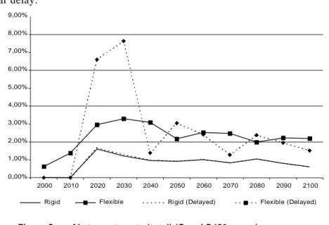
This evolution of the abatement profiles between C and D is mechanically translated in terms of costs (Fig. 5). Total discounted consumption loss rises significantly from 2.6% (C450 case) to 4.3% (D450 case), but the move of the peak of abatement costs is more impressive. In the C450 case, the ‘peak’ con-sumption loss in the flexible is 3% in 2030. In the D450 one, the ‘peak’ rises to 7.5% in 2020 and 2030, which obviously poses the question of the political realism of such a scenario. It is important to note that half that figure is gener-ated only by the cost of the accelergener-ated turnover, while in the 550 ppm case there is still a feasible path which do not require acceleration even with a 20-year delay. 0,00% 1,00% 2,00% 3,00% 4,00% 5,00% 6,00% 7,00% 8,00% 9,00% 2000 2010 2020 2030 2040 2050 2060 2070 2080 2090 2100
Rigid Flexible Rigid (Delayed) Flexible (Delayed)
Figure 5 Abatement costs (total) (C and D450 cases)
A second lesson of this exercise is to highlight how misleading it might be to rely only on aggregated measures. Run with one aggregated sector giving the same aggregated abatement profiles, STARTS calculates a 5% penalty in case
of delayed action. This aggregated figure masks more important sectoral shocks which may have important feedbacks on a real economy.
III.3.2
Costs of underestimating transportation growth
We assume in the T cases that the growth rate of the rigid sector is now 2.5% instead of 2% in the baseline scenario. This is a non-null probability hypo-thesis because of the uncertainties about growth of transportation sectors and urban forms in developing countries. According to IIASA (1995) projections, developing countries should indeed see their population rise by 60% and their per capita GDP more than triple by 2020. The induced needs for transportation services will be huge, and the correlative emissions will depend strongly on structural trends on the transportation modes and urban forms. Even though the increase of emissions is not very important (9% in 2100), this scenario is of interest as the global rigidity of the economy upgrades.
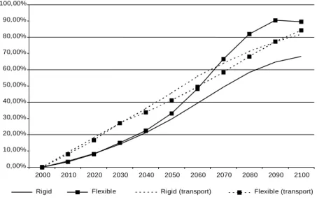
Fig. 6 compares the optimal abatement levels in the C and T cases for both sectors. The T curves differ strongly from the preceding ones: first the ment profiles of both sectors become rather parallel, second the optimal abate-ment levels appear more important in the T case over the short run. In 2020, abatement levels rise from 8% in the C550 curve to about 18% in the T ones.
0,00% 10,00% 20,00% 30,00% 40,00% 50,00% 60,00% 70,00% 80,00% 90,00% 100,00% 2000 2010 2020 2030 2040 2050 2060 2070 2080 2090 2100
Rigid Flexible Rigid (transport) Flexible (transport)
Figure 6 Abatement levels (C and T550 cases)
This can logically be explained by the fact that if trend in the rigid sector is proved to be higher, the margins of freedom in the flexible sector are not wide
enough to avoid the need of accelerated abatement in the rigid sector. Then an optimal strategy requires to act sooner in the rigid sector. Mathematically, when the share of the rigid sector is higher, the implicit value of marginal abatement in this sector increases as it prevents higher (acceleration) abate-ment costs in the future. To put it in another way, so as to avoid acceleration costs, the optimal trade-off between ‘rigid’ and ‘flexible’ abatement is dis-placed towards rigid ones in case of perfect foresight.
Unsurprisingly, the cost of a 20-year delay becomes more stringent. As in the D450 case, the delayed T450 case prove to be difficult to achieve: peak costs rise up to 21% of current consumption, and both flexible and rigid sectors now accelerate to withstand the shock. A 20-year delay in the T550 case does not result in any acceleration. But a significant difference compared with the D case is that the costs of delay, which were previously negligible (about 3% from C to D550 cases) tends out to be 30%.
The policy implication is that the expected magnitude of the rigid sector mat-ters critically for short term action.
Conclusion
Numerical exercises presented in this paper do not pretend to provide more than specific insights on the implications of the differential inertia in capital stocks. The qualitative results confirm intuition; optimally indeed the curving down of emission trends should start early in sectors characterised by a high inertia, and, in case of delayed action or of underassessment of the growth of these sectors, the burden falls on the flexible one. Less intuitive is the magnitude and non linearity of the entailed costs for this sector; because of the ir -reversibility effects on both cumulated emissions and technical trends, the shock on the non flexible sector is very quickly of some orders of magnitude higher than the costs of a response under assumption of perfect expectation. This has three major policy implications.
First, this emphasises the fact, already flowing logically from WRE and HGH papers that an aggregate abatement figure for a short-term period is by no means a good measure of the relevance of action and that a clear distinction should be made between abatement and action. A country which would meet short-term targets thanks to abatements in the industry or in the electrical
devices without curving current trends in the transportation would be em-barked in a very sub-optimal strategy.
Second the differentiation rules for targets beyond the 2008–2012 budget peri-od of the Kyoto protocol, or for negotiating the entry of developing countries into Annex 1 of the Climate Convention, should not be grounded solely on ag-gregated figures without considering the relative share of transportation sector and building in the emissions.
Third a trading system may not suffice in generating a cost effective abate-ment pathway. Under the context of carbon taxes, it has been extensively ar-gued that the price signals should be very high to curb significantly trends of transportation demand. The same mechanism will be at work in the setting of an emission trading. In the absence of accompanying structural measures in the urban planning or modal structures, it is then plausible that a low price of emission permits over a first period will not suffice in triggering a significant departure of current trends and that, in a second period, the price of permits increasing drastically, the industry will be forced to absorb the shock because of the inertia of capital stocks which will inhibit the capacity of the transport-ation or building sectors to react promptly.
In terms of research agenda, the implication is that further investigations are required to understand how trading systems may work in a context of hetero-geneous capital stocks and what are the necessary accompanying measures to account for the time lag between short term between price signals and technic-al adaptation in sectors where the energy costs are not the major driving force behind behaviours and policy choices.
Bibliography
C. W. Arthur, “Competing technologies, increasing returns and lock-in by his-torical trends”, Economic Journal, Vol 99, No 394, 1989, pp 116-131.
C. Azariadis, R. Guesnerie, “Sunspots and cycles”, Review of Economic
Stud-ies Vol 53, 1986, pp 725-737.
P. Dasgupta, K.-G. Mäler, Intergenerational Equity, Social Discount Rates
and Global Warming, communication to the EMF-RFF workshop Discounting
in Intergenerational DecisionMaking, Washington, november 14-15, 1996. M. N. Fagan, “Resource depletion and technical change: U.S. crude oil finding costs from 1977 to 1994”, Energy Journal, Vol.18, No 4, 1997, pp 91-105. M. Grubb, T. Chapuis, M. Ha Duong, “The economics of changing courses: implications of adaptability and inertia for climate policies”, Energy Policy, Vol 23, No 4/5, 1995, pp 417-432.
M. Ha Duong, M. Grubb, J.-C. Hourcade, “Influence of socio-economic iner-tia and uncertainty on optimal CO2-emission abatement”, Nature, Vol 390, 1997, pp 270-273.
J.K. Hammit, J.R. Lempert, M.E. Schlesinger, “A sequential decision strategy for abating climate change”, Nature, Vol 357, 1992, pp 315-318.
J.-C. Hourcade, T. Chapuis, “No regret potentials and technical innovation: a viability approach to integrated assessment of climate policies”, Energy
Policy, Vol 23, No 4/5, 1995, pp 433-445.
J.-C. Hourcade, “Modeling long-run scenarios: methodological lessons from a prospective study on a low CO2 intensive country”, Energy Policy, Vol 21, No 3, 1993, pp 309-324.
J.-C. Hourcade, J.-M. Salles, D. Thery, “Ecological economics and scientific controversies: lessons from some recent policy making in the EEC”,
Ecologic-al Economics, Vol 6, No 3, 1992, pp 211-233.
IIASA, Global energy perspectives to 2050 and beyond, WEC, London, 1995. IPCC, Climate Change 1995: Economic and Social Dimensions of Climate
Change (Bruce J., Lee H., Haites E. eds), Cambridge University Press,
IPCC Radiative forcing of climate change - Summary for policymakers, Cam-bridge University Press, CamCam-bridge, 1994.
M. Jaccard, Heterogeneous capital stock and decarbonating the atmosphere:
does delay make cents?, first draft, 1997.
Lave, “Formulating greenhouse policies in a sea of uncertainties”, Energy
Journal, Vol 12, No 1, 1991, pp 9-21.
F. Lecocq, J.-C. Hourcade, Timing of Climate Policies: the interplay between
valuing the future and beliefs in the damage curve shape, Communication to
the Integrated Assessment of Carbon Emissions workshop, IEW and EMF, II-ASA, Laxenburg, June 23-25, 1997.
F.L. Toth, T. Bruckner, H.-M. Füssel, M. Leimbach, G. Petschel-Held, The
tolerable windows approach to integrated assessment, communication at the
IPCC Asia Pacific Workshop on Integrated Assessment Models, Tokyo, Japan, march 10-12, 1997.
T.M.L. Wigley, R. Richels, J. Edmonds, “Economic and environmental choices in the stabilization of atmospheric CO2 concentrations”, Nature, Vol 379, 1996, pp 240-243.