The MIT Faculty has made this article openly available.
Please share
how this access benefits you. Your story matters.
Citation
Baker, Chris L., Rebecca Saxe, and Joshua B. Tenenbaum. “Action
understanding as inverse planning.” Cognition 113.3 (2009):
329-349.
As Published
http://dx.doi.org/10.1016/j.cognition.2009.07.005
Publisher
Elsevier
Version
Author's final manuscript
Citable link
http://hdl.handle.net/1721.1/60852
Terms of Use
Attribution-Noncommercial-Share Alike 3.0 Unported
Chris L. Baker, Joshua B. Tenenbaum & Rebecca R. Saxe
Department of Brain and Cognitive Sciences Massachusetts Institute of Technology
Abstract
Humans are adept at inferring the mental states underlying other agents’ actions, such as goals, beliefs, desires, emotions and other thoughts. We propose a computational framework based on Bayesian inverse planning for modeling human action understanding. The framework represents an in-tuitive theory of intentional agents’ behavior based on the principle of ra-tionality: the expectation that agents will plan approximately rationally to achieve their goals, given their beliefs about the world. The mental states that caused an agent’s behavior are inferred by inverting this model of ra-tional planning using Bayesian inference, integrating the likelihood of the observed actions with the prior over mental states. This approach formalizes in precise probabilistic terms the essence of previous qualitative approaches to action understanding based on an “intentional stance” (Dennett, 1987) or a “teleological stance” (Gergely et al., 1995). In three psychophysical experiments using animated stimuli of agents moving in simple mazes, we assess how well different inverse planning models based on different goal priors can predict human goal inferences. The results provide quantitative evidence for an approximately rational inference mechanism in human goal inference within our simplified stimulus paradigm, and for the flexible na-ture of goal representations that human observers can adopt. We discuss the implications of our experimental results for human action understanding in real-world contexts, and suggest how our framework might be extended to capture other kinds of mental state inferences, such as inferences about beliefs, or inferring whether an entity is an intentional agent.
Introduction
A woman is walking down the street, when suddenly she pauses, turns, and begins running in the opposite direction. Why? Is she just acting erratically on the way to her eventual goal? Did she change her mind about where she was going? Or did she complete an errand unknown to us (perhaps dropping off a letter in a mailbox) and rush off to her next goal? These inferences, despite their ordinariness, reveal a remarkable aspect of human cognition: our ability to infer the complex, richly-structured mental states that underlie others’ actions, given only sparse observations of their behavior.
Human social interaction depends on our ability to understand and predict other people’s actions in terms of the psychological states that produce behavior: chiefly, beliefs and desires. Much like visual perception, action understanding proceeds unconsciously and effortlessly but is the result of sophisticated computations that effectively solve an ill-posed, inductive problem, working backwards from sparse data to rich representations of the underlying causes. Our goal in this paper is to elucidate the computations involved in human action understanding through a combination of computational modeling and behavioral experiments. We will describe some of the first models that can explain how people perform these inferences so successfully, and that can also predict with surprising quantitative accuracy the judgments that people make.
Vision is often said to be a kind of “inverse graphics”, where graphics describes the causal physical process by which images are formed from scenes. Similarly, action under-standing can be characterized as a kind of “inverse planning” or “inverse reinforcement learning” (Ng & Russell, 2000). Just as computer graphics is based on mathematical mod-els of image formation, mathematical accounts of planning and reinforcement learning have been developed by economists, computer scientists, psychologists and neuroscientists (Bell-man, 1957; Watkins, 1989; Sutton & Barto, 1998; W. Schultz et al., 1997), which provide rational models of how agents should choose sequences of actions, given their goals, their prior experience, and their model of the world. Explaining an agent’s actions in terms of mental states requires inverting a model of its planning process, or inverse planning: working backwards to infer the desires and beliefs that caused the agent’s behavior.
Formalisms for solving the forward problems of planning and reinforcement learning are often divided into model-based and model-free approaches (Sutton & Barto, 1998; Doya, 1999; Daw et al., 2005), and there is evidence that the brain has systems corresponding to both (W. Schultz et al., 1997; Dickinson, 1985). We propose that the same kinds of cognitive machinery that support learning goal-directed action in the model-based approach – the ability to build models of the world and plan reward-maximizing sequences of actions over them – can be used in an inverse direction to infer the goals behind other agents’ observed behavior.
Philosophers and psychologists have long considered non-formal versions of this pro-posal in discussions about “belief-desire psychology”. Fig. 1(a) illustrates a typical example: a folk theory that specifies intentional agents’ beliefs and desires as the causes of their be-havior (c.f. Dennett, 1987; Wellman, 1990; Perner, 1991; Gopnik & Meltzoff, 1997). Dennett (1987) argues that this causal relation is governed by the principle of rationality: the ex-pectation that intentional agents will tend to choose actions that achieve their desires most efficiently, given their beliefs about the world. At a qualitative level, inverse planning is simply running the principle of rationality in reverse. Considered as a formal computation, however, inverse planning is significantly more difficult than forward planning. Just as in vision (Barrow & Tenenbaum, 1981; Richards et al., 1996), the inverse problem is ill-posed. Its solution requires strong prior knowledge of the structure and content of agents’ mental states, and the ability to search over and evaluate a potentially very large space of possible mental state interpretations. Implementing a formal version of this account, and quantita-tively evaluating it with human behavioral judgments is the main contribution of our work here.
(c) Perceptual Access Environment Belief Goal Action Principle of rational action Principle of rational belief (b) Environment Goal Action Principle of rational action (a) Belief Desire Action Principle of rational action Situations General World Knowledge General Preferences
Figure 1. Modeling intuitive theories of intentional action. Diagrams use causal graph notation. Shaded nodes represent observed variables; unshaded nodes represent latent variables whose values must be inferred. Dotted boxes indicate the causal relation between variables. In this example, the observations are an agent’s Action in some Environment and the agent’s Perceptual Access to the value of the Environment. Given this evidence, the agent’s Belief and Goal must be inferred. (a) Non-formal “belief-desire psychology” account of folk theories of intentional action. Non-formal accounts of human action understanding typically assume some version of this causal structure, and define the causal relation between beliefs, desires and actions in terms of qualitative, context-specific commonsense rules (e.g. Wellman & Bartsch, 1988; Fodor, 1992). (b) A simplified version of (a) proposed by Gergely et al. (1995) and Csibra & Gergely (1997) as a model of infants’ early-developing action understanding competency. We formalize this intuitive theory as Bayesian inverse planning. The functional form of the causal relation between Environment, Goal and Action is given by rational probabilistic planning in Markov decision problems, and goal inference is performed by Bayesian inversion of this model of planning. (c) A generalized framework for human action understanding. This relates the non-formal account in (a) to the formal model in (b) by sketching how agents’ Beliefs and Desires (or Goals) depend on their Perceptual Access to the Environment, mediated by their General World Knowledge and General Preferences. The model in (b) is a limiting case of (c), in which agents are assumed to have complete Perceptual Access to the Environment, constraining their Beliefsto be equal to the Environment.
of behavior are qualitatively consistent with the inverse planning view (Meltzoff, 1995; Gergely et al., 1995; Meltzoff, 1988; Gergely et al., 2002; Csibra et al., 2003; Sodian et al., 2004; Phillips & Wellman, 2005). Six-month-old infants interpret simple human motions as goal-directed actions, and expect that subsequent behavior will be consistent with these inferred goals (Woodward, 1998). That is, when actions could be interpreted as a rational or efficient means to achieve a concrete goal, infants expect the actor to continue to use the most efficient means to achieve the same goal, even when the environment changes. Gergely, Csibra and colleagues found that six- to twelve-month old infants extend the same expec-tations to the novel (and relatively impoverished) movements of two-dimensional shapes (Gergely et al., 1995; Csibra et al., 1999, 2003). In this context, infants’ inferences were
flexible and productive: given information about any two of the environment, the action and the goal, infants could infer the likely value of the third. To account for these findings, Gergely et al. (1995) proposed an early-developing, non-mentalistic version of Fig. 1(a), shown in Fig. 1(b). On their account, the Environment represents concrete situational con-straints on the agent’s available actions, such as the agent’s own location and the location of other agents, objects, or obstacles, and the Goal is some point or entity in the Environment. Together, the Environment and Goal provide a basis for the agent’s Action under a simple version of the rationality principle known as the teleological stance. Gergely et al. (1995) argue that this simplified schema forms the core of a more sophisticated, later-developing mentalistic theory of intentional action.
This research, along with the essential computational difficulty of action understand-ing, raises several open questions about how action understanding works in the mind. Can human action understanding competency be described by formal models, or is our intuitive psychological knowledge vague and heterogeneous? If action understanding can be formal-ized, can people’s judgments be explained by models of inverse planning? Does inverse planning explain people’s judgments better than simple heuristic alternatives? If human judgments are best explained by inverse planning, what is the form and content of our rep-resentations of agents’ mental states and actions – the priors that make inductive mental state inferences possible?
To address these questions, we formalize action understanding as a Bayesian inference problem. We model the intuitive causal relation between beliefs, goals and actions as rational probabilistic planning in Markov decision problems (MDPs), and invert this relation using Bayes’ rule to infer agents’ beliefs and goals from their actions. We test our framework with psychophysical experiments in a simple setting that allows us to collect a large amount of fine-grained human judgments to compare with the strong quantitative predictions of our models.
Specifically, we use the tools of Bayesian inverse planning to formalize the action understanding schema shown in Fig. 1(b). Inspired by Gergely et al. (1995), we assume that the agent’s Action depends directly on the Environment and the Goal, without requiring a separate representation of the agent’s beliefs. To specify the agent’s likely Actions as a function of the constraints of the Environment and the agent’s Goal, these variables are encoded within an MDP, and the causal relation between them is computed by a mechanism for rational planning in MDPs. We assume that the planning relation is probabilistic, tolerating a certain amount of noise or variability in how agents can execute their plans.
Fig. 1(c) sketches a more general intuitive theory of rational action, intended to capture various qualitative proposals in the theory of mind literature (e.g. Wellman & Bartsch (1988); Wellman (1990); Bartsch & Wellman (1995); see also Goodman et al. (2006) for a related formal account). This schema extends Fig. 1(a) by describing how beliefs depend on perceptual access to the environment, mediated by general world knowledge, and how goals depend on general preferences over states of the world. General world knowledge and preferences are high-level variables that apply across situations, while new beliefs and goals are generated specifically for each situation. The specific models we work with in this paper (Fig. 1(b)) correspond to the special case in which agents are assumed to have full perceptual access to the environment, thereby constraining the contents of their beliefs to be equal to the environment. A formal implementation of the more general framework in
Fig. 1(c) is beyond our scope here, but in the General Discussion we consider the additional computational assumptions needed to extend our work in that direction, to allow reasoning about the unknown contents and origins of agents’ beliefs.
The Bayesian inversion of MDP models of behavior requires strong priors over the space of agents’ goals. In our framework, the most basic concept of a goal corresponds to the objective to bring about a particular state of the environment. However, this is clearly too inflexible to describe the sophisticated kinds of goals that humans can attribute to other agents, and there are many ways that the basic goal concept can be extended. As a first step, in this paper we consider two extensions to the most basic goal concept, which roughly correspond to the explanations of the woman’s behavior in the introductory vignette: goals that can change over time and goals with more complex content, such as subgoals along the way to a final goal. We also formulate a simple heuristic alternative based on low-level motion cues as a limiting case of the changing-goal prior. We describe Bayesian inverse planning models based on these different goal priors in the Computational Framework section, and compare how accurately they predict people’s judgments in our experiments.
Our experiments use a stimulus paradigm of animated displays of agents moving in simple maze-like environments to reach goal objects, inspired by stimuli from many previous studies with children and adults (e.g. Heider & Simmel, 1944; Gergely et al., 1995; R. Gel-man et al., 1995; Scholl & Tremoulet, 2000; Tremoulet & FeldGel-man, 2000; Zacks, 2004; R. T. Schultz et al., 2003; J. Schultz et al., 2005; Tremoulet & Feldman, 2006). This paradigm allows fine-grained experimental control of agents’ actions, environment and plausible goals, and is ideal for both psychophysical experiments and computational modeling. Although this methodology greatly simplifies real-world action understanding, these kinds of stimuli evoke a strong sense of agency and the impression of mental states to adults (Heider & Simmel, 1944; Tremoulet & Feldman, 2000, 2006) (even when adult subjects are instructed not to make mentalistic interpretations (Heberlein & Adolphs, 2004)), and can lead to the formation of expectations consistent with goal-directed reasoning in infants (Gergely et al., 1995; Csibra et al., 1999, 2003). There is evidence that these kinds of stimuli recruit brain regions associated with action perception in adults (Castelli et al., 2000; R. T. Schultz et al., 2003; J. Schultz et al., 2005), suggesting a common mechanism with real-world action under-standing. Further, these stimuli can represent quite complex situations and events (Heider & Simmel, 1944), with similar abstract structure to more naturalistic contexts. Similarly, our computational models can be extended to much more general contexts than the simple scenarios in our experiments, as we will show with several examples in the Computational Framework section.
We present three experiments, which measure people’s online goal inferences, retro-spective goal inferences, and prediction of future actions based on previous goal inferences, respectively. Taken together, our experiments test whether human action understanding in our experimental domain can be explained by inverse planning. Individually, our ex-periments probe the space of representations that people apply in action understanding. Each experiment includes special conditions to distinguish the predictions of inverse plan-ning models based on different goal priors. By comparing which of these models produces inferences that match people’s judgments most accurately in each experimental context, we show how our approach can be used to elucidate the prior knowledge applied in human
action understanding.
Computational Framework
Our computational framework formalizes action understanding as Bayesian inverse planning: the Bayesian inversion of models of probabilistic planning in Markov decision problems (MDPs). This section will provide an overview of our framework and its appli-cation to our experimental stimuli. First, we will describe the encoding of the maze-world scenarios of our experiments into MDPs. We will also sketch the MDP encoding of several more realistic environments and contexts than those of our experiments to emphasize the generality of Bayesian inverse planning principles. Next, we will describe the computations underlying the mechanism for planning in MDPs. We will then sketch the Bayesian com-putations involved in inverting MDP models of planning, and give examples of the kinds of structured goal priors that are required to perform these computations. Finally, we will compare our framework with previous models of action understanding. Our overview in this section will be fairly high-level, with the formal details provided in a separate appendix.
Our framework uses MDPs to capture observers’ mental models of intentional agents’ goal- and environment-based planning. MDPs are a normative framework for modeling sequential decision making under uncertainty, widely used in rational models of human planning and reinforcement learning (Dayan & Daw, 2008), and in real-world applications in operations research and other fields (Feinberg & Shwartz, 2002; Puterman, 2005). An MDP represents an agent’s model of its interaction with its environment. MDPs encode all relevant information about the configuration of the world and the agent with the state variable. MDPs also represent the affordances of the environment: what actions the agent can take and a causal model of how these actions change the state of the world. Finally, MDPs represent the subjective rewards or costs caused by the agent’s actions in each state. In our maze-world scenarios, the state includes the location of all obstacles, potential goals and other objects, and the location of the agent. Agents can take 9 different actions: Stay, North, South, East, West, NorthEast, NorthWest, SouthEast and SouthWest, except when these actions are blocked by obstacles. For simplicity, we assume that actions always lead to their intended movements. The agent’s goal is to achieve a particular state of the world, and each action is assumed to produce a small cost to the agent until this goal is reached. Once the agent reaches its goal it is satisfied, and these costs cease. We define costs to be proportional to the negative distance of the intended movement: actions North, South, East, and West have costs proportional to −1, and actions NorthEast, NorthWest, SouthEast and SouthWest have costs proportional to −√2. We also define the cost of the Stay action to be proportional to −1 to capture the desire for continual progress toward the goal. Formally, these assumptions induce a class of stochastic shortest path problems (Bertsekas, 2001), implying that rational agents should plan to reach their goal as quickly and efficiently as possible.
To illustrate the application of MDPs to another domain, consider the game of golf. In golf, the state is comprised by the current hole, the current score, the current stroke number, and the position of the ball. Actions must specify club selection and the type of shot to be attempted. The causal model of the effect of actions reflects the inherent uncertainty about where a shot ends up, with the outcome of difficult shots being more uncertain than others. In golf, each shot has a cost of 1, and rational players try to minimize their score.
In addition to golf, many other games can be modeled as MDPs, such as blackjack (Sutton & Barto, 1998), backgammon (Tesauro, 1994), Tetris (Bertsekas & Tsitsiklis, 1996), and football (Bertsekas & Tsitsiklis, 1996).
As another example, consider the job of the head chef of a restaurant. Given a menu, the chef’s goal is to prepare each dish as well and as quickly as possible to maximize customer satisfaction and restaurant capacity. The state consists of the number of kitchen staff and the available ingredients, burners, ovens, cooking implements, counter space, et cetera. Actions include delegation of tasks to kitchen staff, the allocation of cooking resources to different dishes, and the chef’s own hands-on preparation of dishes. As in golf, the causal model reflects the uncertainty in preparation time and the performance of staff members. Relative to golf, cooking has rich logical and hierarchical structure, where every step has a large number of pre- and post-conditions, and individual actions may enable multiple subsequent steps. For instance, sending a line cook after two raw eggs furthers both the goal to cook a frittata as well the goal to prepare a souffl´e.
Planning formally describes the way that intentional agents choose actions to achieve their goals in an MDP. An optimal plan is one that provides the minimum-expected-cost course of action to the goal from every state. Our models assume that agents choose the optimal action only probabilistically. This yields a probability distribution over Actions, given a Goal and the Environment, denoted P (Actions|Goal, Environment), which provides the functional form of the probabilistic planning relation in Fig. 1(b). We assume that an agent’s actions are distributed in proportion to the softmax function of the expected value (negative expected cost) of each available action. The level of determinism in the agent’s actions is represented by the parameter β: higher β values yield greater determinism (less noise), and lower β values yield less determinism (more noise). We describe an algorithm for probabilistic planning based on dynamic programming (Bellman, 1957) in the appendix. Given an MDP model of goal-directed planning, Bayesian inverse planning computes the posterior probability of a Goal, conditioned on observed Actions and the Environment, using Bayes’ rule:
P(Goal|Actions, Environment) ∝ P (Actions|Goal, Environment)P (Goal|Environment). (1) In this equation, P (Actions|Goal, Environment) is the likelihood of the Goal given ob-served Actions and the Environment, defined above as probabilistic planning in an MDP. P(Goal|Environment) is the prior probability of the Goal given the Environment, which sets up a hypothesis space of goals that are realizable in the environment. Inverse planning integrates bottom-up information from observed actions and top-down constraints from the prior to infer the Goal, given observed Actions and the Environment. We describe inverse planning models based on several different goal priors below.
Inverse planning also enables goal-based prediction of future actions in novel situ-ations, given prior observations of behavior in similar situations. For simplicity, in this paper, our goal-based prediction experiment presents scenarios where agents’ environments and goals remain constant across observations (although our framework handles cases where the environment changes as well (Baker et al., 2006)). Action prediction averages over the probability of possible future Actions′, given a Goal and the Environment, weighted by the posterior over the Goal given previously observed Actions and the Environment from Equa-tion 1. This is just the posterior predictive distribuEqua-tion over future AcEqua-tions′ given previous
Actionsand the Environment:
P(Actions′|Actions, Environment) = X
Goal
P(Actions′|Goal, Environment)P (Goal|Actions, Environment). (2)
We use Equations 1 and 2 to model people’s judgments in our experimental tasks. In Experiment 1, we model people’s online goal inferences using an online version of Equation 1. In Experiment 2, we model people’s retrospective goal inferences using a smoothed version of Equation 1. In Experiment 3, we model people’s predictions of agents’ future actions, given observations of their past behavior of varying complexity, using Equation 2.
We formulate several inverse planning models, based on different forms of the prior over goals, which we refer to as M1, M2 and M3. Each model specifies a family of goal priors depending on one or a few continuous parameters. These models are surely much too simple to capture the full range of goals that people can attribute to an intentional agent, and they simplify in different ways. Each model should be thought of as just a first approximation to some aspects of people’s goal priors, embodying certain abstract principles that could be important (along with many others) in structuring our expectations about intentional action. By comparing the predictions of these models to people’s judgments from our experiments, we test the extent to which they capture significant dimensions of people’s prior knowledge, and in what contexts. We sketch the goal priors used by M1, M2 and M3 below. The formal details of these goal priors are provided in the appendix, including derivations of Equations 1 and 2 specific to each model.
The first inverse planning model we consider (M1) assumes that a goal refers to a single state of the environment that an agent pursues until it is achieved. Given a goal, probabilistic planning produces actions that tend to move the agent closer to the goal state, but depending on β, the level of determinism, planning can sometimes yield unexpected actions such as changes in direction or detours. Higher β values will fit actions that follow the shortest path very well, but will fit noisy action sequences very poorly. Lower β values will fit most action sequences moderately well, but will not fit any action sequence particularly closely. For example, in the introductory vignette the best explanation of the woman’s erratic behavior in terms of M1 is that she tends to pursue her goals in a particularly noisy manner, or has a low β value. Moreover, the assumption of a noisy (low β) agent is the only way that M1 can explain paths that deviate from the simplest notion of rational action, described by a shortest path to a single, fixed goal. Our other models also support such explanations; formally, they have the same β parameter representing the agent’s level of determinism. They differ in allowing a broader range of alternative explanations based on richer representations of agents’ possible goals.
The second inverse planning model we consider (M2) is an extension of M1 that assumes that agents’ goals can change over the course of an action sequence. This allows M2 to explain changes in direction or indirect paths to eventual goals, as in the attribution that the woman in the introductory vignette had changed her mind about where she was headed. M2 represents the prior probability that an agent will change its goal after an action with the parameter γ. With γ = 0, goal changing is prohibited, and M2 is equivalent to M1. With γ close to 0, the model rarely infers goal changes, implying that all past and
recent actions are weighted nearly equally in the model’s goal inferences. With γ close to 1, the model infers goal changes frequently, and only the most recent actions factor into the model’s goal inferences. Intermediate values of γ between 0 and 1 interpolate between these extremes, adaptively integrating or forgetting past information depending on the degree of evidence for subsequent goal changes.
The third inverse planning model we consider (M3) is an extension of M1 that assumes that agents can have subgoals along the way to their final goal. For example, M3 can capture the inference that the woman in the introductory vignette wanted to first complete a task (such as dropping off a letter) before pursuing her next goal. M3 represents the prior probability of a subgoal with the parameter κ. With κ = 0, subgoals are prohibited, and M3 is equivalent to M1. With κ > 0, M3 can infer a sequence of subgoals to explain more complex behaviors, such as paths with large detours from the shortest path to a final goal. Finally, we consider a simple alternative heuristic (H) based on low-level motion cues, inspired by Blythe et al. (1999), Zacks (2004) and Barrett et al. (2005). H looks only at an agent’s most recent action, rather than a whole sequence of actions, assuming that at any given time, the agent’s goal is probably the object toward which it had most recently moved. Including H in our comparisons allows us to test whether the full machinery of inverse planning is needed to explain human goal inferences, and in particular, the extent to which temporal integration over agents’ entire paths is an essential feature of these inferences. For the sake of comparison with our inverse planning models, we formulate H as a special case of M2 in which agents’ goals can change arbitrarily after every action, i.e. γ is set to its extreme value of 1. For many action sequences, both in our maze-world settings and in everyday situations, H makes similar predictions to the inverse planning models. These are cases that support a single unambiguous goal interpretation through the action sequence. However, our experiments are designed to include a subset of conditions with more complex trajectories that can distinguish between H and inverse planning models. Related Work
Previous computational models of action understanding differ from our framework along several dimensions. Much of the classic work on action understanding relies on logical representations of the domain and the agent’s planning process (Schank & Abelson, 1977; Kautz & Allen, 1986). These approaches use sophisticated, hierarchical representations of goals and subtasks, such as scripts and event hierarchies, to model the structure of agents’ behavior, and model goal inference in terms of logical sufficiency or necessity of the observed behavior for achieving a particular goal. Probabilistic versions of these ideas have also been proposed, which allow inductive, graded inferences of structured goals and plans from observations of behavior (Charniak & Goldman, 1991; Bui et al., 2002; Liao et al., 2004). However, these approaches assume that the distribution over actions, conditioned on goals, is either available a priori (Charniak & Goldman, 1991; Bui et al., 2002), or must be estimated from a large dataset of observed actions (Liao et al., 2004). An alternative is to model the abstract principles underlying intentional action, which can be used to generate action predictions in novel situations, without requiring a large dataset of prior observations. Various forms of the rationality assumption have been used to achieve this in both logical and probabilistic models of action understanding (Kautz & Allen, 1986; Ng & Russell, 2000; Verma & Rao, 2006). However, these models have not compared against human judgments,
and have not explored the kinds of structured goal representations necessary to explain human action understanding. In this paper, we integrate probabilistic models of rational planning with simple structured representations of agents’ goals to model human action understanding. Although we do not directly test any of the models described above, we test whether their computational principles can account for human goal inferences in our experiments.
Experiment 1
Our first experiment measured people’s online goal inferences in response to animated stimuli of agents moving to reach goal objects in simple maze-like environments. Our stimuli varied the environmental context, including the configuration of marked goals and obsta-cles, and varied agents’ paths and the point at which participants’ judgments were collected. This yielded fine-grained temporal measurements of human goal inferences and their sen-sitivity to various actions and contexts. We addressed the motivating questions from the Introduction by comparing how accurately M1, M2, M3 and H predicted participants’ judg-ments. Comparing models based on different goal priors revealed aspects of the form and content of the prior knowledge underlying human goal inferences. Comparing the accuracy of these models with H tested whether people’s judgments in our experimental domain were best explained as a process of inverse planning or the application of a simple heuristic. Method
Participants.
Participants were 16 members of the MIT subject pool, 9 female, 7 male. Stimuli.
Subjects viewed short animations of agents moving in simple mazes. Agents were represented by small moving circles, and as they moved through the environment, traces of their trajectories trailed behind them to record their entire movement history as a memory aid. Each displayed movement sequence paused at a judgment point: a point in the middle of the agent’s trajectory before a particular goal was achieved, where subjects reported their online goal inferences. The environment was a discrete grid of squares that agents could occupy, with dimensions of 17 squares wide by 9 squares high. Agents’ movements were restricted to adjacent squares, with directions {N,S,E,W,NE,NW,SE,SW}. Known goals were displayed as capital letters “A”, “B” and “C”, and walls were displayed as solid black barriers. Animations were shown from an overhead perspective (i.e. looking down on a room with a wall in the middle). Example stimuli from Experiment 1 are shown in Fig. 2(a).
Design.
All 36 conditions of Experiment 1 are shown in Fig. 3. Our experimental design varied three factors: goal configuration, obstacle shape and agent path. There were four different goal configurations, displayed in columns 1-4 of Fig. 3. Only the location of goal C changed across conditions; goals A and B were always in the upper and lower right corners, respectively. There were two different obstacle shapes: “Solid” and “Gap”. Every environment shown had a wall-like obstacle extending up from the bottom edge. In the
A B C A B C A B C A B C Experiment 1 Experiment 2 Judgment point: 7 Judgment point: 11 Judgment point: 7 Judgment point: 11 (a) (b)
Figure 2. Stimulus paradigm for Experiments 1 and 2. Each stimulus presented an animation of an agent’s path (marked by a dashed line) ending at a judgment point: a pause in the animation that allowed participants to report their online inferences of the agent’s goal at that point. (a) Experiment 1: online goal inference task. Subjects rated how likely each marked goal was at the judgment point. (b) Experiment 2: retrospective goal inference task. Subjects rated how likely each marked goal was at an earlier judgment point, given by the “+” along the dashed line.
Solid conditions this wall was unbroken, while in the Gap conditions it had a hole in the middle through which the agent could pass. The first, fourth, and seventh rows of Fig. 3 represent the Solid conditions, while the remaining rows represent the Gap conditions.
Based on the goal configuration and obstacle shape, the agent’s path was generated by making two choices: first, which goal (A, B or C) the agent was heading toward, and second, whether the agent went around the obstacle or through it. The second choice only applied in the Gap conditions; in the Solid conditions the agent could only move around the obstacle. In Fig. 3, paths are grouped as “A” paths, “B” paths and “C” paths, respectively. Because of C’s varying location, there were 8 unique C paths, while there were just two unique A paths and two unique B paths because the locations of A and B were fixed. All paths started from the same point, marked with an “x” in Fig. 3.
Each condition included a number of trials, which varied the length of the path shown before a judgment was required. Different conditions queried subjects at different judgment points, selected at informative points along the paths. Fig. 2(a) displays two stimuli with judgment points of 7 and 11, respectively, as they were plotted for our subjects. In Fig. 3, many of the initial trials are identical, and only differ in their eventual destination (e.g. corresponding trials in rows 1 and 4 of Fig. 3 are identical up to judgment point 10). Subjects were only shown unique stimuli, and after all redundant conditions were removed, there were 99 stimuli in total, all represented in Fig. 3.
Procedure.
Participants were given a cover story to establish assumptions about our experimental scenarios, including the assumption of intentional agency, a model of agents’ environments, and a hypothesis space of agents’ goals. Participants were told they would be viewing videos of members of an intelligent alien species collected by scientists, and that each video displayed a different alien moving toward a different goal in the environment. They were
Goal location 1 2 3 4 x -3 - - - 7 - - 10 11 -13 A B C x -3 - - - 7 - - 10 11 -13 A B C x -3 - - - 7 - - 10 11 -13 A B C x -3 - - - 7 - - 10 11 -13 A B C x 3 -7 - - 10 11 -13 A B C x 3 -7 - - 10 11 -13 A B C x 3 -7 - - 10 11 -13 A B C x 3 -7 - - 10 11 -13 A B C x 3 -7 - - 10 11 -13 A B C x 3 -7 - - 10 11 -13 A B C x 3 -7 - - 10 11 -13 A B C x 3 -7 - - 10 11 -13 A B C “A” paths x -3 - - - 7 - - 10 11 -13 A B C x -3 - - - 7 - - 10 11 -13 A B C x -3 - - - 7 - - 10 11 -13 A B C x -3 - - - 7 - - 10 11 -13 A B C x 3 -7 - - 10 11 -13 A B C x 3 -7 - - 10 11 -13 A B C x 3 -7 - - 10 11 -13 A B C x 3 -7 - - 10 11 -13 A B C x 3 -7 - - 10 11 -13 A B C x 3 -7 - - 10 11 -13 A B C x 3 -7 - - 10 11 -13 A B C x 3 -7 - - 10 11 -13 A B C “B” paths x -3 - - - 7 - - 10 11 -14 -16 A B C x -3 - - - 7 - - 10 11 -13 -15 A B C x -3 - - - 7 - - 10 11-- 14 A B C x -3 - - - 7 - - 10 A B C x -3 -7 A B C x 3 -7 8 A B C x 3 -7 - - 10 11 A B C x 3 -7 - - 10 11- 13 - 15 A B C x -3 -7 A B C x 3 -7 8 A B C x 3 -7 - - 10 11 A B C x 3 -7 - - 10 11- 13 - 15 A B C “C” paths “Solid” “Gap” (around) “Gap” (through) “Solid” “Gap” (around) “Gap” (through) “Solid” “Gap” (around) “Gap” (through)
Figure 3. All stimuli from Experiment 1. We varied three factors: goal configuration, obstacle shape and agent path. There were four goal configurations, displayed in columns 1-4. Path conditions are grouped as “A” paths, “B” paths and “C” paths. There were two obstacle shape conditions: “Solid” and “Gap”. There were 36 conditions, and 99 unique stimuli in total.
instructed that aliens could not pass through walls, but that they could pass through gaps in walls. They were told that after each video, they would rate which goal the alien was pursuing.
Stimulus trials were ordered with the earliest judgment points presented first to pre-vent hysteresis effects from showing longer trials before their shorter segments. Trials with the same judgment points were shown in random order. On each trial, the animation paused at a judgment point, allowing participants to report their online inferences of the agent’s goal at that point. Subjects first chose which goal they thought was most likely (or if two or more were equally likely, one of the most likely). After this choice, subjects were asked to rate the likelihood of the other goals relative to the most likely goal, on a 9-point scale from “Equally likely”, to “Half as likely”, to “Extremely unlikely”.
Modeling.
Model predictions take the form of probability distributions over agents’ goals, given by Equation 1 (specific versions for M1, M2, M3 and H are provided in the appendix). Our models assumed that all goals were visible, given by the three marked locations in our stim-uli. M3 assumed there were either 0 or 1 subgoals, which could correspond to any location in the environment. To put people’s goal inferences on the same scale as model predictions, subjects’ ratings were normalized to sum to 1 for each stimulus, then averaged across all subjects and renormalized to sum to 1. The within-subjects normalization guaranteed that all subjects’ ratings were given equal weighting in the normalized between-subjects average. Results
We present several analyses of how accurately M1, M2, M3 and H predicted people’s online goal inferences from Experiment 1. We begin with a qualitative analysis, which compares subjects’ data and model predictions from several conditions of Experiment 1 to illustrate the kinds of behavior that people are sensitive to in action understanding, and to show how closely inverse planning models captured people’s judgments. We then turn to several quantitative analyses which rigorously support our previous qualitative observations and address the motivating questions from the Introduction.
Fig. 4 shows examples of our qualitative comparisons between participants’ goal in-ferences and the predictions of M2. As we will argue quantitatively below, M2 was the model that best explained people’s judgments in Experiment 1. The conditions in Fig. 4(a) were selected to highlight the temporal dynamics of subjects’ ratings and model predictions in response to different observed actions and environments. Each condition in Fig. 4(a) differs from adjacent conditions by one stimulus feature, which illustrates the main effects of changing the goal configuration, the obstacle shape and the agent’s path.
Participants’ average ratings with standard error bars from these conditions are shown in Fig. 4(b). These examples illustrate several general patterns of reasoning predicted by our models. At the beginning of each trajectory, people tended to be uncertain about the agent’s goal. As more of the trajectory was observed, their judgments grew more confident (e.g. compare conditions 1 and 2 of Fig. 4(b)). A comparison of adjacent conditions in Fig. 4(b) shows how changing stimulus features had specific effects on people’s goal inferences – some subtle, others more dramatic.
x -3 -- -7- -1011 -13 A B C 3 7 10 11 13 0 0.5 1 3 7 10 11 13 0 0.5 1 3 -x -- -7- -1011 -13 A B C 3 7 10 11 13 0 0.5 1 3 7 10 11 13 0 0.5 1 3 7 10 11 13 0 0.5 1 3 7 10 11 13 0 0.5 1 11 -13 A B C 3 -x -- -7- -10 3 7 10 11 13 0 0.5 1 3 7 10 11 13 0 0.5 1 A B C 11 -13 3 -x -- -7- -10 3 7 10 11 13 0 0.5 1 3 7 10 11 13 0 0.5 1 A B C 1011 -13 x -3 - 7 -3 7 10 11 13 0 0.5 1 3 7 10 11 13 0 0.5 1 11-13 A B C 10 x -3 - 7 -(a) (b) (c) P(Goal|Actions) Model People Example conditions Average ratings A B C Judgment point Judgment point 1 Judgment point Judgment point 4 Judgment point Judgment point 2 Judgment point Judgment point 3 Judgment point Judgment point 5 Judgment point Judgment point 6
Figure 4. Example conditions, data and model predictions from Experiment 1. (a) Stimuli illus-trating a range of conditions from the experiment. Each condition differs from adjacent conditions by one feature—either the agent’s path, the obstacle, or the goal locations. (b) Average subject ratings with standard error bars for the above stimuli. (c) Predictions of inverse planning model M2 with parameters β = 2.0, γ = 0.25.
predicted people’s judgments with high accuracy across all conditions, including the effects of varying key stimulus features of the agent’s environment or path. M2 can be used to explain why participants’ judgments varied as they did across these conditions, based on the general expectations about rational action that M2 embodies: agents will tend to move along the most efficient paths toward their goal, and goals tend to stay constant over time but occasionally can change.
Conditions 1 and 2 in Fig. 4 differed only at the end of the path, after the agent had passed the obstacle. Before this point people assigned similar probabilities to goals A and B, because the trajectory observed was essentially the shortest path toward both goals. Beyond the obstacle the agent took a step in the direction of goal A (Condition 1) or goal B (Condition 2) and people’s uncertainty resolved, because the trajectory was now consistent with the shortest path to only one goal and departed significantly from the shortest path to the other.
Condition 3 in Fig. 4 differed from Condition 2 only in the presence of a gap in the obstacle. Relative to Condition 2, this resulted in a significantly lower probability assigned to goal B early on, as the agent went around the obstacle (see step 7 in particular). This can be thought of as a counterfactual inference: if the agent had been heading toward B originally, it would have gone straight through the gap rather than around the obstacle; this alternative shortcut path was not available in Condition 2. Once the agent had passed the obstacle and turned toward B, people were very quick to change their judgment to B. The model explained this as the inference that the agent’s goal, while initially probably A
or C, had now switched to B.
Condition 4 in Fig. 4 reversed the pattern of Condition 3: the agent initially went through (rather than around) the obstacle and then turned toward A (rather than B). Before the obstacle, people rated goal B most likely and A about half as likely, because the agent’s trajectory was along the shortest path to B and followed a less efficient path to A. Once the agent passed the obstacle and turned toward A, people changed their judgment to B, which the model explained as a change in the agent’s goal from B to A (or, less likely, the choice of an inefficient path to reach A).
Conditions 5 and 6 in Fig. 4 changed the position of C. Before the agent passed through the obstacle, the agent’s trajectory was now along the shortest path to B and C, which increased the relative probability assigned to C and decreased the probability of A and B. After the obstacle, the agent either turned toward A (Condition 5) or B (Condition 6). In Condition 5, this conflicted with previous evidence, and people quickly changed their goal inference to A, which the model explained as a change in goals (or the choice of a less efficient path). In Condition 6, the movement after the obstacle was consistent with B, the previously inferred goal, and the probability assigned to B continued to increase.
The basic logic of our quantitative analyses was to compare how accurately different models predicted people’s judgments using measures of correlation. Our overall quantitative analysis computed the correlation of each model class with people’s data and assessed the statistical significance of the differences between these correlations using bootstrap cross-validation (Cohen, 1995). Bootstrap cross-cross-validation (BSCV) is a technique for model selection, which measures the goodness-of-fit of models to data while preventing overfitting and controlling for model complexity. We describe the details of our BSCV analysis further in the appendix. The average correlations for each model from our analysis are shown in Table 1. M2 performed best, correlating significantly higher with people’s judgments than M1 (pBSCV <0.0001), M3 (pBSCV <0.0001) and H (pBSCV = 0.032). H performed second best, correlating significantly higher with people’s judgments than M1 (pBSCV < 0.0001) and M3 (pBSCV <0.0001). M3 correlated significantly higher with people’s judgments than M1 (pBSCV = 0.0004), and M1 performed worst.
M1 M2 M3 H
hri 0.82 (0.017) 0.97 (0.0046) 0.93 (0.012) 0.96 (0.0027)
Table 1: Bootstrap cross-validated correlation of inverse planning models and a simple heuristic alternative with people’s data from Experiment 1. Numbers in parentheses indicate standard devi-ation.
To illustrate the pattern of errors for each model, Fig. 5 shows scatter plots of the correspondence between participants’ judgments and M1, M2, M3 and H using their best-fitting parameter values. In Fig. 5, M2 has the fewest outliers. M1 has the most outliers, and M3 and H have a significant number of outliers as well.
These results raised several questions. First, how sensitive was the degree of fit of each model to the values of the parameters? We compared participants’ goal inferences to model predictions under a range of different parameter settings. Plots of the correlation of M1, M2, M3 and H with participants’ data across all tested values of β, γ and κ are shown in the appendix. These plots show that a robust range of parameters around the
0 0.2 0.4 0.6 0.8 1 0 0.2 0.4 0.6 0.8 1 r = 0.83 M1(β=0.5) People 0 0.2 0.4 0.6 0.8 1 0 0.2 0.4 0.6 0.8 1 r = 0.98 M2(β=2.0,γ=0.25) People 0 0.2 0.4 0.6 0.8 1 0 0.2 0.4 0.6 0.8 1 r = 0.94 M3(β=2.5,κ=0.5) People 0 0.2 0.4 0.6 0.8 1 0 0.2 0.4 0.6 0.8 1 r = 0.97 H(β=2.5) People
Figure 5. Scatter plots of model predictions using best-fitting parameter settings (X-axes) versus people’s online goal inferences (Y-axes) for all Experiment 1 stimuli. Points from the Gap obstacle condition at judgment points 10 and 11 are plotted in black. These trials account for most of the outliers of M1, M3 and H.
best-fitting values yielded correlations that were close to the optimum for each model. Second, what do the best-fitting parameter values tell us about how each model, with its specific goal representations, explains the range of observed actions? M1 correlated best with people’s data at low values of β. In trials where the agent did not follow the shortest path to a single goal, but instead made detours around or through the obstacle, M1 could only explain these actions as noise, and low β values allowed M1 to filter out this noise by integrating information more slowly over time. Our other models performed best with higher β values than M1, because representing more sophisticated goals allowed them to assume fewer noisy actions. M2 correlated most highly with people’s data at relatively low values of γ. This allowed M2 to integrate evidence for goals from past actions, inferring goal changes only rarely, when there was sufficiently strong support for them. M3 correlated most highly with people’s data at intermediate κ values. This allowed M3 to infer subgoals when necessary to explain large deviations from the shortest path to the final goal, but to avoid positing them unnecessarily for paths that had a simpler explanation.
Third, was the pattern of errors of each model class informative? Did any particular class of trials drive the differences in correlation between models? Given that some of the differences between models, while statistically significant, were small, do the differences in model fits reflect genuine differences in the ability of these models to capture people’s mental representations of agents’ goals? To address these questions, we performed a targeted analysis of a class of experimental trials that exposed key differences in how the predictions of M1, M2, M3 and H depended on recent and past information from agents’ paths. The targeted analysis focused on data from all of the Gap obstacle conditions, at judgment points 10 and 11. Example conditions are shown in Fig. 6(a), with judgment points 10 and 11 circled. In Fig. 5, the black points represent ratings from the targeted analysis conditions, which account for all of the outliers of H and most of the outliers of M1 and M3.
In the targeted conditions, the agent’s recent actions at judgment point 10 were always ambiguous between goals A and B. However, the entire path provided evidence for either A or B depending on whether it went around or through the obstacle. In conditions 1 and 2 of Fig. 6, participants used the information from the agent’s early movements, rating A nearly twice as likely as B because the agent had gone around, not through the obstacle. M1, M2 and M3 captured this pattern by integrating evidence over the entire path, while H did not,
rating A and B nearly equally because the most recent movements were ambiguous between the two goals. At judgment point 11, the agent either took a further step that remained ambiguous between goals A and B, or moved unambiguously toward a particular goal. In condition 1 of Fig. 6, the agent’s action at judgment point 11 remained ambiguous between A and B, but participants continued to favor A due to the path history. Again, M1, M2 and M3 predicted this pattern, while H did not. In condition 2 of Fig. 6, the agent’s action at judgment point 11 strongly supported B – a complete reversal from previous evidence. Now, participants inferred that B was the goal, weighing the strong recent evidence over the accumulated past evidence for A. M2 and H matched this pattern, M3 captured it only weakly, and M1 did not, still favoring A based on all the past evidence against B.
x -3 - --7- -1011 -13 A B C 11 -13 A B C x -3 - --7- -10 (a) 3 7 1011 13 0 0.5 1 3 7 1011 13 0 0.5 1 (b) People 3 7 1011 13 0 0.5 1 3 7 1011 13 0 0.5 1 (c) M2 (β=2,γ=0.25) 3 7 1011 13 0 0.5 1 3 7 1011 13 0 0.5 1 (d) H (β=2.5) 3 7 1011 13 0 0.5 1 3 7 1011 13 0 0.5 1 M3 (β=2,κ=0.5) (f) (e) 3 7 1011 13 0 0.5 1 3 7 1011 13 0 0.5 1 M1 (β=0.5)
Judgment point Judgment point
A B C
Figure 6. Targeted analysis of Experiment 1. (a) Example conditions from our targeted analysis. (b) Participants’ ratings from the above conditions. (c) Predictions of M2 (β = 2.0,γ = 0.25). (d) Predictions of H (β = 2.5). (e) Predictions of M1 (β = 0.5). (f ) Predictions of M3 (β = 2.0, κ = 0.5).
Discussion
Experiment 1 showed that inverse planning models based on simple structured goal priors can predict people’s online goal inferences very accurately in the maze-world do-main. M2 predicted participants’ judgments most accurately overall, correlating signifi-cantly higher with people’s judgments than the alternative models we considered. Although M2 is a more complex model than M1 or H, with an additional parameter representing the probability of goal switching, our analysis accounted for this, using model selection tech-niques to measure the generalization performance of each model while preventing overfitting and controlling for model complexity.
We probed people’s assumptions about goal switching with two additional analyses. First, in a targeted analysis of trials where the agent’s recent actions were locally ambiguous between goals, but globally unambiguous, M2 predicted the pattern of subjects’ judgments more accurately than alternative models. These targeted trials comprised nearly all of the largest outliers for the alternative models, which suggested that M2’s representation of the probability of goal switching was necessary to explain people’s goal inferences in this context. Second, we found that the best-fitting parameters values for the goal switching prior for M2 were low, but nonzero, consistent with the notion that the goals of an intentional agent may switch, but tend to persist across time.
In sum, M2 accounted best for participants’ data from Experiment 1. However, the lower correlations of M3 and H were mainly driven by a small number of experimental trials; for the majority of trials, M1, M2, M3 and H all made similar predictions, belying the essential differences in the way these models parsed actions. Our next experiment looked for more qualitative differences between these models in a new task, where models that assumed an agent’s goal could change over time (M2 and H) made qualitatively different predictions from models that were constrained to infer a single goal (M1 and M3).
Experiment 2
Experiment 2 presented a new task based on retrospective goal inference. Using stimuli derived from Experiment 1, we showed subjects only paths ending at the longest judgment points from Experiment 1 and asked them to make retrospective inferences about agents’ goals at earlier judgment points in the action sequence. Models based on static goals (M1 and M3) and models based on changing goals (M2 and H) made qualitatively different predictions in this task. M1 and M3 were constrained to parse an agent’s actions in terms of a constant, global goal (consisting of a single goal for M1, and possibly containing a subgoal for M3). This meant that the goal inferences made by M1 and M3 did not change between judgment points within a particular condition, because the same full path was displayed in each trial. M2 and H parsed actions in terms of a sequence of goals. M2 was biased to infer goals that changed infrequently, while H assumed no dependence or consistency between an agent’s goals at each step. Comparing how accurately M1 and M3 predicted people’s retrospective goal inferences with the accuracy of M2 and H provided further evidence for the concept of changing goals in human action understanding.
Method
Participants were 16 members of the MIT subject pool, 10 female, 6 male. Stimuli.
Stimuli for Experiment 2 were derived from Experiment 1 stimuli as follows. For each trial of Experiment 1, an Experiment 2 trial first displayed an animation of an agent’s entire path, up to the longest judgment point from that condition. Then, an intermediate judgment point along the path, taken from that condition of Experiment 1, was marked with a red “+”. Subjects then reported their retrospective goal inferences: how likely each goal was when the agent was at the marked judgment point. Fig. 2(b) shows the appearance of Experiment 2 stimuli alongside corresponding Experiment 1 stimuli.
Design.
Experiment 2 used the same set of conditions as Experiment 1, all represented in Fig. 3. Because of this, subjects’ ratings could be compared between experiments to assess the different effects of online and retrospective goal inference tasks. In each condition, all but the longest judgment point trials (which provided the endpoint for each displayed path) and judgment points of 10 (excluded to reduce the total number of stimuli) were taken from Experiment 1. In Experiment 2, each condition displayed a unique combination of goal configuration, obstacle shape and complete path, so there was no overlap between judgment point trials of different conditions as there was in Experiment 1. Experiment 2 had 95 stimuli in total.
Procedure.
Subjects were given a modified version of the cover story from Experiment 1. In Experiment 2, subjects were again told that they would view videos of members of an intelligent alien species collected by scientists, but this time, they were told: “the scientists are not sure how the aliens decide where to go, but the aliens generally move toward goals in the environment that are labeled for you with capital letters.” They were then told that after the video of each alien’s movement, a point along the path would be marked, and they would rate which goal the alien “had in mind” at that marked point. The stimulus ordering and rating procedure was similar to Experiment 1, except that now subjects rated the likelihood of different goals at earlier points in agents’ action sequences, rather than at the end of their action sequences as in Experiment 1.
Modeling.
We modeled Experiment 2 in the same manner as Experiment 1, except now model predictions were given by retrospective versions of Equation 1 (specific versions for M1, M2, M3 and H are provided in the appendix).
Results
Our analysis of Experiment 2 paralleled our analysis of Experiment 1, combining qualitative and quantitative comparisons of how accurately M1, M2, M3 and H predicted people’s retrospective goal inferences. As we will argue below, models that allow goal changes, such as M2, best explained people’s judgments in Experiment 2. Fig. 7 shows qualitative comparisons between participants’ goal inferences and the predictions of M2. There is a direct correspondence between the conditions shown in Fig. 7 and the conditions
in Fig. 4 from Experiment 1, which allows the effects of the online task of Experiment 1 versus the retrospective task of Experiment 2 to be assessed directly. Fig. 7(a) shows retro-spective versions of the corresponding conditions in Fig. 4(a). Each condition in Fig. 7(a) differs from adjacent conditions by one stimulus feature, providing examples of the effect of changing the goal configuration, the obstacle shape and the agent’s path.
A B C 3 7 11 13 0 0.5 1 3 7 11 13 0 0.5 1 A B C 3 7 11 13 0 0.5 1 3 7 11 13 0 0.5 1 A B C 3 7 11 13 0 0.5 1 3 7 11 13 0 0.5 1 A B C 3 7 11 13 0 0.5 1 3 7 11 13 0 0.5 1 A B C 3 7 11 13 0 0.5 1 3 7 11 13 0 0.5 1 (a) (b) (c) P(Goal|Actions) Model People Example conditions Average ratings A B C Judgment point Judgment point 1 Judgment point Judgment point 4 Judgment point Judgment point 3 Judgment point Judgment point 5 Judgment point Judgment point 6 Judgment point Judgment point 2 A B C 3 7 11 13 0 0.5 1 3 7 11 13 0 0.5 1
Figure 7. Example conditions, data and model predictions from Experiment 2. (a) Stimuli il-lustrating a range of conditions from the experiment. These stimuli directly correspond to the Experiment 1 stimuli in Fig. 4(a). Dashed lines correspond to the movement subjects saw prior to rating the likelihood of each goal at each judgment point, which are marked by black +’s. (b) Average subject ratings with standard error bars for the above stimuli. (c) Predictions of inverse planning model M2 with parameters β = 0.5, γ = 0.65.
Fig. 7(b) shows participants’ average ratings with standard error bars for each of these conditions. Many of the same patterns of reasoning occurred in our Experiment 2 data as in Experiment 1. Participants’ inferences again tended to become more certain at judgment points closer to the end of each path. In general, however, people’s ratings from Experiment 2 reflected greater uncertainty than in Experiment 1. In the task of Experiment 2, people’s inferences eventually approached the goal that was suggested at the end of the path. These trends were predicted by M2 and H, but not M1 or M3, which were constrained to make the same goal inference at each judgment point within a particular condition.
Fig. 7(c) shows the predictions of M2 with the best-fitting parameter values. Com-paring Fig. 7(b) and (c), the model predicted people’s judgments very accurately for the examples shown. M2 explained people’s retrospective judgments based on inferring the sequence of goals that best explained the agent’s path. The agent’s actions near the end of each path always strongly suggested a particular goal, but earlier actions could be ambigu-ous, or indicate a different goal. M2 integrated this past and future information to infer the goal at each judgment point that was most consistent with an agent that took approximately
rational paths toward its current goal, but could occasionally change its goal.
We quantitatively compared how accurately M1, M2, M3 and H predicted partici-pants’ judgments with a bootstrap cross-validated (BSCV) correlational analysis. The av-erage correlations of each model with people’s data are shown in Table 2. M2 predicted peo-ple’s judgments most accurately, correlating significantly higher than M1 (pBSCV <0.0001), M3 (pBSCV <0.0001) and H (pBSCV = 0.0168). H performed second best, correlating sig-nificantly higher than M1 (pBSCV <0.0001) and M3 (pBSCV <0.0001). Finally, M1 and M3 both performed poorly, and the slightly higher correlation of M3 than M1 was not significant (pBSCV = 0.44).
M1 M2 M3 H
hri 0.57 (0.016) 0.95 (0.0077) 0.58 (0.019) 0.91 (0.0069)
Table 2: Bootstrap cross-validated correlation of inverse planning models and a simple heuristic alternative with people’s data from Experiment 2. Numbers in parentheses indicate standard devi-ation.
Scatter plots of the correspondence between participants’ judgments and M1, M2, M3 and H using the best-fitting parameter values are shown in Fig. 8 to illustrate the pattern of errors for each model. M2 predicted people’s judgments most accurately, and in Fig. 8, has no clear outliers from the line-of-best-fit. H predicted people’s judgments less accurately than M2, and M1 and M3 performed worst and have the most outliers in Fig. 8.
0 0.2 0.4 0.6 0.8 1 0 0.2 0.4 0.6 0.8 1 r = 0.58 M1(β=0.5) People 0 0.2 0.4 0.6 0.8 1 0 0.2 0.4 0.6 0.8 1 r = 0.95 M2(β=0.5,γ=0.65) People 0 0.2 0.4 0.6 0.8 1 0 0.2 0.4 0.6 0.8 1 r = 0.59 M3(β=1.0,κ=0.95) People 0 0.2 0.4 0.6 0.8 1 0 0.2 0.4 0.6 0.8 1 r = 0.92 H(β=2.5) People
Figure 8. Scatter plots of model predictions using best-fitting parameter values (X-axes) versus people’s retrospective goal inferences (Y-axes) for all Experiment 2 stimuli.
To assess the dependence of these results on the parameter values, we tested how accurately M1, M2, M3 and H predicted people’s goal inferences under a range of param-eter settings. Plots of the correlation of M1, M2, M3 and H with participants’ data across all tested values of β, γ and κ are shown in the appendix. In Experiment 2, all models fit subjects’ data best with lower β values than in Experiment 1, indicating that subjects assumed a noisier agent in Experiment 2. For M2, relatively high γ values yielded the best correlation, suggesting that subjects were more willing to infer goal changes in Experiment 2 than in Experiment 1. At high γ values, M2 predicted that people’s ratings would depend strongly on the information provided by agents’ movements close to the retrospective judg-ment point. H correlated best with people’s judgjudg-ments with slightly higher β values than M2, because of the additional flexibility provided by assuming that the agent’s goal could change arbitrarily at each timestep. Both M1 and M3 performed poorly because they made
the same predictions at all judgment point trials within each condition, while participants’ goal inferences clearly varied at different steps of agents’ paths.
Discussion
Experiment 2 showed that inverse planning models based on priors that allow chang-ing goals can predict people’s retrospective goal inferences very accurately in the maze-world domain. In an analysis that controlled for model complexity using bootstrap cross-validation, M2 correlated significantly higher with participants’ judgments than models that assumed static goals (e.g. M1 and M3). Although the predictions of M2 and H were qual-itatively similar, M2 also correlated significantly higher with participants’ judgments than H.
A further analysis probed the parameter values for each model that best explained participants’ data. In Experiment 2, the highest correlations for all models occurred at lower β values than in Experiment 1, indicating that people assumed “noisier” agents in Experiment 2. This may have been due to several factors. First, our instructions told subjects that “the scientists are not sure how the aliens decide where to go”, which may have led them to assume noisier agents. Second, the retrospective task of Experiment 2 may have been more challenging than the online task of Experiment 1, making subjects less sure of their judgments. The practical consequence of this was that evidence from agents’ movements affected subjects’ inferences less strongly in Experiment 2 than in Experiment 1. Higher values of γ also yielded better correlations with subjects’ judgments in Experiment 2 (higher κ values technically yielded better correlations as well, but this difference was negligible). Because the retrospective goal inference task presented a context where people inferred changing goals, it may have also biased subjects toward responses consistent with higher values of γ.
The results of Experiment 2 suggested that the concept of changing goals is crucial for retrospective goal inferences. Representing goal changes allows inferences of past goals and current goals to differ with sufficient evidence, providing an adaptive forgetting factor that can weigh recent evidence more strongly than past evidence. Goal switching is just one way to extend the concept of a single, static goal, but by no means the only way. The representation of complex goals in M3 is surely also important in some contexts. Experiment 3 explored such a context.
Experiment 3
Experiment 3 probed how a range of different behaviors and situations might lead people to infer subgoals. Any observed behavior can be explained by an infinite number of goals, and more complex goals can always fit an observed behavior better than simpler goals, by positing a sequence of subgoals that follows the observed path arbitrarily closely. For example, if a person usually takes a fairly direct route home from work, with only occasional small deviations or apparent detours, they probably have a simple, constant goal: to get home. However, they could also sometimes have subgoals that cause the deviations: maybe one day they wanted to stop off at the market on the way home, on another day they wanted to stop off at the post office, and so on. There is a danger of “overfitting” in positing these subgoals, as any random deviation could in principle be explained this way.
Stronger evidence that an agent truly has one or more subgoals would come from observing consistent deviations from the shortest path home: if a person regularly appears to go a few blocks out of their way at the same spot and time of day, it suggests an intentional action, such as stopping for groceries on the way home from work. Even greater evidence for subgoals can come from observing consistent action sequences under different starting conditions, particularly when they lead to large apparent detours from the shortest path to the final goal. For instance, if a person occasionally heads home not from work but from different points (a doctor’s office, an offsite meeting), and still passes through the same apparent subgoal locations no matter how far away, it is a strong sign that they specifically intend to visit those locations.
These patterns of evidence are related to the notion of equifinality (Heider, 1958), a classic cue for intentional attribution from social psychology, based on identifying invari-ant effects of actions across multiple situations. Our framework explains inferences about whether an agent is pursuing a simple goal or a complex goal with subgoals through a ver-sion of the Bayesian Occam’s razor (Jefferys & Berger, 1992). In general, Bayesian inference naturally trades off simplicity and fit to the data in evaluating hypotheses. In the context of action understanding with probabilistic planning models, Bayesian inference weighs the greater likelihood that comes from explaining more detailed variation in an observed trajec-tory against the lower prior probability that is assigned to more complex goals, with more subgoals.
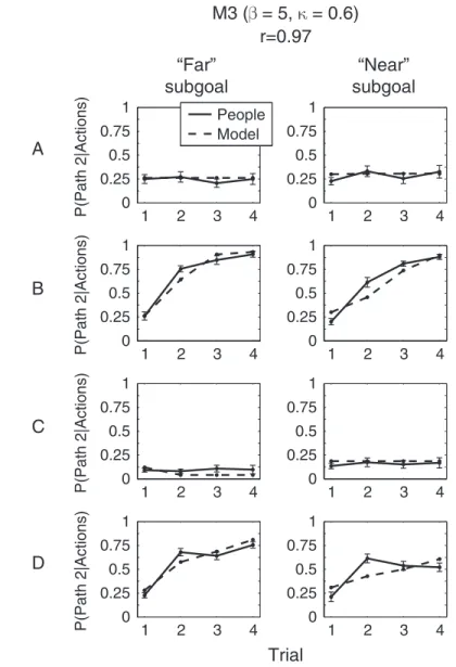
To test whether people’s judgments were consistent with these principles, Experiment 3 used a new task involving prediction of an agent’s future behavior, given examples of its behavior in the past. This experiment used simple maze-world versions of the scenarios described above. Our stimuli presented one or more trajectories in which the agent seemed to change direction at a single midpoint location along the way to a final goal, suggesting the possibility of a complex goal with a subgoal. We assessed whether subjects inferred a subgoal by asking them to predict the agent’s hypothetical trajectory starting from a different initial location; if they inferred a subgoal, they would predict a different, more indirect path than if they inferred only a simple final goal. Different conditions varied the amount of evidence for complex goals. In some cases, intended to suggest a simple goal to observers, the change in direction could be naturally explained by environmental factors (avoiding an obstacle) or as a correction from a small random path deviation. In other cases, observers saw multiple trajectories starting from different initial positions, all with the same intermediate switch point, which should strongly suggest a subgoal at that location. We compared people’s judgments in these different conditions with those of our Bayesian inverse planning models, using the models’ ability to predict future action sequences consistent with the goals inferred from earlier observed action sequences (Equation 2).
Method
Participants.
Participants were 23 members of the MIT subject pool, 14 female, 9 male. Stimuli.
Experiment 3 used a maze-world stimulus paradigm similar to Experiments 1 and 2. Fig. 9 shows all stimuli from Experiment 3. Each stimulus displayed a complete action