HAL Id: hal-02609769
https://hal.inrae.fr/hal-02609769
Submitted on 18 Jan 2021
HAL is a multi-disciplinary open access
archive for the deposit and dissemination of
sci-entific research documents, whether they are
pub-lished or not. The documents may come from
teaching and research institutions in France or
abroad, or from public or private research centers.
L’archive ouverte pluridisciplinaire HAL, est
destinée au dépôt et à la diffusion de documents
scientifiques de niveau recherche, publiés ou non,
émanant des établissements d’enseignement et de
recherche français ou étrangers, des laboratoires
publics ou privés.
Back to the future: dynamic full carbon accounting
applied to prospective bioenergy scenarios
Ariane Albers, Pierre Collet, Anthony Benoist, Arnaud Hélias
To cite this version:
Ariane Albers, Pierre Collet, Anthony Benoist, Arnaud Hélias. Back to the future: dynamic full carbon
accounting applied to prospective bioenergy scenarios. International Journal of Life Cycle Assessment,
Springer Verlag, 2020, 25 (7), pp.1242-1258. �10.1007/s11367-019-01695-7�. �hal-02609769�
Back to the future: Dynamic full carbon accounting applied to
prospective bioenergy scenarios
Ariane Albers 1,2,3,*, Pierre Collet 1, Anthony Benoist 3,4, Arnaud Hélias 2,5,6
1 IFP Energies nouvelles, 1 et 4 Avenue de Bois-Préau, 92852 Rueil-Malmaison, France 2 LBE, Montpellier SupAgro, INRA, UNIV Montpellier, Narbonne, France
3 Elsa, Research group for Environmental Lifecycle and Sustainability Assessment, Montpellier, France 4 CIRAD - UPR BioWooEB, Avenue Agropolis, F-34398 Montpellier, France
5 Chair of Sustainable Engineering, Technische Universität Berlin, Berlin, Germany
6 ITAP, Irstea, Montpellier SupAgro, Univ Montpellier, ELSA Research Group, Montpellier, France * Corresponding author, E-mail: ariane.albers@ifpen.fr
Purpose. Ongoing debates focus on the role of forest-sourced bioenergy within climate mitigation efforts, due to the long rotation lengths of forest biomass. Valuing sequestration is debated due to its reversibility; however, dynamic modelling of biogenic carbon (Cbio) flows captures both negative and positive emissions. The objective of this work is to respond to the key issue of timing sequestration associated with two opposed modelling choices (historic vs. future) in the context of dynamic LCA.
Methods. The model outputs of a partial-equilibrium model are used to inform prospective evaluations of the use of forest wood residues in response to an energy transition policy. Dynamic forest carbon modelling represents the carbon cycle between the atmosphere and technosphere: Cbio fixation and release through combustion and/or decay. Time-dependent characterisation is used to assess the time-sensitive climate change effects. The two Cbio sequestration perspectives for bioenergy (biomass use) and reference (no use) scenarios are contrasted to assess i) their temporal profiles, ii) their climatic consequences concerning complete (fossil + biogenic C) vs C-neutral (fossil C) approaches, and iii) the implications of comparing the two approaches with dynamic LCA. Results and discussion. Full lifetime carbon accounting confirms that Cbio entering the bioenergy system equals the Cbio leaving it in a net balance, but not within annual balances, which alter the atmospheric greenhouse gas composition. The impacts of the historic approach differed considerably from those of the future. Moreover, the
methane proportions. The chicken-egg dilemma arises in attributional LCA: as the forcing depends on the timing of the Cbio sequestration and its allocation to a harvest activity. A decision tree supported by case study applications provides general rules for selecting the adequate time-related modelling approach based the criteria of provision of wood and regrowth from managed and unmanaged forests, determined by the origin of biotic resources and related spheres. Conclusions. Excluding dynamic Cbio introduces under- (future) or over- (historic) estimation of the results, misleading mitigation results. Further research is needed to close the gap between forest stand and landscape level, addressing issues beyond the chicken-egg dilemma, and developing complete dynamic LCA studies.
1 2 3 4 5 6 7 8 9 10 11 12 13 14 15 16 17 18 19 20 21 22 23 24 25 26 27 28 29 30 31 32 33 34 35 36 37 38 39 40 41 42 43 44 45 46 47 48 49 50 51 52 53 54 55 56 57 58 59 60
Keywords: bioenergy; biogenic carbon; carbon sequestration; climate change; dynamic LCA
C Carbon GHG Greenhouse Gas
Cbio Biogenic carbon LTECV French Energy Transition for Green Growth Act CDM Clean Development Mechanism LULUCF Land Use, Land Use Change and Forestry CER Certified Emission Reduction N2O Nitrous Oxide
CFs Characterisation Factors PEM Partial-equilibrium model CH4 Methane RF Radiative Forcing CO2 Carbon dioxide TH Time Horizon
CO2-eq Carbon Dioxide Equivalent TIMES The Integrated Markal-Efom System EOL End-of-life UNFCCC United Nations Framework Convention on
Climate Change FoWooR Forest Wood Residues
1 2 3 4 5 6 7 8 9 10 11 12 13 14 15 16 17 18 19 20 21 22 23 24 25 26 27 28 29 30 31 32 33 34 35 36 37 38 39 40 41 42 43 44 45 46 47 48 49 50 51 52 53 54 55 56 57 58 59
The growing demand for alternative renewable energy carriers, to support a transition towards low carbon economies, has been supported since the 90s under the Kyoto Protocol, by international mechanisms such as the Clean Development Mechanism (CDM) and Certified Emission Reduction (CER) (UNFCCC 2019), as well as by EU legislation setting ambitious targets to reduce greenhouse gas (GHG) emissions (EC 2009; Scarlat et al. 2015). Incentives encourage the displacement of fossil carbon by means of biogenic carbon (Cbio), thus crediting (e.g. carbon offsets) the avoided equivalent fossil sourced emission.
Carbon flows are differentiated by their source of origin, as fossil from non-renewable and biogenic from renewable biomass sources. Alternative bioenergy pathways based on dedicated and residual lignocellulosic biomass (e.g. forest wood, short rotation coppice, maize stover, wheat straw, perennial grasses) are increasingly recognised as competitive advanced substitutes to displace fossil carbon and reduce the use of first generation energy crops, a desirable evolution under land-use and food security concerns (Wise et al. 2009; Rathmann et al. 2010; Harvey and Pilgrim 2011).
Ongoing debates focus on the role of forest-based bioenergy within the climate mitigation efforts, due to its long rotation lengths and thus long sequestration periods (Haberl et al. 2012; Cowie et al. 2013a). Despite the end-of-life (EOL) of biomass as biofuel combustion or wood incineration represents an instant release, the timing of Cbio sequestration in biomass may stretch over several decades (Zetterberg and Chen 2015). Yet, valuing temporary carbon sequestration (carbonremoval from the atmosphere and fixation in the biomass through photosynthesis) and storage (carbon retention in the technosphere) for bioenergy systems has long been questioned (Levasseur et al. 2012a; Brandão et al. 2013).
The Life Cycle Assessment (LCA) framework allows for a holistic assessment of potential climate change impacts (and other environmental impacts) of bioenergy systems, but conventionally from a static perspective (Guinée et al. 2002). Originally, temporal information is not processed by the computational structure of LCA (Heijungs and Suh 2002) and is excluded from the ISO standard (ISO 2006a, b). The global warming potential (GWP) method represents a relative measure of the sum of all inventoried instant to long-term GHG emissions fixed over a time horizon (TH), regardless of when in time the emissions occur (Benoist 2009; Levasseur et al. 2010). This static quality concerns also the Cbio flows, often excluded from life cycle inventories (LCI)
(Pawelzik et al. 2013). The conventional LCA approach is restricted to linear simplification and thus an inherent carbon neutrality (i.e. one unit of Cbio release is balanced thorough the same unit of Cbio sequestered) is
associated with the use of any type of biomass. Two main approaches for biomass-sourced products are well discussed in LCA literature, namely carbon neutral and carbon storage (Pawelzik et al. 2013), respectively applied to short-lived (bioenergy) and long-lived (e.g. wood construction materials) products. For bioenergy systems, the widely used carbon neutral approach is based on the abovementioned steady state assumption. The carbon neutral (C-neutral) approach excludes Cbio emissions from bioenergy with EOL modelled as combustion/ incineration, but includes fossil emissions for biofuel production (Johnson 2009; Agostini et al. 2014; Wiloso et al. 2016). Nonetheless, for forestry resources it has long been criticised as an erroneous
1 2 3 4 5 6 7 8 9 10 11 12 13 14 15 16 17 18 19 20 21 22 23 24 25 26 27 28 29 30 31 32 33 34 35 36 37 38 39 40 41 42 43 44 45 46 47 48 49 50 51 52 53 54 55 56 57 58 59 60
accounting approach (Searchinger et al. 2009; Haberl et al. 2012),
(Zetterberg and Chen 2015) does not necessarily mean CO2 neutral. Given the generalised C-neutral assumption, conventional LCA approaches disregard the temporal effects from sequestration in forestry systems, thus failing at linking both bioenergy and forest carbon modelling (Searchinger et al. 2009; Newell and Vos 2012; Røyne et al. 2016). From a national viewpoint, forest Cbio flows are ignored downstream (bioenergy combustion), as the C losses are accounted for at the upstream (i.e. land use, land use change and forestry - LULUCF) by means of the stock change method for global carbon pools used in national GHG inventory reports (IPCC 2006a; UNFCCC 2014). That is to say, emissions reported at the LULUCF are not reported in the bioenergy sector, to avoid double counting (Zanchi et al. 2010). For instance, CO2 emissions from biofuels are excluded from the EU Emission Trading System (Zetterberg and Chen 2015).
The temporary carbon storage approach, on the other hand, is optional for long-lived bioproducts (e.g. wood construction material), providing a benefit to delayed emissions from Cbio embedded in biomaterials. The ILCD Handbook (EC-JRC 2010) and the PAS2050 (BSI 2008) standard allow the accounting of emission delays over 100 years (i.e. postponement of radiative forcing - RF). Long-term storage beyond one century is not accounted for, but reported separately. The tonne-year-based Moura-Costa (Moura Costa and Wilson 2000) and Lashof (Fearnside et al. 2000) approaches, initially introduced in the context of LULUCF, have been discussed for product level applications (Korhonen et al. 2002; Levasseur et al. 2012b).
An alternative dynamic approach has been proposed in the context of the dynamic LCA method (Levasseur et al. 2010), featuring time-sensitive climate change impacts via the timing of fossil and biogenic flows. The timing difference of Cbio flows between sequestration and release, from and to the atmosphere, defines the period over which the carbon is embedded in the technosphere. During that period, the RF is postponed (for biomass resources with long rotation lengths and long-lived products) or eventually avoided through permanent stocks (Christensen et al. 2009; Vogtländer et al. 2014). The dynamic method was contrasted with the tonne-year approaches (Levasseur et al. 2012b) as well as with the GWP metric and other methods from the ILCD Handbook and PAS2050, used in classical LCA, showing significant variations in the results (Levasseur et al. 2012c).
Available methods, including the dynamic one, have been thoroughly discussed for valuing temporary carbon sequestration and storage for LCA bioenergy (Brandão et al. 2013, 2019), yet it was concluded that none of the current methods is preferred over the other, as the results still depend on a time horizon (TH) for the
characterisation. Nonetheless, a few methodology reports, such as the CML Handbook (Guinée et al. 2002), the ReCiPe methodology (Hischier et al. 2010) and the FAO EX-ACT tool (Grewer et al. 2017) described and compared with other carbon modelling tools in Colomb et al. (2012)
for CO2 of biogenic origin in specific studies.
The dynamic LCA method appears to be adequate, tackling the issue of timing biogenic elementary flows, as applied in several other studies of forest bioproducts (Fouquet et al. 2015; Daystar et al. 2016; Peñaloza et al. 2016, 2018; Demertzi et al. 2018), and more specifically of forest-bioenergy (Zetterberg and Chen 2015; Albers
1 2 3 4 5 6 7 8 9 10 11 12 13 14 15 16 17 18 19 20 21 22 23 24 25 26 27 28 29 30 31 32 33 34 35 36 37 38 39 40 41 42 43 44 45 46 47 48 49 50 51 52 53 54 55 56 57 58 59
consider the temporal profiles of Cbio flows. Temporary carbon storage is diluted by subtracting the amount of sequestered carbon from the emissions occurring at the end of the storage period, thus yielding a net zero emission. In contrast, carbon storage is reversible (i.e. reemitted) at some point in time, making it highly debatable whether or not assigning a value to it is justifiable (Levasseur et al. 2012a; Brandão et al. 2013). Yet, the dynamic method captures all the lifecycle emissions, including delays through time, by taking into account both the upstream (sequestration) and downstream (e.g. combustion/incineration, decay) flows.
The application of a dynamic LCA requires temporal emission profiles, i.e. the development of dynamic
inventories by timing each elementary flow (Collet et al. 2011). Cbio sequestration related with forest tree growth has been modelled, for instance, by means of a net carbon balance and linear distribution (Levasseur et al. 2012b), Gaussian normal distribution (Cherubini et al. 2011a; Cardellini et al. 2018), non-linear growth models such as the CARBINE model (De Rosa et al. 2017), the Schnute model (Cherubini et al. 2011b), or the
Chapman-Richards model (Yan 2018; Albers et al. 2019a).
Whatever modelling approach applied, the dynamic Cbio sequestration flows face a key accounting challenge, the so-called -and-egg (Levasseur et al. 2012c). It refers to an allocation issue to a harvest activity: the dynamic LCI can be modelled by considering a full biomass growth/rotation length before or after the harvest of said biomass. The former accounts for historic Cbio sequestration flows (forest growth occurs before logging) and the latter for future Cbio sequestration flows (forest re-regrowth occurs after logging by replanting new seedlings).
Published studies have applied the historic (Vogtländer et al. 2014; Zetterberg and Chen 2015; Demertzi et al. 2018; Albers et al. 2019a), future (Cherubini et al. 2011b, a; Levasseur et al. 2012b; Repo et al. 2015; Pingoud et al. 2016; De Rosa et al. 2017) and occasionally both (Levasseur et al. 2012c; Fouquet et al. 2015; Peñaloza et al. 2018) approaches. These opposed time perspectives yield different results, which require careful justification of the modelling choice. Future-oriented sequestration has been recommended for consequential LCA, and historic accounting for attributional LCA modelling (De Rosa et al. 2017). No universal guideline exists to date, on how to set the temporal boundaries of forest resource modelling or how to justify the use of one modelling approach over the other.
The objective of this study is thus to contrast both time-related modelling choices (before/historic vs.
after/future) for Cbio sequestration of forestry resources related with prospective bioenergy scenarios, to better comprehend the time-sensitive climate change effects in the context of the dynamic LCA framework.
Consequently, a detailed discussion is intended to deliver transparency and broaden understanding by exploring different cases, to support robust decision-making on the modelling choice.
This study challenges the C neutral and static assumptions for forest biomass resources with long rotation lengths by timing both Cbio sequestration and release flows (dynamic Cbio balance). An illustrative case study was developed based on data from a partial-equilibrium model (PEM) for the entire energy-transport sector in
1 2 3 4 5 6 7 8 9 10 11 12 13 14 15 16 17 18 19 20 21 22 23 24 25 26 27 28 29 30 31 32 33 34 35 36 37 38 39 40 41 42 43 44 45 46 47 48 49 50 51 52 53 54 55 56 57 58 59 60
France. The model-coupling principle, described in detail in Albers et al. (2019a), combines prospective energy system analysis with Cbio models to assess the time-sensitive potential climatic consequences of any energy policy scenario by means of a fossil + biogenic (C-complete) accounting. It enables accounting and
characterising time-dependent Cbio flows from emerging renewable energy pathways (i.e. biomass commodities) in the specific context of the dynamic LCA framework proposed by Levasseur et al. (2010).
Unlike classical LCA approaches, the functional unit expresses the national (here France) prospective energy demand, in GJ, per policy constraint and per year, over a given simulation period (here from 2019 to 2050), required to satisfy the energy consumption of end-users (industry, transport and households) across scenarios: the energy-mix (electricity and heat) and transport-biofuels (i.e. GJ per km travelled by a specific transportation means). The dynamic Cbio balance refers to the PEM functional unit by modelling the biogenic elementary flows, in t Cbio yr-1, of the supply commodity output forest wood residue (hereafter referred to as FoWooR), a biomass-sourced energy carrier used as a renewable raw material.
The two Cbio sequestration time perspectives for FoWooR are assessed, by contrasting: i) the different temporal profiles, ii) their time-dependent climatic consequences computed by C-complete vs C-neutral approaches and iii) the implications of comparing the two approaches with dynamic LCA.
LCA studies have previously been combined with PEM models to identify emerging technologies and energy pathways as well as to carry out consequential modelling in LCA implying changes in demand (Eriksson et al. 2007; Earles et al. 2013; Marvuglia et al. 2013; Vázquez-rowe et al. 2014; Menten et al. 2015a; Levasseur et al. 2017; Albers et al. 2019a). PEM models are key instruments to support robust decision-making by assessing in detail substitution alternatives and potential future energy pathways and their consequences on the market dynamic on specific sub-sectors (from the supply-and demand-side) and the environment (Gargiulo and Brian 2013; Nicolas et al. 2014). A commonly used PEM model generator is TIMES (MARKet Allocation-EFOM System; https://iea-etsap.org/). The model framework explores bottom-up linear optimisation pathways with a detailed technology database linking petroleum and biomass commodities with diverse conventional and refinery and innovative biomass conversion processes (Loulou et al. 2016).
We used the PEM model TIMES-MIRET, analysing the energy-mix (electricity and heat network) and transport sectors of metropolitan France (Lorne and Tchung-Ming 2012), following Albers et al. (2019a), to obtain prospective scenarios on the FoWooR commodity supply and the net GHG emissions (here fossil-sourced CO2 and N2O) of the entire energy-transport system assessed (detailed in the Supplementary Material). The provision of energy services to end-users encompasses biomass and crude oil extraction, refinery and bioprocess,
combustion at tailpipe, as well as heat and electricity network; including import-exports to/from other sectors. Besides conventional and renewable energy technologies, the TIMES-MIRET database contains emerging biomass conversion processes for second and third generation biofuels. Advanced biofuels from FoWooR, for instance, involve biochemical (ethanol) or thermo-chemical (synthetic/Fisher-Tropsch diesel) processes, depending on scenario simulations. Process pathways for other lignocellulosic biomass or algae involve transesterification or hydro treated pyrolysis oil.
1 2 3 4 5 6 7 8 9 10 11 12 13 14 15 16 17 18 19 20 21 22 23 24 25 26 27 28 29 30 31 32 33 34 35 36 37 38 39 40 41 42 43 44 45 46 47 48 49 50 51 52 53 54 55 56 57 58 59
TIMES-MIRET is calibrated to a reference policy scenario based on the 2009/28/EC Directive and National Renewable Energy Action Plan, as the business-as-usual (BAU) policy scenario. The policy scenario assessed in this study is based on the multi-annual energy programming of the 2015 French Energy Transition for Green Growth Act (MTES 2017) referred here as LTECV scenario. The LTECV scenario contains all constraints from BAU, including the updated targets for the transport sector: by 2030 minimum 15% renewable energy share and 30% reduction of fossil fuels, from 2020 maximum 7% share of first generation biofuels, and intermediate targets from 2018-2023 for advanced biofuels.
The dynamic Cbio balance represents the cycling carbon between the atmosphere and technosphere: Cbio fixation into the biomass through photosynthesis and the Cbio release through combustion and/or decay. Cbio fixation and Cbio decay gradually extend over longer periods, while Cbio combustion represents instant release emissions.
The Cbio fixation dynamic is computed by means of the forest carbon modelling approach of all main tree species of the wood supply chain in France, following Albers et al. (2019a), to predict the annual Cbio fixation from the atmosphere [t Cbioyr-1] over a given rotation length (provided in the Supplementary Material). The Cbio model refers to non-linear mean forest tree growth (Fekedulegn et al. 1999; Pretzsch 2009; Pommerening and Muszta 2015) based on the Chapman Richards model (Richards 1959) and allometric relations (Henry et al. 2013), including operationalised yield tables from long-term experimental forest plots (INRA/ONF/ENGREF 1984), featuring management regimes (e.g. thinning periods, rotation lengths and number of trees per plot). The growth, is characterised by a diminishing rate of Cbio sequestration as the tree matures, represented by a (classical) asymptotic and sigmoid growth curve. The modelling is based on homogenous growth of un-even aged and mixed management practices per forest stand. A key choice affecting the Cbio sequestration model concerns the data and models used to compute fixation (e.g. level of local-specificity of data used to fit the growth models, etc.), as well as the computation of the timing of sequestration.
Cbio decay dynamic is computed by a simple negative exponential equation, described in Albers et al. (2019a). CH4 emissions are estimated at 1.5% and 10%, respectively, for coarse woody debris and roots (Ros et al. 2013). The half-life decay values for aboveground and belowground are assumed at 8 and 30 years respectively (Montes and Cañellas 2006).
This study covers all FoWooR commodity outputs described in the TIMES-MIRET LTECV scenario, deriving from logging and thinning operations of commercial forests in France and collected for bioenergy use (i.e. cogeneration and transport biofuels). Additionally, a reference scenario is defined, against which the bioenergy is compared to evaluate potential climate change mitigation. According with Cowie et al. (2013), the reference may include forest management (e.g. for a different mix of products and services, or for conservation), but should exclude bioenergy. The Cbio reference in this study is referred to as
implies 100% of FoWooR left behind in the forest floor and emitted as CO2 and CH4, from both aerobic and anaerobic degradation.
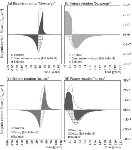
Fig. 1 shows a full lifetime accounting of Cbio flows (fixation and releases), under two scenarios concerning bioenergy and the no use (reference) scenarios of the commodity. In the bioenergy scenario, 30% of FoWooR
1 2 3 4 5 6 7 8 9 10 11 12 13 14 15 16 17 18 19 20 21 22 23 24 25 26 27 28 29 30 31 32 33 34 35 36 37 38 39 40 41 42 43 44 45 46 47 48 49 50 51 52 53 54 55 56 57 58 59 60
are accounted as non-collectable left behind biomass (Cacot et al. 2006; Lippke et al. 2011) and the collected portion (70% of logging residues) is further processed into advanced biofuels and electricity-heat cogeneration. The biofuel combustion is assumed to be emitted as CO2, while the Cbio decay releases from non-collectable/left-behind wood as CO2 and CH4 (to 30% in the bioenergy and to 100% in the no use scenarios). The Cbio flows from the belowground biomass corresponding to FoWooR are included by mass allocation of the residual part (37%) to the belowground root part (20%), resulting in 7.4% (Albers et al. 2019a).
Fig. 1. Full lifetime accounting of biogenic carbon (Cbio) from forest wood residues includes fixation, sequestration and
end-of-life releases through decay and/or combustion. The system boundary features two scenarios, the bioenergy (70% of
logging residues are combusted and 30% left behind to decay) and the (all residues are left in the forest
floor to decay)
Defining the temporal boundaries is as a key issue when describing the emission flows through time, particularly concerning Cbio from forestry resources (Levasseur et al. 2012b; Peñaloza et al. 2018). The LCA ISO
14040/14044 standard (ISO 2006a, b) refers to the setting of a time horizon (TH) for the impact characterisation (e.g. in the climate change category) in the goal and scope phase, but excludes any specification on the temporal emission profiles (i.e. temporally-differentiated LCI) of the modelled system.
Dynamic LCA implies defining a study TH, to establish the timing of the emission flows and impact
representations in the characterisation, by specifying: i) an inventory TH (hereafter referred to as LCI TH), and ii) an impact assessment TH (hereafter referred to as LCIA TH). The LCI TH describes when in time negative (Cbio sequestration) and positive (fossil and Cbio releases) flows occur over which the dynamic inventories are built. The LCIA TH is variable for time-dependent characterisation factors (CFs), when the evolution of the RF is evaluated and observed over time. By setting a specific end-year to the LCIA TH
(Levasseur et al. 2016) a temporal cut-off is performed, which is an unavoidable for comparison purposes and capturing the Cbio benefits (temporary sequestration) or impacts.
When coupling with any demand model, in this study with the PEM TIMES-MIRET, all Cbio emissions are aligned with the simulation years. The first carbon release represents t0, starting with the first combustion release (i.e. 2019) and ending with last year at t31 (i.e. 2050) of the PEM simulation.
1 2 3 4 5 6 7 8 9 10 11 12 13 14 15 16 17 18 19 20 21 22 23 24 25 26 27 28 29 30 31 32 33 34 35 36 37 38 39 40 41 42 43 44 45 46 47 48 49 50 51 52 53 54 55 56 57 58 59
All negative emissions from sequestration are adapted to the PEM simulation period going backwards or forward in time, depending on modelling approach applied. The historic approach allocate a full rotation length before the final harvest (preceding the wood harvest: first forest growth then tree felling) and the latter after (following the harvest: tree felling first then seeding new trees). The applied forest carbon model by Albers et al. (2019b) describes a maximum 200-year rotation length. Each PEM simulation year, within the range of t0-t31, represents a new harvest activity with its own sequestration curve. The total sequestration length for both historic and future perspectives sums up to 231 years, as shown in Fig. 2.
Fig. 2. Defining the time horizon of dynamic life cycle inventories concerning two opposed modelling time perspectives for biogenic sequestration
All positive biogenic and fossil releases from combustion (e.g. cogeneration or tail pipe) are instant, occurring within the same harvesting years over the range 0 to 31 years, while wood decay are long-term emissions distributed over several years, similar to Cbio sequestration. Under given half-life assumptions (see section 2.2) at least 60 years are required for the Cbio belowground biomass to decay. To avoid temporal cut-offs from long-term Cbio releases, it is recommended to extend the LCI TH, for instance, by adding 100 years to the last Cbio release (Fig. 2). Under such considerations, the net Cbio balance generates different LCI TH for historic and future time perspectives with 331 and 231 years respectively. Note that the 100-year TH is arbitrary, referring to the commonly reported TH in the IPCC Guidelines for National GHG Inventories (IPCC 2006b), following a political (e.g. UNFCCC Kyoto Protocol: CDM or CER projects) rather than a scientific decision (Fearnside 2002; Shine et al. 2005). For a full lifetime carbon accounting a generic approach is thus proposed by means of Eq. 1 for the historic and Eq. 2 for future sequestration.
Eq. 1
Eq. 2
The static method by means of the IPCC GWP metric (IPCC 2013) is not considered appropriate for dynamic carbon modelling, due to the fixed LCIA TH of 20 or 100 years. It assigns the same impact characterisation to all emissions, thus disregarding: i) the emission timing of each GHG emission in the atmosphere, ii) impacts beyond the fixed TH, providing a time preference to impacts (e.g. climate tipping points vs buying time for innovation), and iii) the inconsistency between LCI TH and LCIA TH; as confirmed by several authors (Kendall et al. 2009;
13; Cherubini et al. 2016). 1 2 3 4 5 6 7 8 9 10 11 12 13 14 15 16 17 18 19 20 21 22 23 24 25 26 27 28 29 30 31 32 33 34 35 36 37 38 39 40 41 42 43 44 45 46 47 48 49 50 51 52 53 54 55 56 57 58 59 60
On the other hand, the time-dependent CFs by Levasseur et al. (2010) are variable, with no fixed TH, representing the actual impacts for any given characterisation TH. The method assesses each emission flow following the year of its fixation or release. It overcomes the inconsistency between the different THs generated by the different emission years, thus enabling a consistent assessment between LCI TH and LCIA TH. Yet, the dynamic characterisation does imply setting an end-year to the impact assessment to account for the Cbio
sequestration benefits and allow transparent comparability among different scenarios. The end-year of the impact assessment would thus expressed the RF effects between the year of the emission release and the chosen fixed end-year (Levasseur et al. 2012c).
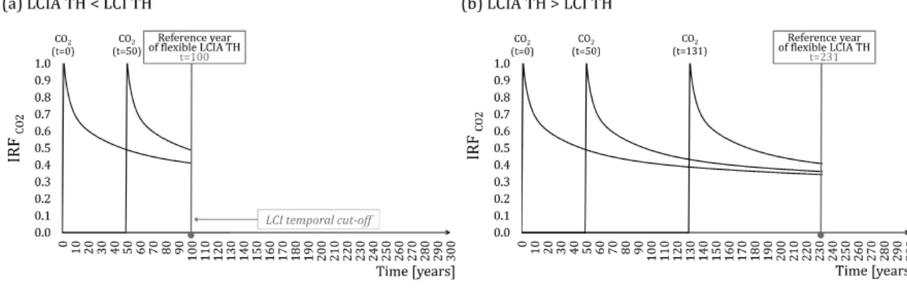
Consequently the study TH may cover (LCIA TH > LCI TH) or not (LCIA TH < LCI TH) all studied flows by the chosen end-year of the time-dependent characterisation, as exemplary shown in with the impulse-response function (Joos and Bruno 1996), predicting the decay of CO2 in the atmosphere. It will state, whether all flows are accounted for (full lifetime accounting), and which are eventually excluded (cut-off) from the study. A temporal cut-off appears when an LCIA TH is set for 100 years (Fig. 3a), while the LCI TH accounts for 131 years. It is to remark that matching THs (LCIA TH = LCI TH) may not project the forcing effect of the last emission at year 131, requiring the LCIA TH to be larger than LCI TH, as shown in Fig. 3b. For the present study, we defined a matching study TH (i.e. LCIA TH = LCI TH) per Cbio sequestration time perspective.
Fig. 3. Defining the study TH (temporal boundaries) by means of the life cycle inventory time horizon (LCI TH) and life cycle impact assessment time horizon (LCIA TH), illustrated with the impulse response function (IRF) of carbon dioxide
(CO2). The chosen LCIA TH may a) not cover or b) cover the elementary flows described within the LCI TH
Fig. 4 shows the Cbio balance of the FoWooR outputs from the LTECV policy scenario, contrasting both scenarios bioenergy and no use reference per historic and future modelling approach. The Cbio balance (darker shaded area in Fig. 4) consists of the sum of all negative and positive Cbio-CO2 and Cbio-CH4 flows (lighter shaded areas in Fig. 4) from Cbio fixation and release (combustion and/or decay). The Cbio flows are not yet converted into GHG emissions in this representation.
The temporal profiles for bioenergy and reference scenarios have different LCI THs (see Fig. 2): for the historic 331 years (Fig. 4 a,c) and for the future 231 years (Fig. 4 b,d), representing the PEM simulations period 1819-2150 and 2019-2250, respectively. The described LCI THs cover close to 100% of all emissions in the C
1 2 3 4 5 6 7 8 9 10 11 12 13 14 15 16 17 18 19 20 21 22 23 24 25 26 27 28 29 30 31 32 33 34 35 36 37 38 39 40 41 42 43 44 45 46 47 48 49 50 51 52 53 54 55 56 57 58 59
balance (remaining and 4E-5 t Cbio, depending on the scenario). The Cbio balance thus represents a full lifetime carbon accounting with no inventory cut-offs, as all embedded Cbio in the FoWooR is released back to the atmosphere. The chosen LCI TH confirm that the amount of Cbio entering the system is equal to the amount of Cbio leaving the system, which means that Cbio emissions can be considered neutral in the net balance, however not in the annual dynamic balance, ultimately affecting the atmospheric GHG composition.
Fig. 4. Life cycle carbon flows from dynamic biogenic carbon (Cbio), in t Cbio·yr-1, accounting for forest wood residues under
questration time perspectives
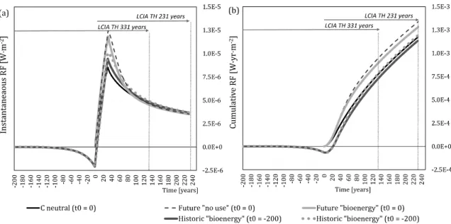
Fig. 5 shows the dynamic climate change impact assessment results of the LTECV policy per historic and future time perspectives, featuring C-neutral (fossil-sourced CO2 and N2O outputs from TIMES-MIRET), C-biogenic (Cbio balance) and C-complete (fossil + biogenic-sourced) curves for both bioenergy and no use FoWooR scenarios. Prior to the dynamic impact assessment all Cbio-CO2 and Cbio-CH4 flows were converted into the respective CO2 and CH4 GHG emissions, according to C-content in the molecules, 44/12 g CO2 g C-1 and 16/12 g CH4 g C-1 respectively. The instantaneous RF, in Fig. 5a,d describes the external net change in energy flows per watts square meter at the tropopause [W m-2], while the integral is given as cumulative RF [W yr m-2] in Fig. 5b,e and their relativisation to the cumulative CO2 as the relative RF [t CO2-eq] in Fig. 5c,f. Note that the impact representation of the two opposed modelling approaches have different t0 with different absolute calendar years of the PEM (i.e. 1819 for the historic and 2019 for the future approach).
1 2 3 4 5 6 7 8 9 10 11 12 13 14 15 16 17 18 19 20 21 22 23 24 25 26 27 28 29 30 31 32 33 34 35 36 37 38 39 40 41 42 43 44 45 46 47 48 49 50 51 52 53 54 55 56 57 58 59 60
The results of the C-biogenic flows per scenario and time perspective differ considerably. For the bioenergy scenario, the historic approach never fully reached positive, while the future approach never reached negative forcing effects. For the future approach, the instant and gradual releases from combustion and decay start simultaneously with the sequestration flows. The re-sequestration time of the emitted emissions is slow at the beginning and takes over two centuries (full rotation length) to compensate for the positive Cbio releases. For the historic approach, one full sequestration cycle is accounted before the first positive emission. Yet, the difference between the Cbio fixation and release curves decrease with increasing LCIA TH. Consequently, the further into the future the end-year of the impact assessment is set, the less significant do climatic benefits from Cbio sequestration become. Analogously, as demonstrated in the sensitivity analysis in Albers et al. (2019a), the shorter the rotation length of Cbio sequestration, the less significant are the negative forcing effects from Cbio. The accounting of the Cbio balance modifies the impacts of C-neutral assumptions, as shown in the C-complete curves in Fig. 5. The C-complete curves resemble the C-neutral ones, but with increasing or decreasing magnitude, given the two sequestration time perspectives. The same conclusions are drawn from the previous Cbio balance results (Fig. 4). The future sequestration lags behind the releases, while the opposite is the case for the historic perspective. The choice whether sequestration occurs before or after emissions thus considerably influences the results.
Moreover, a comparison between the bioenergy and the no use scenarios of both C-biogenic and C-complete, demonstrated that the impacts from 100% left behind FoWooR in the forest floor (reference), yielded higher forcing effects than for the bioenergy scenario in both historic and future modelling approaches. The emission flows are differentiated by their temporal distribution, which is either instantaneous (bioenergy) or gradual (decay). The anaerobic degradation processes produce CH4 emissions with higher radiative efficiency than CO2. Bioenergy and no use situations consider CH4, as shown in Fig. 1, but the reference has a higher proportion of CH4 emissions, as 100% of logging residues (including belowground biomass corresponding to FoWooR) are exposed to decay, compared to 30% for bioenergy. Consequently, the forcing effects of no use are higher than the bioenergy curve, as shown in Fig. 5.
1 2 3 4 5 6 7 8 9 10 11 12 13 14 15 16 17 18 19 20 21 22 23 24 25 26 27 28 29 30 31 32 33 34 35 36 37 38 39 40 41 42 43 44 45 46 47 48 49 50 51 52 53 54 55 56 57 58 59
Fig. 5. Instantaneous [W·m-2], cumulative [W·yr·m-2], and relative [t CO2-eq] radiative forcing (RF) effects from carbon (C)
emissions assessed for C-biogenic from forest wood residues, C-fossil (carbon neutral) and C-Complete (fossil + biogenic) under given bioenergy and no use (reference) scenarios and sequestration modelling time perspectives (historic and future rotation cycles)
The question arises on how to compare two opposing modelling approaches with different t0 and LCI THs (i.e. inventory time lengths). The application of the instantaneous or cumulative RF metrics allow a direct
comparison between the historic or future time perspectives and scenarios, regardless when t0 is set for the inventory and impact assessment. The results represent the actual impacts for any given GHG. On the other hand, the relative RF is based on the cumulative RF results relativized with the cumulative RF of the CO2 reference gas, fixed to an initial year (t0). The relative characterisation thus depends on the computation of a
1 2 3 4 5 6 7 8 9 10 11 12 13 14 15 16 17 18 19 20 21 22 23 24 25 26 27 28 29 30 31 32 33 34 35 36 37 38 39 40 41 42 43 44 45 46 47 48 49 50 51 52 53 54 55 56 57 58 59 60
fixed t0. Consequently, the two time perspectives with different t0 for Cbio sequestration are not comparable with the relative RF metric. It is most noticeable in the C-neutral curves in Fig. 5c, e, for instance by fixing the LCIA TH to 131 years, the impact would result in completely different magnitudes (i.e. 3.3E+9 for historic and 6.7E+9 for future perspectives). Following the complex comparison with dynamic CO2-eq results, the relative RF metric is excluded from the comparison undertaken in this section.
Fig. 6 shows a comparison of the instantaneous (Fig. 6a) and cumulative (Fig. 6b) RF effects of the historic and future C-complete results, including C-neutral, highlighting the choice of reference LCIA THs aligned with both historic LCI TH (331 years) and future LCI TH (231 years). Aligning the LCIA THs is performed to ensure a consistent comparison of results with different LCI THs in a specific year, and test the time-sensitivity due to the choice of the LCIA TH. In this comparison, t0 for historic is the year -200 and for future it the year 0. However, t0 for future could also refer to the year -200 (equal to the historic one), as the range between -200 and 0 for the future perspective does not account for any emissions, and is therefore not assessed with the dynamic
characterisation.
Concerning the cumulative results in Fig. 6b, an overall comparison denotes that the forcing effects for LCIA TH 231 are lower than for 331 years by around 60% for historic bioenergy (7.2E-4 and 1.1E-3 W yr m-2) and no use (7.7E-4 and1.2E-3 W yr m-2), by around 70% for future bioenergy (8.9E-4 and 1.3E-3 W yr m-2) and no use (9.4E-4 and 1.3E-3 W yr m-2), and by 65% for C-neutral (7.6E-4 and 1.2E-3 W yr m-2). The cumulative RF will continue increasing the longer the LCIA TH is set, due to the cumulated fraction of the CO2 gas remaining in the atmosphere, which has a very long residence time. For the dynamic results, the highest difference was thus found, as expected, among the historic and future modelling time perspectives. However, the margin between both FoWooR scenarios itself is considerable small ranging between 4% and 7%, depending on the LCIA TH and time perspective.
Fig. 6. Instantaneous [W·m-2] and cumulative [W·yr·m-2] radiative forcing (RF) effects from carbon (C) neutral (fossil
emissions only) and
C-(reference) scenarios and sequestration modelling time perspectives (historic and future rotation cycles). The arrows represent the setting of a life cycle impact assessment time horizon (LCIA TH) representing 231 and 331 years, for comparison purposes 1 2 3 4 5 6 7 8 9 10 11 12 13 14 15 16 17 18 19 20 21 22 23 24 25 26 27 28 29 30 31 32 33 34 35 36 37 38 39 40 41 42 43 44 45 46 47 48 49 50 51 52 53 54 55 56 57 58 59
The results in this study demonstrated that the modelling choice for timing forest growth and thus Cbio sequestration, before or after, matters. It was also demonstrated that Cbio accounting differs from C-neutral assumptions (Fig. 6), as Cbio sequestration can have a cooling (negative RF) effect with an historic perspective. However, when the sequestration lags behind release emissions in the future approach, a warming effect is observed, as pointed out by Helin et al. (2013) and confirmed in this study. After harvest activities, forest biomass needs to be replenished, which may take up to several centuries. Thus, modelling a full rotation length before the harvest yields a temporal carbon credit/benefit from an existing carbon stock, while modelling it after implies a temporal carbon debt/loss. In other words, carbon neutral results have been overestimated (historic) or underestimated (future) by the inclusion of dynamic Cbio flows.
The philosophical question from ancient Greece of whether the egg (sequestration) or the chicken (wood) comes first corresponds in the LCA methodology to an allocation issue: which sequestration, either before (historic) or after (future), should be attributed to a specific harvest? In this context, the chicken-egg dilemma arises in attributional LCA. In consequential LCA, the LCI modelling does not aim at allocating specific processes, such as Cbio sequestration, to specific products, such as harvested wood, but at representing the consequences of a change in decision or demand for the functional unit (Ekvall and Weidema 2004; Weidema et al. 2018). Therefore, the modelling principle for consequential LCA is to include all changes in Cbio flows related to a specific change and its effects on other systems, independently of their timing before or after the harvest. If the studied change relates to forest management (e.g. decrease of fertilisation rates), some modifications in Cbio flows can occur before harvest, but if this change relates to the harvest itself, consequences are likely to occur after harvesting (De Rosa et al. 2017).
In attributional LCA, the main consensual recommendation, e.g. from the ISO standard (ISO 2006a, b) or the ILCD handbook (EC-JRC 2010) to address an allocation issue, is to consider, when possible, an underlying causal physical relationship. In the case of managed forests, wood harvesting is possible because of the prior human activity of forest management; in that case, the time-related modelling should adopt an historic
perspective. Conversely, in the case of non-managed forests, biomass growth and harvest are not linked by a causal relationship, but if the forest is allowed to re-grow after harvest, this regrowth and the related Cbio sequestration occur because of the harvest; the time-related modelling should then adopt a future perspective. Fig. 7 provides a decision tree for the choice of time-related modelling based on these criteria, which generalises the proposed set of decision rules. Solving the chicken-egg dilemma is closely linked with another well-known issue in the LCA community, i.e. determining whether biotic resources are part of the ecosphere or the
technosphere, further explored in this section.
1 2 3 4 5 6 7 8 9 10 11 12 13 14 15 16 17 18 19 20 21 22 23 24 25 26 27 28 29 30 31 32 33 34 35 36 37 38 39 40 41 42 43 44 45 46 47 48 49 50 51 52 53 54 55 56 57 58 59 60
Fig. 7. Decision tree for the allocation of carbon sequestration to a harvest activity
The origin of a biotic resource is likely the most dominant question for Cbio modelling through time, together with identifying the appropriate Cbio sequestration approach. According with Lindeijer and colleagues, the origin of the biotic resource defines whether the modelled system stems from a man-made controlled culture (e.g. agriculture, aquaculture and silviculture) or from a natural ecosystem (Lindeijer et al. 2002). The authors applied an established definition for aquaculture (FAO 1997) to specify intensity of human activities in controlled systems, narrowing it down to two key interventions: increasing reproduction/yield rate (e.g. plant seedlings, supply hatcheries, irrigation, fertilisation) and mean life expectancy (e.g. mechanical or chemical weed control, phytosanitary control). The question on where the biotic resource extraction originates from, thus segregates the technosphere (anthropogenic) from the ecosphere (nature), and responds to which system the impacts from the extraction are allocated. The limits between the two spheres may therefore be determined to the level of human activities/interventions.
In the context of forest systems, managed and un-managed (including natural) forests should thus be
differentiated. Managed forests wood, fibre,
1 2 3 4 5 6 7 8 9 10 11 12 13 14 15 16 17 18 19 20 21 22 23 24 25 26 27 28 29 30 31 32 33 34 35 36 37 38 39 40 41 42 43 44 45 46 47 48 49 50 51 52 53 54 55 56 57 58 59
bioenergy and/or non-wood forest products (e.g. arabic gum, latex, resin, Christmas trees, cork, bamboo) (FAO 2010). The extraction of the biotic resource is possible due to planted seedlings (Lindeijer et al. 2002), meaning that the Cbio stocks are replenished and allowed to regrow. Additionally, in managed forests, species diversity is low. More than half of the French forests are monospecific and homogenous (IGN 2017). The human activity corresponds to reforestation, i.e. the reestablishment of a forest where it previously occurred, in contrast to afforestation where none previously existed (Lund et al. 2014). In sustainably managed forests, the carbon inventory does not decrease over time, as no more timber is removed than regrown (Lippke et al. 2011), as the
conserve a (FAO
2017).
In contrast to managed forests, natural forests evolved and reproduced [regenerated] itself naturally from organisms previously established [native species], and that has not been significantly altered by human activity
(FAO 2000, 2010). Natural forests are thus understood as previously/naturally existing, with insignificant or low level of human intervention. The same applies to un-managed forests, referring to abandoned/degraded forest or open woodland. A degraded forest features a reduction in quality, biomass, and species diversity induced by human activities (e.g. overexploitation, mismanagement) or natural disturbances (e.g. disease, pests, fires, windbreaks) (FAO 2000, 2011; Lund 2009, 2014).
From an economic/life cycle thinking viewpoint, managed forests (i.e. commercial forests) may be considered within the technosphere with the objective of providing and maximising the provision of biotic resources to meet future market demand. Un-managed forests (e.g. abandoned or degraded) may be considered as part of the ecosphere with no major economic intention. From an LCA viewpoint, un-managed forests could be considered equivalent to natural ones, as long as they are not part of a production system.
As per the previous segregation by the origin of the biotic resource between managed (technosphere) and un-managed/natural (ecosphere) forests, changes in land occupation are additional influencing criteria for modelling of Cbio sequestration (Fig. 7). Specific cases may be linked, for instance, to tree replacement with no forest cover (e.g. agriculture) and vice versa. Since prehistoric times, (agro)silvo-pastoral land use systems (i.e. wood-pasture habitats) have been performed in Europe, yet banned since the 1800s (Bergmeier et al. 2010). It confirms that forest landscapes have been exploited and modified far back in history, disturbed by clear-cuts, agricultural practices and active restorations (Vasseur 2012).
For these specific cases, a land-use baseline is necessary, particularly when assessing systems producing food, feed, fibre, timber and biofuels (Soimakallio et al. 2015). This baseline describes the dynamic development of ecosystem towards the achievable quasi-natural steady state (Milà i Canals et al. 2007; Koellner et al. 2013). Among the different approaches proposed to establish a land-use baseline, for the selection of which there is no established guidance (Koponen et al. 2018), it has been argued that the most adequate one consists in using the
(also referred to as natural relaxation) to estimate impacts from land use in attributional LCA (Soimakallio et al. 2015, 2016). A study of wood production across Canada (Head et al. 2018) suggested that the use of natural forest as a baseline may take 1000 years without anthropogenic disturbance to
1 2 3 4 5 6 7 8 9 10 11 12 13 14 15 16 17 18 19 20 21 22 23 24 25 26 27 28 29 30 31 32 33 34 35 36 37 38 39 40 41 42 43 44 45 46 47 48 49 50 51 52 53 54 55 56 57 58 59 60
approximate the steady-state carbon stock associated with a natural forest. Changes in land use and/or forest cover are beyond the scope of this work, as the chicken-egg dilemma does not apply to it.
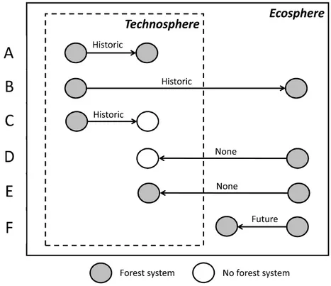
Different combinations of wood origin (ecosphere or technosphere), land cover (forest or non-forest) and type of forest (managed, unmanaged, natural, etc.) may be present on any particular Cbio sequestration modelling case study (Fig. 8).
Fig. 8. Possible cases (A to F) of carbon accounting scenarios associated with the provision of forest regrowth (forest system) and no provision of forest regrowth (no forest system). The direction of the arrows represents the relation between the previous and the current life cycles
Fig. 8 reflects the reference frame of a forest wood providing system under study, highlighting the relevance of identifying the previous state of land occupation. Based on the circumstances (state) of the previous life cycle, a rationale for applying the historic or future modelling approaches may be derived:
In cases A and B, harvested wood comes from a managed or unmanaged system, where the previous situation was a managed (i.e. in the technosphere) forest. In both cases, as there has been a human-induced Cbio sequestration, its modelling should be historical, as there is a history of sequestration. In case A, even if there are management changes among rotations, historical sequestration should be applied, as there is no land use change (forest to forest).
In case C, a special case of case A, in which a managed forest is harvested, and no provisions for regrowth are considered. As there is a history of sequestration, C accounting should be historical. In case D, a natural forest is harvested, and no provisions for regrowth are considered. Therefore, no
Cbio sequestration can be attributed to the harvested wood, but a total loss of the C stocked in the natural forest. 1 2 3 4 5 6 7 8 9 10 11 12 13 14 15 16 17 18 19 20 21 22 23 24 25 26 27 28 29 30 31 32 33 34 35 36 37 38 39 40 41 42 43 44 45 46 47 48 49 50 51 52 53 54 55 56 57 58 59
In case E, a natural forest is harvested and eventually converted into a managed technosphere system (forest to forest), and therefore no Cbio sequestration can be attributed to the harvested wood, but a total loss of the C stocked in the natural forest. After the management change is consolidated, for instance during a second cycle of technosphere forest, the situation would resemble case A.
In case F, a natural forest is harvested and allowed to regrow without interventions such as reforestation, and no intention to turn the system into a managed forest. A future accounting of the natural regrowth should be carried out. In case that the regrowth is subject to interventions, that would be case E.
The case of bioenergy in this study can be identified with case A in Fig. 8, as the biotic resource (here FoWooR) originates from a managed forest that has a history of consecutive sequestration cycles, and thus forms part of the technosphere. The modelling choice for sequestration we consider more coherent for this case, at least pertaining sustainable managed forests in France, is the historic perspective. Managed forests required long-term planning due to their nature of long rotation lengths, which should be credited with the historic sequestration accounting approach.
The forest cover in France has annually increased by 0.7% since 1985 (IGN 2017). It implies that managed forest is a net carbon sink rather than a net emitter. Future projections on standing wood volumes are based on historical datasets from long term field studies (yield tables with age and productivity classes) over the past centuries (INRA/ONF/ENGREF 1984) and statistical evaluations on potential future national availabilities from harvest behaviours and current production volumes, including losses and mortalities (Colin and Thivolle 2016). The additional annual carbon stocked per ha of land is expected to satisfy the anticipated increase in wood demand. A comparison with the TIMES-MIRET business as usual policy outputs (reference), following Albers et al. (2019a), showed that the FoWooR supply would increase gradually in the LTECV scenario, by 2.5% in the year 2030 and up to 17% in the year 2050. This increment reflects the actual potential availability of French forests to sustainably supply 12 additional Mm3 of wood (Valade et al. 2018).
The wood supply chain in France amounts for 57.3 Mm3yr-1 ( 16 Mha of which are managed forest, accounting for 31% of the land use), with 53% of the wood used for lumber, paper and pulpwood and 47% ( 27.3 Mm3) for various bioenergy pathways (Agreste 2016; Valade et al. 2018). The wood residues from logging or thinning operations, when collected for the bioenergy sector, are considered as co-products from the forest wood supply chain. The co-product are destined to meet the raw material requirements of second generation biofuels and the energy mix, with on-site co-generation and other sectors such as domestic heating with pellets and wood chips, or blended transport-fuels with bioethanol and biodiesel.
A continuous sustainable forest growth and harvest, will most likely not increase the removal of FoWooR due to displacement of fossil fuels (Lippke et al. 2011). It has been stated that increases in wood use for bioenergy
and actual production (Valade et al. 2018). However, it may lead to intensifying forest management practices
1 2 3 4 5 6 7 8 9 10 11 12 13 14 15 16 17 18 19 20 21 22 23 24 25 26 27 28 29 30 31 32 33 34 35 36 37 38 39 40 41 42 43 44 45 46 47 48 49 50 51 52 53 54 55 56 57 58 59 60
and any additional mobilisation may imply the use of quality wood with high added value (dedicated biomass) for bioenergy.
Accounting for dynamic biogenic flows from forest biomass allows valuing Cbio sequestration of forest-bioenergy systems. Cbio sequestration postpones RF over several decades (cooling effect). The negative forcing effects, however, depend on the timing of sequestration. When the sequestration lags behind the releases (future sequestration cycle), the positive emissions overtake the negative with subsequent opposite effects, namely warming (positive RF). A carbon debt is created and it takes a full rotation length to compensate for the caused GHG costs. As demonstrated in this study, excluding the dynamic features of Cbio flows introduces bias and may mislead decision support. Forest ecosystems are dynamic and mitigation targets require dynamic approaches, showcasing time-dependency of carbon flows, as well as the time-sensitive implications for climate change. Carbon neutrality is not an option for modelling biotic resources with long rotation lengths. The dynamic LCA method is a constructive approach for timing fossil and Cbio flows both upstream and downstream the supply chain/life cycle of bio-based products. Dynamic models are closer to real applications compared with linear assumptions or default carbon stock values.
This study was concerned with finding a solution to the allocation issue associated with the chicken-egg dilemma of Cbio sequestration, attributing a future or historic perspective to a specific forestry biomass harvest. This study did not address modelling challenges associated with land use change, as those are beyond the chicken-egg dilemma. A decision tree (Fig. 7) supports the choice of time-related modelling based on a generalised set of decision rules for attributional approaches underlined by different cases (Fig. 8). Our proposals are limited to the comparison of prospective bioenergy scenarios at the product level. The dynamic at the landscape level may differ from those at the product level, and therefore further research is needed to close the gap between forest stand and landscape levels. Moreover, consequences on the soil organic carbon dynamic over time due to an increased demand of forest wood residues have not been considered. In a broader sense, such exploitation might affect forest ecosystem services involving biodiversity and the sustainable provision of goods and services (e.g. soil productivity and ecosystem functioning) in the long term. Further research is needed to respond to this concern, by addressing changes of carbon stock in the soil (in this study, for instance, we included decay of wood biomass in soil), but also by performing a complete LCA study including other impact categories.
Agostini A, Giuntoli J, Boulamanti A (2014) Carbon accounting of forest bioenergy critical literature review. EC JRC Scietific policy reports Rep EUR 25354 1 87. doi: 10.2788/29442
Agreste (2016) Forêts,
http://agreste.agriculture.gouv.fr/enquetes/forets-bois-et-derives/. Accessed 12 Dec 2017
Albers A, Collet P, Lorne D, et al (2019a) Coupling partial-equilibrium and dynamic biogenic carbon models to assess future transport scenarios in France. Appl Energy 239:316 330. doi:
10.1016/j.apenergy.2019.01.186
Albers A, Collet P, Benoist A, Hélias A (2019b) Data and non-linear models for the estimation of biomass
1 2 3 4 5 6 7 8 9 10 11 12 13 14 15 16 17 18 19 20 21 22 23 24 25 26 27 28 29 30 31 32 33 34 35 36 37 38 39 40 41 42 43 44 45 46 47 48 49 50 51 52 53 54 55 56 57 58 59
cas de la première génération. PhD thesis. École Nationale Supérieure des Mines de Paris
Bergmeier E, Petermann J, Schröder E (2010) Geobotanical survey of wood-pasture habitats in Europe: Diversity, threats and conservation. Biodivers Conserv 19:2995 3014. doi: 10.1007/s10531-010-9872-3 Brandão M, Kirschbaum MUF, Cowie AL, Hjuler SV (2019) Quantifying the climate change effects of
bioenergy systems: Comparison of 15 impact assessment methods. GCB Bioenergy 1 17. doi: 10.1111/gcbb.12593
Brandão M, Levasseur A, Kirschbaum MUF, et al (2013) Key issues and options in accounting for carbon sequestration and temporary storage in life cycle assessment and carbon footprinting. Int J Life Cycle Assess 18:230 240. doi: 10.1007/s11367-012-0451-6
BSI (2008) Guide to PAS 2050: How to assess the carbon footprint of goods and services. British Standard. London
Cacot E, Eisner N, Charnet F, et al (2006) La récolte raisonnée des rémanents en forêt. ADEME-Agence de Cardellini G, Mutel CL, Vial E, Muys B (2018) Temporalis, a generic method and tool for dynamic life cycle
assessment. Sci Total Environ 645:585 595. doi: 10.1016/j.scitotenv.2018.07.044
Cherubini F, Fuglestvedt J, Gasser T, et al (2016) Bridging the gap between impact assessment methods and climate science. Environ Sci Policy 64:129 140. doi: 10.1016/j.envsci.2016.06.019
Cherubini F, Peters GP, Berntsen T, et al (2011a) CO2 emissions from biomass combustion for bioenergy: atmospheric decay and contribution to global warming. GCB Bioenergy 3:413 426. doi: 10.1111/j.1757-1707.2011.01102.x
Cherubini F, Strømman AH, Hertwich E (2011b) Effects of boreal forest management practices on the climate impact of CO2 emissions from bioenergy. Ecol Modell 223:59 66. doi: 10.1016/j.ecolmodel.2011.06.021 Christensen TH, Gentil E, Boldrin A, et al (2009) C balance , carbon dioxide emissions and global warming
potentials in LCA-modelling of waste management systems. ISWA 707 715. doi: 10.1177/0734242X08096304
ADEME/IGN/FCBA. Paris
Collet P, Hélias A, Lardon L, Steyer J-P (2011) Time and Life Cycle Assessment: How to Take Time into Account in the Inventory Step? 618. doi: 10.1007/s11367-013-0678-x
Colomb V, Bernoux M, Bockel L, et al (2012) Review of GHG calculators in agriculture and forestry sectors: A guideline for appropriate choice and use of landscape based tools.
ADEME-Cowie A, Berndes G, Smith T (2013a) On the timing of greenhouse gas mitigation benefits of forest-based bioenergy. ExCo:2013:04. IEA Bioenergy. Dublin
Cowie A, Berndes G, Smith T (2013b) On the Timing of Greenhouse Gas Mitigation Benefits of Forest-Based Bioenergy. Dublin
Daystar J, Venditti R, Kelley SS (2016) Dynamic greenhouse gas accounting for cellulosic biofuels: implications of time based methodology decisions. Int J Life Cycle Assess 1 15. doi: 10.1007/s11367-016-1184-8 De Rosa M, Schmidt J, Brandão M, Pizzol M (2017) A flexible parametric model for a balanced account of
forest carbon fluxes in LCA. Int J Life Cycle Assess 22:172 184. doi: 10.1007/s11367-016-1148-z Demertzi M, Paulo JA, Faias SP, et al (2018) Evaluating the carbon footprint of the cork sector with a dynamic
approach including biogenic carbon flows. Int J Life Cycle Assess 23:1448 1459. doi: 10.1007/s11367-017-1406-8
Earles JM, Halog A, Ince P, Skog K (2013) Integrated economic equilibrium and life cycle assessment modeling for policy-based consequential LCA. J Ind Ecol 17:375 384. doi: 10.1111/j.1530-9290.2012.00540.x
EC-Environmental Impact Assessment methodologies for use in Life Cycle Assessment. European Commission Joint Research Centre (JRC) contract, Ispra
EC (2009) DIRECTIVE 2009/28/EC on the promotion of the use of energy from renewable sources and amending and subsequently repealing Directives 2001/77/EC and 2003/30/EC
Ekvall T, Weidema BP. (2004) System Boundaries and Input Data in Consequential Life Cycle Inventory Analysis. Int J Life Cycle Assess 9:161 171. doi: 10.1065/Ica2004.03.148
Eriksson O, Finnveden G, Ekvall T, Björklund A (2007) Life cycle assessment of fuels for district heating: A
1 2 3 4 5 6 7 8 9 10 11 12 13 14 15 16 17 18 19 20 21 22 23 24 25 26 27 28 29 30 31 32 33 34 35 36 37 38 39 40 41 42 43 44 45 46 47 48 49 50 51 52 53 54 55 56 57 58 59 60
comparison of waste incineration, biomass- and natural gas combustion. Energy Policy 35:1346 1362. doi: 10.1016/j.enpol.2006.04.005
FAO (1997) Review of the state of the world fishery resources: Marine Fisheries. FAO-Food and Agricultural Organization of the United Nations, Rome
FAO (2010) Terms and Definitions. Global Forest Resource Assessment. Working Paper 144/E. Forest Resources Assessment Programme, Food and Agriculture Organization of the United Nations, Rome FAO (2017) Natural Forest Management: Sustainable forest management. In: Food Agric. Organ. United
Nations. http://www.fao.org/forestry/sfm/en/. Accessed 30 Jan 2019
FAO (2000) Asia-Pacific Forestry Commission: Development of National-Level Criteria and Indicators for the Sustainable Management of Dry Forests of Asia: Workshop Report. FAO-Food and Agricultural Organization of the United Nations, Bangkok
FAO (2011) Assessing forest degradation: Towards the development of globally applicable guidlines. Food and Agriculture Organization, Rome
Fearnside PM (2002) Why a 100-Year Time Horizon should be used for GlobalWarming Mitigation Calculations. Mitig Adapt Strateg Glob Chang 7:19 30. doi: 10.1023/A:1015885027530
Fearnside PM, Lashof DA, Moura-Costa P (2000) Accountingfor time in mitigating global warming through land-use change and forestry. Kluwer Acad Publ 5:239 270. doi: 10.1023/A:1009625122628
Fekedulegn D, Mac Siurtain MP, Colbert JJ (1999) Parameter estimation of nonlinear growth models in forestry. Silva Fenn 33:327 336. doi: 10.14214/sf.653
Fouquet M, Levasseur A, Margni M, et al (2015) Methodological challenges and developments in LCA of low energy buildings: Application to biogenic carbon and global warming assessment. Build Environ 90:51 59. doi: 10.1016/j.buildenv.2015.03.022
Gargiulo M, Brian O (2013) Long-term energy models: Principles, characteristics, focus, and limitations. WIREs Energy Env 2:158 177. doi: 10.1002/wene.62
Grewer U, Bockel L, Schiettecatte L-S, Bernoux M (2017) Ex-Ante Carbon-balance Tool (EX-ACT). Quick Guidance. Rome: Food and Agriculture Organization of the United Nations
Guinée JB, Gorrée M, Heijungs R, et al (2002) Handbook on life cycle assessment. Operational guide to the ISO standards. I: LCA in perspective. IIa: Guide. IIb: Operational annex. III: Scientific background. Kluwer Academic Publishers, Dordrecht
Haberl H, Sprinz D, Bonazountas M, et al (2012) Correcting a fundamental error in greenhouse gas accounting related to bioenergy. Energy Policy 45:18 23. doi: 10.1016/j.enpol.2012.02.051
Harvey M, Pilgrim S (2011) The new competition for land: Food, energy, and climate change. Food Policy 36:S40 S51. doi: 10.1016/j.foodpol.2010.11.009
Head M, Bernier P, Levasseur A, et al (2018) Forestry carbon budget models to improve biogenic carbon accounting in life cycle assessment. J Clean Prod 213:289 299. doi: 10.1016/J.JCLEPRO.2018.12.122 Heijungs R, Suh S (2002) The computational structure of life cycle assessment. Kluwer Acad Publ 7:314 314.
doi: 10.1007/BF02978899
Helin T, Sokka L, Soimakallio S, et al (2013) Approaches for inclusion of forest carbon cycle in life cycle assessment - A review. GCB Bioenergy 5:475 486. doi: 10.1111/gcbb.12016
Henry M, Bombelli A, Trotta C, et al (2013) GlobAllomeTree: International platform for tree allometric equations to support volume, biomass and carbon assessment. IForest 6:326 330. doi: 10.3832/ifor0901-006
Hischier R, Weidema B, Althaus H-J, et al (2010) Implementation of Life Cycle Impact Assessment Methods Data v2.2 (2010)
IGN (2017) Le mémento inventaire forestier édition 2017. In:
IGN-https://inventaire-forestier.ign.fr/IMG/pdf/memento_2017.pdf. Accessed 20 Jul 2018
INRA/ONF/ENGREF (1984) Tables de production pour les forêts françaises, 2e édition. INRA-Centre National de Recherche Forestières, ONF- Office National des Forêts, EGREF- Ecole Nationale du Génie rural, des Eaix et des Forêts, Nancy
IPCC (2006a) Chapter 4. Agriculture, forestry and other land use. In: Eggleston S, Buendia L, Miwa K, et al. (eds) 2006 IPCC Guidelines for National Greenhouse Gas Inventories. Intergovernmental Panel on Climate Change, Prepared by the National Greenhouse Gas Inventories Programme
IPCC (2006b) IPCC guidelines for national greenhouse gas inventories. Chapter 4. agriculture, forestry and other land use 1 2 3 4 5 6 7 8 9 10 11 12 13 14 15 16 17 18 19 20 21 22 23 24 25 26 27 28 29 30 31 32 33 34 35 36 37 38 39 40 41 42 43 44 45 46 47 48 49 50 51 52 53 54 55 56 57 58 59
IPCC (2013) Climate Change 2013 The Physical Science Basis. Contribution of Working Group I to the Fifth Assessment Report of the Intergovernmental Panel on Climate Change. Cambridge University Press, Cambridge and New York
ISO (2006a) ISO 14040 Environmental management Life cycle assessment Principles and framework. The International Standards Organisation. Geneva
ISO (2006b) ISO 14044 Environmental management Life cycle assessment Requirements and guidelines. The International Standards Organisation. Geneva
Johnson E (2009) Goodbye to carbon neutral: Getting biomass footprints right. Environ Impact Assess Rev 29:165 168. doi: 10.1016/j.eiar.2008.11.002
Joos F, Bruno M (1996) Pulse response functions are cost-efficient tools to model the link between carbon emissions, atmospheric CO2 and global warming. Phys Chem Earth 21:471 476. doi: 10.1016/S0079-1946(97)81144-5
Jørgensen S V, Hauschild MZ (2013) Need for relevant timescales when crediting temporary carbon storage. Int J Life Cycle Assess 747 754. doi: 10.1007/s11367-012-0527-3
Kendall A, Davis A, Studies T, et al (2009) Accounting for time-dependent effects in biofuel life cycle greenhouse gas emissions calculations. Environ Sci Technol 43:7142 7147. doi: 10.1021/es900529u Koellner T, de Baan L, Beck T, et al (2013) Principles for life cycle inventories of land use on a global scale. Int
J Life Cycle Assess 18:1203 1215. doi: 10.1007/s11367-012-0392-0
Koponen K, Soimakallio S, Kline KL, et al (2018) Quantifying the climate effects of bioenergy Choice of reference system. Renew Sustain Energy Rev 81:2271 2280. doi: 10.1016/j.rser.2017.05.292
Korhonen R, Pingoud K, Savolainen I, Matthews R (2002) The role of carbon sequestration and the tonne-year approach in fulfilling the objective of climate convention. Environ Sci Policy 5:429 441. doi:
10.1016/S1462-9011(02)00091-6
Levasseur A, Bahn O, Beloin-Saint-Pierre D, et al (2017) Assessing butanol from integrated forest biorefinery: A combined techno-economic and life cycle approach. Appl Energy 1 13. doi:
10.1016/j.apenergy.2017.04.040
Levasseur A, Brandão M, Lesage P, et al (2012a) Valuing temporary carbon storage. Nat Clim Chang 2:1 3. doi: 10.1038/nclimate1335
Levasseur A, Cavalett O, Fuglestvedt JS, et al (2016) Enhancing life cycle impact assessment from climate science: Review of recent findings and recommendations for application to LCA. Ecol Indic 71:163 174. doi: 10.1016/j.ecolind.2016.06.049
Levasseur A, Lesage P, Margni M, et al (2010) Considering time in LCA: Dynamic LCA and its application to global warming impact assessments. Environ Sci Technol 44:3169 3174. doi: 10.1021/es9030003 Levasseur A, Lesage P, Margni M, et al (2012b) Assessing temporary carbon sequestration and storage projects
through land use, land-use change and forestry: comparison of dynamic life cycle assessment with ton-year approaches. Clim Change. doi: 10.1007/s10584-012-0473-x
Levasseur A, Lesage P, Margni M, Samson R (2012c) Biogenic Carbon and Temporary Storage Addressed with Dynamic Life Cycle Assessment. J Ind Ecol 17:117 128. doi: 10.1111/j.1530-9290.2012.00503.x Lindeijer E, Müller-Wenk R, Bengt S (2002) Impact Assessment of Resources and Land Use. In: de Haes HAU,
Finnveden G, Goedkoop M, et al. (eds) Life-Cycle Impact Assessment: Striving towards Best Practice. Society of Environmental Toxicology and Chemistry (SETAC), pp 11 64
Lippke B, Oneil E, Harrison R, et al (2011) Life cycle impacts of forest management and wood utilization on carbon mitigation: knows and unknowns. Carbon Manag 2:303 333
Lorne D, Tchung-Ming S (2012) The French biofuels mandates under cost uncertainty an assessment based on robust optimization. IFPEN. Rueil-Malmaison
Loulou R, Lehtilä A, Kanudia A, et al (2016) Documentation for the TIMES Model PART II: Reference Manual. ETSAP-Energy Technology Systems Analysis Programme
Lund HG (2014) What is a forest? Definitions do make a difference an example from Turkey. Eurasscience Journals 2:1 8
Lund HG (2009) What is a degraded forest? 1. White paper prepared for FAO. Forest Information Services, Gainesville
Lund MT, Berntsen TK, Fuglestvedt JS (2014) Climate impacts of short-lived climate forcers versus
CO<inf>2</inf> from biodiesel: A case of the EU on-road sector. Environ Sci Technol 48:14445 14454. doi: 10.1021/es505308g 1 2 3 4 5 6 7 8 9 10 11 12 13 14 15 16 17 18 19 20 21 22 23 24 25 26 27 28 29 30 31 32 33 34 35 36 37 38 39 40 41 42 43 44 45 46 47 48 49 50 51 52 53 54 55 56 57 58 59 60


![Fig. 5. Instantaneous [W·m -2 ], cumulative [W·yr·m -2 ], and relative [t CO 2 -eq] radiative forcing (RF) effects from carbon (C) emissions assessed for C-biogenic from forest wood residues, C-fossil (carbon neutral) and C-Complete (fossil + biogenic) u](https://thumb-eu.123doks.com/thumbv2/123doknet/13803999.441290/14.892.228.696.106.862/instantaneous-cumulative-relative-radiative-emissions-assessed-biogenic-complete.webp)