HAL Id: hal-01655085
https://hal.inria.fr/hal-01655085
Submitted on 4 Dec 2017
HAL is a multi-disciplinary open access
archive for the deposit and dissemination of
sci-entific research documents, whether they are
pub-lished or not. The documents may come from
teaching and research institutions in France or
abroad, or from public or private research centers.
L’archive ouverte pluridisciplinaire HAL, est
destinée au dépôt et à la diffusion de documents
scientifiques de niveau recherche, publiés ou non,
émanant des établissements d’enseignement et de
recherche français ou étrangers, des laboratoires
publics ou privés.
Some highlights on Source-to-Source Adjoint AD
Laurent Hascoët
To cite this version:
Laurent Hascoët. Some highlights on Source-to-Source Adjoint AD. NIPS 2017 - workshop The future
of gradient-based machine learning software & techniques, Dec 2017, Long Beach, Californie, United
States. pp.1-5. �hal-01655085�
Some highlights on Source-to-Source Adjoint AD
Laurent Hascoët
Université Côte d’Azur, INRIA, France [email protected]
Abstract
Algorithmic Differentiation (AD) provides the analytic derivatives of functions given as programs. Adjoint AD, which computes gradients, is similar to Back Propagation for Machine Learning. AD researchers study strategies to overcome the difficulties of adjoint AD, to get closer to its theoretical efficiency. To promote fruitful exchanges between Back Propagation and adjoint AD, we present three of these strategies and give our view of their interest and current status.
1
Adjoint AD models
Algorithmic Differentiation (AD) [9, 14] is one way to obtain the analytical derivatives of a vector function F : X ∈ IRn 7→ Y ∈ IRm, when this function is provided as an algorithm. There are
other ways, such as differentiating the mathematical equations that the algorithm implements, if they exist. For AD the algorithm is the function: its run-time sequence of instructions is a composition of elementary functions that define the function. By applying the chain rule of calculus, AD builds a new sequence of instructions and eventually a new algorithm that computes the desired derivatives. Using AD, one can obtain first-order derivatives as well as higher-order or Taylor developments. Being based on the chain rule, these derivatives are analytic, meaning exact up to machine precision and free of the approximation errors that would result from other approaches, such as divided differences ˙Y ' (F (X + h ∗ ˙X) − F (X))/h. Yet their algorithmic cost remains similar to divided differences, and even much cheaper in the case of gradients.
Focusing on first-order derivatives from now on, associativity of matrix multiplication implies that the chain rule can be applied in various orders. Among those are two extremes:
• Derivative matrices can be multiplied forward, as the original program goes. This is called the tangent mode of AD. One provides one (or several) initial direction vector ˙X in the input space of the program, and the tangent differentiated code progressively computes the derivatives of every intermediate variable with respect to the inputs, along direction ˙X. Upon completion, the tangent code has computed into ˙Y the directional first-order derivative of the result Y with respect to X, at the given point X and along the given direction ˙X. Notice that the divided differences approach is by essence tightly bound to tangent AD, as it also goes from one given ˙X to ˙Y . Complexity-wise and like divided differences, the run-time of the tangent code is only a small multiple (1 to 3) of the original code. Computing all first-order derivatives of this vector function F : IRn → IRmrequires n runs of the
tangent code along the n vectors of the Cartesian basis of the input space.
• Derivative matrices can also be multiplied backwards. This is called the adjoint (or reverse) mode of AD. Given one (or several) weighting Y in the output space, the adjoint differ-entiated code progressively computes the derivatives of the scalar (Y |Y ) with respect to every intermediate variable, in the reverse of the original program execution order. Upon completion, the adjoint code has computed into X the gradient with respect to X of the func-tion (Y |F (X)). Divided differences are unable to emulate adjoint mode. Complexity-wise,
the run-time of the adjoint code is also a small multiple (slightly higher than for tangent code, 5 to 10 in practice) of the original code. Computing all first-order derivatives of F : IRn→ IRmrequires m runs of the adjoint code along the m vectors of the Cartesian
basis of the output space. Still, computing derivatives in reverse order poses additional technical problems that we will discuss later.
It turns out that many applications actually require a gradient (m = 1) or more generally m n. In that case adjoint mode is remarkably more efficient than tangent mode or than divided differences approximation. Primarily in view of applications such as gradient-based optimization or parameter estimation, AD researchers have spent considerable effort in building efficent adjoint codes. In Machine Learning, gradients are crucial for training neural networks, and “Back Propagation”, a close cousin of adjoint AD, has been recognized as a key technology. To investigate fruitful exchanges between Back Propagation and adjoint AD, we’d like to give here a few highlights on adjoint AD technology, and more precisely about AD tools that provide the adjoint mode through Source-to-Source Transformation (ST-AD).
There are many possible architectures to implement the backward computation of adjoint AD [5]. We call them adjoint AD models. An AD tool will implement (at least) one of these models. We like to
Figure 1: Adjoint AD forward and backward sweeps illustrate the model implemented by our
tool Tapenade [11] and also by Ope-nAD [16] by figure 1: since the deriva-tive propagation goes backwards, the ad-joint code must first run the original code to memorize the control flow that will be
used backwards. We show this “forward sweep” as a thick arrow to the right. Only then can derivative computation start, retrieving control flow information on the way. We show this “backward sweep” as a thick arrow to the left. Think of an original instruction and its derivative counterpart as aligned vertically. The derivative of an instruction may in general need the values that are used by the original instruction. If these needed values are overwritten by the sequel of the forward sweep, we must devise a mechanism, symbolized by the few red arrows, to make them available again during the backward sweep. In our model, this is basically done by storage. Other models exist that use recomputation [7], that we will not discuss here for the sake of brevity. In figure 1, arrow thickness also symbolizes storage and retrieval of these intermediate values. This is the bottleneck of adjoint AD, as this storage grows linearly with the program run time. In the next sections we will discuss techniques that cope with this issue: static Data-Flow analysis can reduce significantly the amount of storage needed, but still growing linearly with run time. Checkpointing is a memory/recomputation tradeoff that can make the storage grow only logarithmically with run time. In special cases such as Fixed-Point loops, specialized techniques can also reduce this storage drastically.
Before that, we close this section with a contrast with AD models based on Operator-Overloading (OO-AD). In OO-AD tools such as AdolC [17], dco [13], CoDiPack [1]. . . , the forward sweep additionally records every executed instruction into a “tape”, in a format resembling three-address code. The backward sweep doesn’t exist as a source any more. Rather, the tape is interpreted backwards by a special program that computes the derivatives. The advantage is that the tape format is easier to generate than it is to build the source of a reverse sweep, so that OO-AD can address more sophisticated application languages such as C++. It takes extra run-time to write this tape and the tape itself cannot be exposed to the compiler for optimization, however OO-AD tools are making impressive progress to cope with that. The main drawback is that the tape is much larger than the data recorded by ST-AD. Consequently the techniques in the next sections can be of value also for OO-AD.
In the small world of AD, ST-AD and OO-AD are too often seen as opposed. This is bound to change. To begin with an abstract remark, ST-AD can be viewed as OO-AD followed by Partial Evaluation. Partial Evaluation applied to the backward tape interpretor, with parts of the tape considered as known because they come from fixed parts of the source (think of Basic Blocks), ideally results in a code that takes as input only the control flow decisions and the intermediate values, i.e. a backward sweep of ST-AD. More pragmatically, sophisticated language constructs do not lend themselves to a purely static transformation, and ST-AD must store more and more dynamic information such as pointer base addresses, or corresponding ends of point-to-point message communication. Finally, ST-AD and OO-AD can collaborate: ST-AD can preprocess a source in view of OO-AD, and OO-AD can call ST-AD generated code for critical, computation-intensive sections.
2
Data-Flow Analysis
ST-AD tools use several data-flow analyses to produce simplified derivative code, that are indeed classical forward propagation and backward slicing customized to the structure of these codes. The most important are, in order of appearance during AD:
1. Activity: detects the variables that deserve a derivative at a given point. An active variables must be Varied, i.e. its derivative is not structurally zero. This part of the analysis is therefore a forward propagation of zero derivatives. An active variable must at the same time be Useful, i.e. its derivative is used in the sequel. This part of the analysis is therefore a backward slicing of unused derivatives. As Varied analysis is a forward propagation, some OO-AD tools perform it too, in that case as a run-time Data-Flow Analysis.
2. Diff-Liveness: detects primal variables that are not needed for derivative computation, although they may be used for the original, primal computation. This analysis is therefore a backward slicing of unused primals in the forward sweep.
3. TBR: detects the primal variables that are never used in any derivative (e.g. they only appear in linear expressions [10]). Their value need not be stored by the forward sweep. This analysis can be seen as a backward slicing of store/restore of primals, in both sweeps. These analyses face the same issues as any Data-Flow Analysis. Being undecidable, they must often use conservative over-approximations. Arrays are always considered atomic, which is another source of over-approximation. In particular, the deprecated coding style known as the “big work array” considerably reduces the benefit of these analyses. On the other hand, to reduce approximation, ST-AD tools make these analyses interprocedural, context-sensitive, and flow-sensitive. The price to pay is that there is no “separate AD” in the fashion of separate compilation.
In theory, one could spare these analyses, and resort instead to aggressive optimisation by the compiler [15]. However these analyses exploit knowledge of the structure of the adjoint code, that the compiler is not aware of. In particular these analyses exploit the correspondence between a forward, primal instruction and its derivative in the backward sweep. These two locations can be arbitrarily far apart in the adjoint code, making peep hole or window-based optimizations fail.
Measurements with Tapenade on a dozen large test cases show that these analyses can improve significantly runtime and storage size of adjoint codes, in a proportion that varies largely. Run-time is reduced by 20 to 50%, with one outlier at 70%. Storage is reduced by 40 to 70%, with outliers at 0% and 92%. These improvements remain proportional: they are of limited help against the linear growth of storage of intermediate values. To answer that, one must resort to checkpointing.
3
Checkpointing
Checkpointing is a memory/recomputation tradeoff illustrated by figure 2: on a given section C of the code, the forward sweep stops storing data for the reverse sweep. In other words, what is run then is the
{
{
U C{
DFigure 2: Checkpointing: trading duplicate execution for storage space
original code, represented by a thin ar-row to the right. The adjoint code can then resume until the backward sweep reaches the checkpointed section. Then C is executed forward again, with storage (thick arrow), and the backward sweep can then resume. The peak storage space used for intermediates is thus reduced, at the cost of duplicated execution. Dupli-cate execution also requires some data (a
“snapshot”) to be stored immediately before the checkpointed section (black bullet) and restored before its duplicate execution (white bullet). For well-chosen C, the size of the snapshot is much smaller than that of the intermediate values that would be stored without checkpointing. Data-Flow analysis helps us keep the snapshot small: only what is needed for the forward-then-backward sweeps C of the checkpointed section C must be stored. Also only what is modified by C followed by D must be stored. All in all the snapshot need not be bigger than use(C) ∩ (out(C) ∪ out(D)). Notice
also that out(D) is smaller or equal to out(D) thanks to restoration of intermediate values. Similarly use(C) ⊆ use(C). We pushed this analysis slightly further in [4].
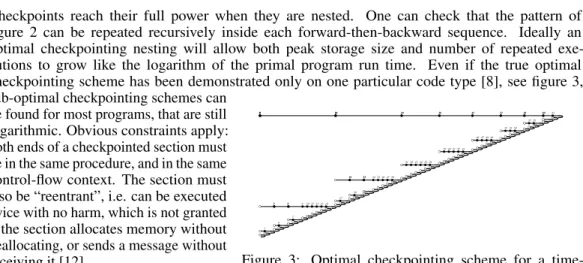
Checkpoints reach their full power when they are nested. One can check that the pattern of figure 2 can be repeated recursively inside each forward-then-backward sequence. Ideally an optimal checkpointing nesting will allow both peak storage size and number of repeated exe-cutions to grow like the logarithm of the primal program run time. Even if the true optimal checkpointing scheme has been demonstrated only on one particular code type [8], see figure 3,
0 56 6060 62 58 57 56 51 54 53 52 51 45 49 48 47 46 45 38 43 42 41 40 39 38 30 36 35 34 33 32 31 30 16 28 27 26 25 24 22 22 19 20 19 16 17 16 0 14 13 12 11 10 9 6 7 6 3 4 3 0 1 0
Figure 3: Optimal checkpointing scheme for a time-stepping loop of 64 steps: 9 snapshots, 3 repetitions sub-optimal checkpointing schemes can
be found for most programs, that are still logarithmic. Obvious constraints apply: both ends of a checkpointed section must be in the same procedure, and in the same control-flow context. The section must also be “reentrant”, i.e. can be executed twice with no harm, which is not granted if the section allocates memory without deallocating, or sends a message without receiving it [12]. . .
In practice, logarithmic growth is not
ex-actly what is desired. The available memory only allows for a fixed maximum number of snapshots q. It can be shown that the optimal checkpointing scheme then requires a number of repeated executions that grows like the q−th root of the primal program run time, which is still acceptable in general. In Tapenade, the default checkpointing scheme is to checkpoint each procedure call, except those non-reentrant. The user has freedom to deactivate checkpointing of desired calls, and to define additional checkpointed sections in the code.
4
Fixed-Point Iterations
Most code transformations can in general take advantage of additional semantic knowledge on parts of the code. This is true for adjoint AD in several situations such as parallel loops (gather-scatter), linear solvers. . . . We take here the example of Fixed-Point iterations. A Fixed-Point loop takes as input a state z and parameters x. At each iteration, z is recomputed as z = φ(z, x) until z converges up to some tolerance. The resulting, final z depends only on the parameters x. The input z is called the initial guess and only influences the iteration number till convergence. Adjoint AD must exploit
until z converges: z = φ(z, x) ... end z = φ(z, x) t = z until z converges: z = z ∂φ/∂z + t ... end x = x + z ∂φ/∂x
Figure 4: The Two-Phases adjoint of a Fixed-Point loop the fact that the initial
itera-tions operate on an arbitrary, al-most meaningless z, so that cor-responding intermediate values should not be stored. In fact, in the “Two-Phases” adjoint [3], see figure 4, only the intermediate values of the last, converged it-eration need be stored. On the other hand these intermediate val-ues will be used several times dur-ing the backward sweep. This re-quires a special stack mechanism for repeated access, which can be arranged easily.
Let’s conclude with an open question. When the Fixed-Point iteration is itself included in an iterative control, it is often profitable to reuse the previous Point as the initial guess of the next Fixed-Point iteration. This is called a warm start. Since the backward sweep of the adjoint code reproduces the same structure of nested iterative constructs, it should be possible to benefit also from a warm-start effect. However, strict application of the algorithm of figure 4 does not exhibit this effect. Only after a manual modification, poorly justified and unproved, could we retrieve a warm-start effect in the adjoint. This deserves further study.
References
[1] T. Albring, M. Sagebaum, and N.R. Gauger. Development of a consistent discrete adjoint solver in an evolving aerodynamic design framework. AIAA 2015-3240, 2015.
[2] A. Carle and M. Fagan. ADIFOR 3.0 overview. Technical Report CAAM-TR-00-02, Rice University, 2000.
[3] B. Christianson. Reverse accumulation and implicit functions. Optimization Methods and Software, 9(4):307–322, 1998.
[4] B. Dauvergne and L. Hascoët. The Data-Flow equations of checkpointing in reverse Automatic Differentiation. In International Conference on Computational Science, ICCS 2006, Reading, UK, 2006.
[5] M. Fagan, L. Hascoët, and J. Utke. Data representation alternatives in semantically aug-mented numerical models. In 6th IEEE International Workshop on Source Code Analysis and Manipulation, SCAM 2006, Philadelphia, PA, USA, 2006.
[6] R. Giering. Tangent linear and Adjoint Model Compiler, Users manual, 1997. http://www.autodiff.com/tamc.
[7] R. Giering and T. Kaminski. Generating recomputations in reverse mode AD. In G. Corliss, A. Griewank, C. Faure, L. Hascoët, and U. Naumann, editors, Automatic Differentiation of Algorithms: From Simulation to Optimization, chapter 33, pages 283–291. Springer Verlag, Heidelberg, 2002.
[8] A. Griewank. Achieving logarithmic growth of temporal and spatial complexity in reverse Automatic Differentiation. Optimization Methods and Software, 1:35–54, 1992.
[9] A. Griewank and A. Walther. Evaluating Derivatives: Principles and Techniques of Algorithmic Differentiation. Number 105 in Other Titles in Applied Mathematics. SIAM, Philadelphia, PA, 2nd edition, 2008.
[10] L. Hascoët, U. Naumann, and V. Pascual. TBR analysis in reverse mode Automatic Differen-tiation. Future Generation Computer Systems – Special Issue on Automatic Differentiation, 2004.
[11] L. Hascoët and V. Pascual. The Tapenade Automatic Differentiation tool: Principles, Model, and Specification. ACM Transactions On Mathematical Software, 39(3), 2013.
[12] L. Hascoët and J. Utke. Programming language features, usage patterns, and the efficiency of generated adjoint code. Optimization Methods and Software, 31:885 – 903, 2016.
[13] J. Lotz, K. Leppkes, and U. Naumann. dco/c++ - derivative code by overloading in C++. Technical report, Aachener Informatik-Berichte (AIB), 2011.
[14] U. Naumann. The Art of Differentiating Computer Programs: An Introduction to Algorithmic Differentiation. Number 24 in Software, Environments, and Tools. SIAM, Philadelphia, PA, 2012.
[15] J.M. Siskind and B.A. Pearlmutter. Efficient implementation of a higher-order language with built-in ad. In AD2016, Oxford, UK, 2016.
[16] J. Utke, U. Naumann, M. Fagan, N. Tallent, M. Strout, P. Heimbach, C. Hill, and C. Wunsch. OpenAD/F: A modular, open-source tool for Automatic Differentiation of Fortran codes. ACM Transactions on Mathematical Software, 34(4):18:1–18:36, 2008.
[17] A. Walther and A. Griewank. Getting started with ADOL-C. In Naumann and Schenk, editor, Combinatorial Scientific Computing, chapter 7, pages 181–202. Chapman-Hall CRC Computational Science, 2012.