HAL Id: hal-02933641
https://hal.inria.fr/hal-02933641
Submitted on 9 Sep 2020
HAL is a multi-disciplinary open access
archive for the deposit and dissemination of
sci-entific research documents, whether they are
pub-lished or not. The documents may come from
teaching and research institutions in France or
abroad, or from public or private research centers.
L’archive ouverte pluridisciplinaire HAL, est
destinée au dépôt et à la diffusion de documents
scientifiques de niveau recherche, publiés ou non,
émanant des établissements d’enseignement et de
recherche français ou étrangers, des laboratoires
publics ou privés.
Learning to plan with uncertain topological maps
Edward Beeching, Jilles Dibangoye, Olivier Simonin, Christian Wolf
To cite this version:
Edward Beeching, Jilles Dibangoye, Olivier Simonin, Christian Wolf. Learning to plan with uncertain
topological maps. ECCV 2020 - 16th European Conference on Computer Vision, Aug 2020, Glasgow,
United Kingdom. pp.1-24. �hal-02933641�
Edward Beeching1, Jilles Dibangoye1, Olivier Simonin1, and Christian Wolf2
1
INRIA Chroma team, CITI Lab. INSA Lyon, France. https://team.inria.fr/chroma/en/
2
Université de Lyon, INSA-Lyon, LIRIS, CNRS, France. {firstname.lastname}@insa-lyon.fr
Project page https://edbeeching.github.io/papers/learning_to_plan
Abstract. We train an agent to navigate in 3D environments using a hierarchical strategy including a high-level graph based planner and a local policy. Our main contribution is a data driven learning based approach for planning under uncertainty in topological maps, requiring an estimate of shortest paths in valued graphs with a probabilistic struc-ture. Whereas classical symbolic algorithms achieve optimal results on noise-less topologies, or optimal results in a probabilistic sense on graphs with probabilistic structure, we aim to show that machine learning can overcome missing information in the graph by taking into account rich high-dimensional node features, for instance visual information available at each location of the map. Compared to purely learned neural white box algorithms, we structure our neural model with an inductive bias for dynamic programming based shortest path algorithms, and we show that a particular parameterization of our neural model corresponds to the Bellman-Ford algorithm. By performing an empirical analysis of our method in simulated photo-realistic 3D environments, we demon-strate that the inclusion of visual features in the learned neural planner outperforms classical symbolic solutions for graph based planning.
Keywords: Visual navigation, topological maps, graph neural networks
1
Introduction
A critical part of intelligence is navigation, memory and planning. An animal that is able to store and recall pertinent information about their environment is likely to exceed the performance of an animal whose behavior is purely reactive. Many control and navigation problems in partially observed 3D environments involve long term dependencies and planning. It has been shown that humans and other animals navigate through the use of waypoints combined with a local locomotion policy [55,22]. In this work, we mimic this strategy by proposing a hierarchical planner, which performs high-level long term planning using an uncertain topological map (a valued graph including visual features) combined with a local RL-based policy navigating between high-level waypoints proposed by the graph planner. Our main contribution is a way to combine symbolic planning
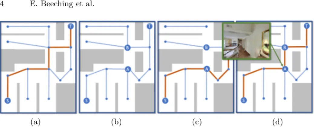
Fig. 1: A trained agent navigates to a goal location with a hierarchical planner. A high-level planner proposes new target nodes in a topological map (a graph), which are used as an objective for a local point-goal policy. The graph is estimated from an explorative rollout and, as such, uncertain: the opacities of the edges correspond to estimations of connectivity between nodes (darker lines = higher confidence). In this example we observe a low probability of connection between the node at the agent’s position (orange) and its nearest neighbor, whereas from the visual observation associated to the node we can see there is a traversable space between the two nodes.
with machine learning, and we look to structure a neural network architecture to incorporate landmark based planning in unseen 3D environments.
When solving visual navigation tasks, biological or artificial agents require an internal representation of the environment if they want to solve more complex tasks than random exploration. We target a scenario where an agent is trained on a large-scale set of 3D environments to learn to reason on planning and navigation. When faced with a previously unseen environment, the agent is given the opportunity to build a representation by doing an explorative rollout from a previously learned explorative policy. It can then exploit this internal representation in subsequent visual navigation tasks. This corresponds to many realistic situations, where robots are deployed to indoor environments and are allowed to familiarize themselves before performing their tasks [43].
Our agent constructs an imperfect topological map of its environment in the form of a graph, where nodes correspond to places and valued edges to connections. Edges are assigned two different values, the first one being spatial distances, the second one being probabilities indicating whether it is possible to navigate between the two nodes. Nodes are also assigned rich visual features extracted from images taken at the corresponding places in the environment. After deployment, the agent faces visual navigation tasks requiring it to find a specific location in the environment provided by a set of images corresponding
to different viewpoints, extending the task proposed in [63]. The objective is to identify the goal location in the internal representation, and to provide an estimate for the shortest path to it. The main difficulty we address here is the fact that this path is an estimate only, since the ground truth path is not available during testing / deployment.
Whilst planning in graphs with known connectivity has been solved for many decades [15,7], planning under uncertainty remains an ongoing area of research. Whereas optimal results in a probabilistic sense exist for graphs with probabilistic connectivity, we aim to show that machine learning can overcome missing information in the graph by taking into account rich high-dimensional node features, in particular features extracted from image observations associated with specific nodes. We train a graph neural network in a fully supervised way to predict estimates of the shortest path, using vision to overcome uncertainty in the connectivity information. We present a new variant of graph neural networks imbued with specific inductive bias, and we show that this structure can be parameterized to fallback to the classical Bellman-Ford algorithm.
Figure 1 illustrates the hierarchical planner: a neural graph based planner runs an outer loop providing estimates for next way-point on a graph, which are used as target nodes for a local RL-based policy running an inner loop and providing feedback to high-level planner on reached locations. Both planners take into account visual features, either stored in the graph (graph based planner), or directly as observations provided by the environment (local policy). The two planners are trained separately — the graph based planner in a fully supervised way from ground truth graphs, the local policy with RL and a point-goal strategy. This work makes the following contributions:
– A hierarchical model combining high-level graph based planning with a local point goal policy for robot navigation;
– A trainable high-level neural planner which combines an uncertain topological map (graph) with rich node features to learn to estimate shortest paths in noisy and unknown environments.
– A variant of graph networks encoding inductive bias inspired by dynamic programming-based shortest path algorithms.
– We evaluate the performance of the method in challenging and visually realistic 3D environments and show that it outperforms optimal symbolic planning on noisy topological maps.
2
Related work
Classical planning and graph search — A large body of work is available on classical planning on graphs, notable references include [31,42]. In robotics, there have been a number of works applying classical planning in topological maps for indoor robot navigation, for instance [48,54].
Planning under imperfect information — In many realistic robotic prob-lems, the current state of the world is unknown. Though sensor observations
(a) (b) (c) (d)
Fig. 2: Illustration of the different types of solutions to the high-level graph planning problem: (a) the ground truth graph (unavailable during testing) with the shortest path from node S to node T in red; (b) the uncertain graph available during test time. This graph is fully connected and for each edge a connection probability is available. For clarity we here show only edges where the connection probability is above a threshold. The edge from A→B is wrongly estimated as not connected; (c) an “optimal” path taking into account both probabilities and distances; (d) A learned shortest path, where the visual features at node A indicate passage to node B. We supervise a network to predict the GT path (a).
provide measurements about the current state of the world, these measurements are usually incomplete or noisy because of disturbances that distort their values. Planning problems that face these issues are referred to as planning problems under imperfect information. Research on this topic has a long history, which can be traced back to the seminal work by [2] presenting the first non-trivial exact dynamic programming algorithm for partially observable Markov decision processes (POMDPs). While there are other models [31, chap 12], POMDPs emerged as the standard framework to formalize and solve (single-agent) sequen-tial decision-making problems with imperfect information about the state of the world [26]. Since the agent does not have access to the actual state of the world, it acts based solely on its entire history of actions and observations, or the corresponding belief state, i.e., the posterior probability distribution over the states given the history [2,50]. Approaches for finding optimal solutions have been intensively investigated in the 2000s, ranging from dynamic programming [26] to heuristic search methods [51,30]. Key to these approaches is the idea that one can recast the original problem into a continuous-state fully observable Markov decision process, where states are belief states or histories [2]. Doing so allows theory and algorithm that applies for MDPs to also apply to POMDPs, albeit in much larger (and possibly continuous) state space. Another significant result of this literature is proof that the optimal value function is a piece-wise linear and convex function of the belief states, which allows the design of algorithms with faster rates of convergence [50]. For a thorough discussion on existing solvers for POMDPs, the reader can refer to [47].
Deep Reinforcement Learning — The field of Deep Reinforcement Learning (RL) has gained attention with successes on board games [49] and Atari games [37]. Recent works have applied Deep RL for the control of an agent in 3D environments [36] [24], exploring the use of auxiliary tasks such as depth predic-tion, loop detection and reward prediction to accelerate learning. Other recent work uses street-view scenes to train an agent to navigate in city environments [35]. To infer long term dependencies and store pertinent information about the partially observable environment, network architectures typically incorporate re-current memory such as Gated Rere-current Units [13] or Long Short-Term Memory [23]. Extensions to memory based neural approaches began with Neural Turing Machines [19] and Differentiable Neural Computers [20], and have since been adapted to expand the capacity of Deep RL agents [56]. Spatially structured memory architectures have been shown to augment an agent’s performance in 3D environments and are broadly split into two categories: metric maps which discretize the environment into a grid based structure and topological maps which produce node embeddings at key points in the environment. Research in learning to use a metric map is extensive and includes spatially structured memory [40], Neural SLAM based approaches [61] and approaches incorporating projective geometry and neural memory [21,8], these techniques are combined, extended and evaluated in [6]. Other notable works in include that of Value Iteration Networks (VIN) [53] which approximate the value iteration algorithm with a CNN, applied planning in small fully observable state spaces (grid worlds). While VIN and our work structure planners, VINs use convolutions to approximate classical value iteration, while we use a graph representation and a novel GNN architecture with recurrent updates to approximate the Bellman-Ford algorithm. [27] plans under uncertainty in partially observable gridworld environments. Here uncertainty refers to POMPs, the classical QMDP algorithm is used as inductive bias for a neural network, whereas in our work uncertainty is over node connectivity in a graph constructed in a previously unseen environment. [52] which is applied in observable state spaces to learn a forward model in a latent space to plan appropriate actions; they are not hierarchical, are not graph-based and do not appear to plan under uncertainty. Similar to ours, they are applied to goal driven problems.
Research combining learning, navigation in 3D environments and topological representations has been limited in recent years with notable works being [43] who create graph a through random exploration in ViZDoom RL environment [28]. [16] also performs planning in 3D environments on a graph-based structure created from randomly sampled observations, with node distances estimated with value estimates. The downside of these approaches is that in order to generalize to an unseen environment, many random samples must be taken in order to populate the graph.
Graph neural networks — Graph Neural Networks (GNN) are deep networks that operate on graphs directly. They have recently shown great promise in domains such as knowledge graphs [44], chemical analysis [18], protein interac-tions [17], physics simulainterac-tions [3] and social network analysis [29]. These types
of architectures enable learning from both node features and graph connectiv-ity. Several review papers have covered graph neural networks in great detail [9,4,57,62]. GNNs have been applied to shortest path planning in travelling salesmen problems [33,25] and it has been reasoned that they can approximate optimal symbolic planning algorithms such as the Bellman-Ford algorithm [60]. This work applies a novel variant of GNN in order to solve approximate planning problems, where classical methods may struggle to deal with uncertainty.
3
Hierarchical navigation with uncertain graphs
We train an agent to navigate in a 3D visual environment and to exploit an internal representation, which it is allowed to obtain from an explorative rollout before the episode. Our objective is image goal, i.e. target-driven navigation to a location which is provided through a (visual) image. We extend the task introduced in [63] by generalizing to unseen environment configurations without the need to retrain the agent for a novel environment.
From the explorative rollout obtained with an agent trained with RL, which is further described in section 3.3, we create an uncertain topological map covering the environment, i.e. a valued graph G={V, V , E, L, D}, where V={1, . . . N } is a set of nodes, V is a K×N matrix of rich visual node features of dimensions
K, E ∈ [0, 1]N ×N is a set of edge probabilities where Ei,j is the probability of
having an edge between nodes i and j, L is a matrix of node locations and D is a
distance matrix, where Di,j is a distance between nodes i and j. While D encodes
a distance in a path planning sense, E encodes the probability of j being directly accessible from i with obstructions. The uncertainty encoded by this probability can be considered to be a combination of aleatory variability, i.e. uncertainty associated with natural randomness of the environment, as well as epistemic uncertainty, i.e. uncertainty associated with variability in computational models for estimating the graph, in our case the explorative policy trained with RL and taking into account visual observations.
Once the topological map is obtained, the objective of the agent at each episode is to navigate to a location given an image, which is provided as additional observation at each time step. The agent acts in 3D environments like Habitat[34] (see section 5), receiving images of the environment as observations and predicting actions from a discrete space (forward, turn left 10◦, turn right 10◦). We propose a hierarchical planner performing actions at two different levels:
A high-level graph based planner that operates on longer time scale τ and
iteratively proposes new point-goals nodes pτ
g that are predicted, by a Graph
Neural Network, to be on the shortest path from the agent to the estimated location of the target image.
A local policy that has been trained to navigate to a local point-goal pτ
g, which
has been provided by the high-level policy. The local policy operates for a maximum of m time-steps, where m is a hyper-parameter, set to 10. The agent has been trained with an additional STOP action, so that it can learn
to terminate the local policy in the case that it reaches pτ
The two planners communicate through estimated locations, the graph planner indicating the next waypoint to the local policy as a location, and the local policy (after termination) providing an estimate of its reached location back to the high-level planner. The planner updates its current node estimate as the nearest neighboring node and planning continues.
3.1 High-level planning with uncertain graphs
The objective of the high-level planner is to estimate the shortest path from the current position S∈V in the graph to a terminal node T ∈V, whose identity is estimated as the node whose visual features are closest to the target image in cosine distance. Planning takes into account the distances between nodes encoded in D as well as estimated edge connectivity encoded in E. As an edge (i, j)
may have a large connection probability Ei,j but still be obstructed in reality,
the goal is to learn a trainable planner parameterized by parameters θ, which takes into account visual features V to overcome the uncertainty in the graph
connectivity. To this end, we assume the ground truth connectivity E∗ available
during training only. Figure 2 illustrates the different types of solutions this problem admits: the optimal shortest path is only available on ground truth data (Figure 2a), the objective is to use the noisy uncertain graph (Figure 2b) and provide an estimate of the optimal solution taking into account visual features (Figure 2d). This is unlike the optimal solution in a probabilistic sense calculated
from a symbolic algorithm (Figure 2c).
We propose a trainable planner, which consists of a novel graph neural network architecture with dedicated inductive bias for planning. Akin to graph networks [5], the node embeddings are updated with messages over the edges, which propagate information over the full graph. While it has been shown that graph networks can be trained to perform planning [59], we aim to closely mimic the structure of the Bellman-Ford algorithm and we embue the planner with additional inductive bias and a supervised objective to explicitly learn to calculate shortest paths from data. To this end, each node i of the graph is assigned an embedding xi= [vi, ei, ti, di, si] where vi are visual features from the memory
matrix V , ti is a boolean value indicating if the node is the target, ei are the
edge connection probabilities from node i to all other nodes, diare the distances
for node i to all other nodes, si is a one hot vector identifying the node (part of
the identity matrix I).
We motivate our proposed neural model with the following objective: the planner should be able to exploit information contained in the graph connectivity, but also in the visual features, to be able to find the shortest path from a given current node to a given target node. As with classical planning algorithms, it will thus eventually be required to keep for each node a latent representation of
the bound di on the shortest distance as well as information on the identity of
the outgoing edge to the neighbor lying on the shortest path, the predecessor function Π(i). Known algorithms (Dijstra, Bellman-Ford) perform iterative
updates of these variables (di, Πi) by comparing them with neighboring nodes
a shorter path is found than the current one. This is usually done by iterating over the successors of a given node i.
In our trained model, these variables are not made explicit, but they are supposed to be learned as a unique vectorial latent representation for each node
i in the form of an internal state ri, which generally holds current information
on the reasoning of the agent. The input to each iteration of the graph network
is, for each node i, the node embedding xi, and the node state ri, which we
concatenate to form a single node vector ni:
ni= [xi, ri] = [vi, ei, ti, di, si, ri]
As classically done in graph neural networks, this representation is updated iteratively by exchanging messages between nodes in the form of trainable functions. The messages and trainable functions of our model are given as follows, illustrated in Figure 3, and will be motivated in detail further below.
mi,j= W1[ni, nj] σ(W2[ni, nj]) (1)
r0i= φr←h({mi,j}∀j, hi) (2)
Here, is the Hadamard product, W.are weight matrices, and ri0is the updated
latent representation after one round of updates. The features xi do not change
during these operations.
Equation (1) is inspired from gated linear layers [14], and enables each node to identify whether it is the target, and update its representation of the bound. We use gated linear layers in order to provide the network with the capacity to update bound estimates for its neighbors.
Equation (2) integrates messages from all neighbors j of node i, updating its latent representation. Since planning requires this step to update internal bounds on shortest paths, akin to shortest path algorithms that rely on dynamic programming, we serialize the updates from different neighbors into a sequence of updates, which allows the network to learn to calculate minimum functions on bound estimates. In particular, we model this through a recurrent network in a
Gated Recurrent Unit variant [12], using a hidden state vector hi associated to
each node i. The step is structured to mimic the min operation of the Bellman-Ford algorithm (see section 3.2 for details on this equivalence).
Equation (2) can thus be rewritten in more detail as follows: Going sequentially
over the different neighbors j of node i, the hidden state hiis updated as follows:
h[j]i = W3mi,j+ W4h [j−1]
i (3)
For simplicity, we omitted the gating equations of GRUs and presented a single layer GRU. In practice we include all gating operations and use a stacked GRU with two layers. The output of the recurrent unit is a non-linear function of the last hidden state, providing the new latent value ri0:
r0i= M LP (hNi ) (4)
(a) (b)
Fig. 3: (a) An example graph; (b) One iteration of the neural graph planner’s message passing and bound update. Incoming messages from neighbors are serialized and fed through a recurrent unit, which creates inductive bias for learning minima necessary for bound updates.
The above messages are exchanged and accumulated for k steps where k is a hyper-parameter which should be at least the largest span of the graphs in
the dataset. The action distribution fA(ri) is then estimated for each node in
the graph as a linear mapping of the node embeddings followed by a softmax activation function.
Ai= fA(ri) = softmax(W ri) (5)
3.2 Relations to optimal symbolic planners
As mentioned before, our neural planner could in theory be instantiated with a specific set of network parameters such that it corresponds to a known sym-bolic planner calculating an optimal path in a certain sense. To illustrate the relationship of the network structure, in particular the recurrent nature of the graph updates, we will layout details for the case where the planner performs the estimation of a shortest path given the distance matrix and ignoring the uncer-tainty information — an adaptation to an optimal planner in the probabilistic sense can be done in a straightforward manner. To avoid misunderstandings, we insist that the reasoning developed in this sub section is for illustration and general understanding of the chosen inductive network bias only, the real network parameters are fully trained with supervised learning as explained in section 4. Handcrafting a parameterization requires imposing a structure on the node
state ri, which otherwise is a learned representation. In our case, the node state
will be composed of the bound bion the shortest path from the given node to the
target node (a scalar), and the current estimate Πi of the identity of predecessor
node of node i w.r.t. the shortest path, which can be represented as a 1-in-K encoded vector indicating a distribution over nodes.
Standard Bellman-Ford symbolic bound updates iteratively update the bound for a given node i by examining all its neighbors j and checking whether a shorter
path can be found passing through neighbor j. This can be written in a sequential
form s.t. the bound gets updated iterating through the neighbors j=1. . .Ji of
node i: b[0]i = bi b[j]i = min(b[j−1]i , bj+ dij) b0i = b[Ji] i (6)
where bi is the bound before the round of updates for node i, and b0iis the bound
after the round of updates for node i.
In our neural formulation, the message updates given in equation (2), further developed in (3), mimic the Bellman-Ford bound update given in Equations (6). This provided motivation for our choice of a recurrent neural network in
the graph neural network, as we require the update of the recurrent state hji
in Equation (3) to be able to perform a minimum operation and an arg min operation (or differentiable approximations of min and arg min).
3.3 Graph creation from explorative rollouts
Graphs were generated during the initial rollout from an exploratory policy trained with Reinforcement Learning. During training, the agent interacts with training environments and receives RGB-D image observations calculated as a projection from the 3D environment. The agent is trained to explore the environment and to maximize coverage, i.e. to visit as much space as possible as quickly as possible similar to [10,11].
To learn to estimate the graph connectivity, we add an auxiliary loss to the agent’s objective function, flink(oi, oj, hi) which is trained to classify whether
two locations are in line of sight of each other, conditioned on the visual features
oi, oj from the two locations and the agent’s hidden state hi. Node features
were calculated with a CNN [32]. Ground truth line of sight measurements were computed by 2D ray tracing on an occupancy map of each environment. In order to limit the size of the graph to a maximum number of nodes k, we aim to maximize each node’s coverage of the environment using a Gaussian kernel function. At each time step a new node is observed by the agent, previous node positions are compared with a Gaussian kernel function (eq. 7) in order to identify the index of the most redundant node r, which is removed from the graph and replaced with the new node, node connectivities are then recomputed with flink(.), where Li is the location of node i.
r = arg min i X j K(Li, Lj) , K(v, v 0) = exp(−kv − v0k2 2σ2 ), (7)
4
Training
The high-level graph based planner — is trained in a purely supervised way. We generate ground truth labels by running a symbolic algorithm (Dijkstra [15])
on a set of valued ground truth training graphs described with the method detailed in Section 3.3. In particular, the supervised training algorithm takes as input uncertain/noisy graphs, which include visual features, and is supervised to learn to produce paths, which are calculated from known ground truth graphs unavailable during test time. During training we treat path planning as a classification problem where for a given target, each node must learn to predict the subsequent node on the optimal path to the target.
Formally for each node i we predict a distribution Ai and aim to match a
ground-truth distribution A∗
i, which is a one-hot vector, minimizing cross entropy
loss L(A, A∗) = −Pn
i=1A
∗ ilog Ai.
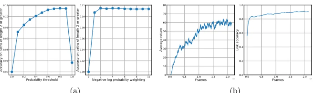
We augment training with a novel version of mod-drop [39], a training al-gorithm for multi-modal data, which drops modalities probabilistically during training. In our case, during training we extend the node connection proba-bilities in the input with the ground truth node adjacencies and mask either the probabilities or the adjacencies with a probability of 50%, during training we linearly taper the masking probability from 50% to 100% over the first 250 epochs. This ensures that the final model requires only connection probabilities, but the reasoning performed during message passing and recurrent updates can be bootstrapped from the ground truth adjacency matrix. Training curves on unseen validation data are shown in figure 5b.
The local policy — is a recurrent version of AtariNet [38] with two output heads for the action distribution and value estimates. The network was trained with a reinforcement learning algorithm Proximal Policy Optimization (PPO) [45] to navigate with discrete actions to a local point-goal. Point-goals were generated to be within 5m of the spawn location of agent. A dense reward was provided that corresponds to a decrease in geodesic distance to the target, a large reward (10.0) was provided when the agent reached the target and the STOP action was used. The episode was terminated when either the STOP action was used or after 500 time-steps. A small negative reward of -0.01 was given at each time-step to encourage the agent to complete the task quickly.
The explorative policy for graph creation — is trained with PPO [46]. We aim to maximize coverage that is within the field of view of the agent. We create an occupancy grid of the environment with a grid spacing of 10cm. The first time a cell is observed the agent receives a reward of 0.1. A cell is considered to observable if it is free space, within 3m of the agent and in the field of view of the agent. Agent performance is shown in Figure 4b.
5
Experiments
We evaluated our method in simulated 3D environments, in particular the Habitat [34] simulator with the visually realistic Gibson dataset [58]. During training, the agent interacts with 72 different training environments from Gibson, where each environment corresponds to a different apartment or house, and receives as input observation an observed RGB-D image. We evaluate our method on a set
0.0 0.2 0.4 0.6 0.8 1.0 Probabilty threshold 0.00 0.02 0.04 0.06 0.08 0.10 0.12
Accuracy on paths of length 2 or greater
0 2 4 6 8 10
Negative log probabilty weighting
0.00 0.02 0.04 0.06 0.08 0.10 0.12
Accuracy on paths of length 2 or greater
(a) 0.0 0.5 1.0 1.5 2.0 Frames 1e8 0 10 20 30 40 50 60 70 80 Average return 0.0 0.5 1.0 1.5 2.0 Frames 1e8 0.0 0.2 0.4 0.6 0.8 1.0 Link accuracy (b)
Fig. 4: (a) Symbolic baselines Dijkstra on - left: thresholded probs., right: cost function(8). (b) Left: Average return. Right: Accuracy of line of sight predictions. Table 1: Reporting H-SPL and accuracy of the neural planner’s predictions in unseen environments; neural planner trained with 72,000 graphs
(a) Results on uncertain graphs
Method Acc H-SPL
Symbolic (threshold) 0.114 0.184
Symbolic (custom cost) 0.115 0.269
Neural (w/o visual) 0.251 0.468
Neural (w visual) 0.262 0.501
(b) Results on ground truth graphs
Method Acc H-SPL
Symbolic (GT) 1.00 1.00
Neural planner (GT) 0.921 0.983
of 16 held out environments that were unseen during training by either the local policy, the exploratory policy or the high-level neural planner.
5.1 High-level graph-based planner
The neural planner was implemented in PyTorch [41], the hyper-parameters are given in the supplementary material. We compare two metrics, accuracy of prediction of the next way-point along the optimal path and the SPL metric [1], both for paths of length two or greater. As we evaluate SPL for both the high level planner and the hierarchical planner-controller, we refer to the high-level planner’s SPL as H-SPL to avoid ambiguity.
Symbolic baselines — We compare the neural planner to two symbolic base-lines, both of which reason on the uncertain graph only, without taking into account rich node features. While these baselines are “optimal” with respect to their respective objective functions, they are optimal with respect to the amount of information available to them, which is uncertain: (i) Thresholding — In order to generate non-probabilistic edge connections, we threshold the connection probabilities with values ranging from 0-1 in steps of 0.1. After threshholding the graph, path planning was performed with Dijkstra’s algorithm; (ii) A custom cost function for Dijkstra’s algorithm weighting distances and probabilities:
10000 20000 30000 40000 50000 60000 70000
Training dataset size
0.12 0.14 0.16 0.18 0.20 0.22 0.24 0.26 Validation accuracy Connection probabilities Probabilities and visual features
10000 20000 30000 40000 50000 60000 70000
Training dataset size
0.300 0.325 0.350 0.375 0.400 0.425 0.450 0.475 0.500 Validation H-SPL Connection probabilities Probabilities and visual features
(a) 0 50 100 150 200 250 300 Training epochs 0.05 0.10 0.15 0.20 0.25 0.30 0.35
Accuracy on paths of length 2 or greater No modality mixingModality mixing for first 250 epochs
(b)
Fig. 5: (a) Accuracy and H-SPL with increasing size of data when the GNN is trained with and without visual features. (b) Modality mixing (GT connections and probabilities), we observe a 2.3% improvement over single modality training.
We vary the weighting λ in order to control the trade-off of distance and connection probability. In the limit where λ is 0, the graph is a fully connected graph, whereas high values of λ would lead to finding the most probable path.
Results of both symbolic baselines for varying hyper-parameters are shown in Figure 4a, we observe that they perform poorly under uncertainty. In both cases we aim to evaluate the accuracy of their predictions with respect to the symbolic baseline on the ground truth graph, i.e. Dijkstra on the shortest path. As graphs can contain many source-target pairs that are within 1 step, we report accuracy on source-target pairs separated by at least 2 steps.
Image driven recurrent baseline — We also compare to an end-to-end RL approach where the current observation and target image are provided to a CNN based RL agent trained from reward. The agent architecture is a siamese CNN with a recurrent GRU. We train with a dense reward of improvement in geodesic distance between the agent and the target, and provide a reward of 10 when the agent reaches the goal. We used PPO, and trained for 200 M environment frames.
In Table 1a, we compare the neural planner,the two symbolic baselines and the recurrent baseline. We can see, that even without visual features, the neural planner is able to outperform the “optimal” symbolic baselines. This can be explained with the fact, that the baselines optimize a fixed criterion, whereas the neural planner can learn to exploit patterns in the connection probability matrix E to infer valuable information on shortest ground truth path. The gap further increases when the neural planner can use visual features. The positive impact of modality mixing (see section 4) is shown in Figure 5b.
As a sanity check, table 1b compares the optimal symbolic planner against the neural planner trained with ground truth adjacencies provided as input. We observe that the results of the neural planner are close to optimum in this case. We evaluated our approach with different amounts of training data, ranging from 8,000 graphs to 74,000 training graphs (Figure 5a). Note that one training
Time-step 10 Time-step 20 Time-step 30
Time-step 65 Time-step 55
Time-step 40
Fig. 6: Six time-steps from a rollout of the hierarchical planner (graph+local) in an unseen testing environment. For each time-step: left – RGB-D observation, right
– map of the environment (unseen) withgraph nodes, source node,target node,
agent position(black),nearest neighbourto the agent, local point-goalprovided
by the high level planner and planned path. Further examples can be found in
the supplementary material, including failure cases.
graph spawns 32×32 possible source-target combinations, leading to a maximum amount of 75,000,000 training instances.
5.2 Hierarchical planning and control (topological & local policy)
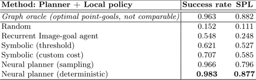
We evaluated the neural graph planner coupled with the local policy. For a given episode, the graph planner estimates the next node in the path to a target image and provides its location to the local policy, which executes for m time-steps. The planner then re-plans from the nearest neighbor to the agent’s current position, this back and forth process of planning and navigating continues until either the agent reaches the target or 500 low-level time-steps have been conducted. We report accuracy as percentage of runs completed successfully and SPL in table 2, albeit measured on low-level trajectories as opposed to graph space. We combine the local policy with various graph planners, and can see that the neural graph planners greatly outperform the symbolic baselines. We perform two evaluations of the neural planner; a deterministic evaluation where point-goals are chosen with the argmax of the A distribution and a non-deterministic one by sampling from A. The motivation is that by sampling, the planner can escape from local minima and loops created by errors in approximation. This is confirmed when studying rollouts from the agents, and also quantitatively through the performances shown
Table 2: Performance of the hierarchical graph planner & local policy
Method: Planner + Local policy Success rate SPL
Graph oracle (optimal point-goals, not comparable) 0.963 0.882
Random 0.152 0.111
Recurrent Image-goal agent 0.548 0.248
Symbolic (threshold) 0.621 0.527
Symbolic (custom cost) 0.707 0.585
Neural planner (sampling) 0.966 0.796
Neural planner (deterministic) 0.983 0.877
in table 2. A visualization of steps from an episode is shown in Figure 6, where in step 10 we can see that navigation is robust w.r.t. local errors in planning (the purple line crossing white non-traversable space).
5.3 Ablation: Effect of chosen inductive bias
As developed in sections 3.1 and 3.2, our graph based planner includes a particular inductive bias, which allows it to represent the Bellman-Ford algorithm for the calculation of shortest or best paths. This bias is implemented as a recurrent model (a GRU) running sequentially over the message passing procedures, as illustrated in Figure 3.
Figure 7 ablates the effect of this additional bias as a function of data sizes
ranging from 8,000 to 74,000 example graphs, each one evaluated with 322=1,024
different combinations of starting and end points.
The differences are substantial, and we can see that our model is able to exploit increasing amounts of data and translates them into gains in performance, whereas standard graph convolutional networks don’t — we conjecture that they lack in structure allowing them to pick up the required reasoning.
6
Conclusion
We demonstrated that path planning algorithms can be approximated with learning when structured in a manner that is akin to classical path planning algorithms. We have performed an empirical analysis of the proposed solution in photo-realistic 3D environments and have shown that in uncertain environments graph neural networks can outperform their symbolic counterparts by incorpo-rating rich visual features as part of their planning procedure. Our method can be used to augment a vision based agent with the ability to form long term plans under uncertainty in novel environments, without a priori knowledge of the particular environment. We have analysed the empirical performance of the neural planning algorithm with a variety of dataset sizes, shown that the high-level planner can be coupled with a low-level policy and evaluated the hierarchical performance on an image-goal task.
20000 40000 60000 Dataset size 0.075 0.100 0.125 0.150 0.175 0.200 0.225 0.250
Accuracy on paths of length 2 or greater Ablation: no GRU for min operationAblation: GRU for min operation
20000 40000 60000 Dataset size 0.20 0.25 0.30 0.35 0.40 0.45
H-SPL on paths of length 2 or greater Ablation: no GRU for min operation
Ablation: GRU for min operation
Fig. 7: Ablation of the addition of a GRU for the accumulation of incoming messages. This recurrent unit was added to ensure that the model could represent the Bellman-Ford algorithm.
Acknowledgements — This work was funded by grant Deepvision (ANR-15-CE23-0029, STPGP479356-15), a joint French/Canadian call by ANR & NSERC; Compute was provided by the CNRS/IN2P3 Computing Center (Lyon, France), and by GENCI-IDRIS (Grant 2019-100964).
References
1. Anderson, P., Chang, A., Chaplot, D.S., Dosovitskiy, A., Gupta, S., Koltun, V., Kosecka, J., Malik, J., Mottaghi, R., Savva, M., Zamir, A.R.: On evaluation of embodied navigation agents (2018)
2. Åström, K.J.: Optimal control of markov processes with incomplete state informa-tion. Journal of Mathematical Analysis and Applications 10(1), 174–205 (1965) 3. Battaglia, P., Pascanu, R., Lai, M., Rezende, D.J., et al.: Interaction networks for
learning about objects, relations and physics. In: Advances in neural information processing systems. pp. 4502–4510 (2016)
4. Battaglia, P.W., Hamrick, J.B., Bapst, V., Sanchez-Gonzalez, A., Zambaldi, V., Ma-linowski, M., Tacchetti, A., Raposo, D., Santoro, A., Faulkner, R., et al.: Relational inductive biases, deep learning, and graph networks. arXiv preprint arXiv:1806.01261 (2018)
5. Battaglia, P., Hamrick, J., Bapst, V., Sanchez-Gonzalez, A., Zambaldi, V., Mali-nowski, M., Tacchetti, A., Raposo, D., Santoro, A., Faulkner, R., Gülçehre, Ç., Song, F., Ballard, A., Gilmer, J., Dahl, G., Vaswani, A., Allen, K., Nash, C., Langston, V., Dyer, C., Heess, N., Wierstra, D., Kohli, P., Botvinick, M., Vinyals, O., Li, Y., Pascanu, R.: Relational inductive biases, deep learning, and graph networks. arXiv preprint 1807.09244 (2018)
6. Beeching, E., Wolf, C., Dibangoye, J., Simonin, O.: Egomap: Projective mapping and structured egocentric memory for deep rl (2020)
7. Bellman, R.: On a routing problem. Quarterly of applied mathematics 16(1), 87–90 (1958)
8. Bhatti, S., Desmaison, A., Miksik, O., Nardelli, N., Siddharth, N., Torr, P.H.S.: Playing doom with slam-augmented deep reinforcement learning. arxiv preprint 1612.00380 (2016)
9. Bronstein, M.M., Bruna, J., LeCun, Y., Szlam, A., Vandergheynst, P.: Geometric deep learning: going beyond euclidean data. IEEE Signal Processing Magazine 34(4), 18–42 (2017)
10. Chaplot, D.S., Gandhi, D., Gupta, S., Gupta, A., Salakhutdinov, R.: Learning to explore using active neural slam. In: International Conference on Learning Representations (2020), https://openreview.net/forum?id=HklXn1BKDH
11. Chen, T., Gupta, S., Gupta, A.: Learning exploration policies for navigation. In: International Conference on Learning Representations (2019), https://openreview. net/forum?id=SyMWn05F7
12. Chung, J., Gulcehre, C., Cho, K., Bengio, Y.: Empirical evaluation of gated recurrent neural networks on sequence modeling. arXiv preprint arXiv:1412.3555 (2014) 13. Chung, J., Gulcehre, C., Cho, K., Bengio, Y.: Gated Feedback Recurrent Neural
Networks. In: ICML (2015)
14. Dauphin, Y.N., Fan, A., Auli, M., Grangier, D.: Language modeling with gated convolutional networks. In: Proceedings of the 34th International Conference on Machine Learning-Volume 70. pp. 933–941. JMLR. org (2017)
15. Dijkstra, E.W.: A note on two problems in connexion with graphs. Numerische mathematik 1(1), 269–271 (1959)
16. Eysenbach, B., Salakhutdinov, R.R., Levine, S.: Search on the replay buffer: Bridging planning and reinforcement learning. In: Advances in Neural Information Processing Systems 32, pp. 15220–15231. Curran Associates, Inc. (2019)
17. Fout, A., Byrd, J., Shariat, B., Ben-Hur, A.: Protein interface prediction using graph convolutional networks. In: Advances in neural information processing systems. pp. 6530–6539 (2017)
18. Gilmer, J., Schoenholz, S.S., Riley, P.F., Vinyals, O., Dahl, G.E.: Neural message passing for quantum chemistry. In: Proceedings of the 34th International Conference on Machine Learning-Volume 70. pp. 1263–1272. JMLR. org (2017)
19. Graves, A., Wayne, G., Danihelka, I.: Neural turing machines. arXiv preprint arXiv:1410.5401 (2014)
20. Graves, A., Wayne, G., Reynolds, M., Harley, T., Danihelka, I., Grabska-Barwińska, A., Colmenarejo, S.G., Grefenstette, E., Ramalho, T., Agapiou, J., et al.: Hy-brid computing using a neural network with dynamic external memory. Nature 538(7626), 471 (2016)
21. Gupta, S., Davidson, J., Levine, S., Sukthankar, R., Malik, J.: Cognitive map-ping and planning for visual navigation. In: 2017 IEEE Conference on Com-puter Vision and Pattern Recognition (CVPR). pp. 7272–7281 (July 2017). https://doi.org/10.1109/CVPR.2017.769
22. Gupta, S., Fouhey, D., Levine, S., Malik, J.: Unifying map and landmark based representations for visual navigation. arXiv preprint arXiv:1712.08125 (2017) 23. Hochreiter, S., Schmidhuber, J.: Long Short-Term Memory. Neural Computation
9(8), 1735–1780 (1997)
24. Jaderberg, M., Mnih, V., Czarnecki, W.M., Schaul, T., Leibo, J.Z., Silver, D., Kavukcuoglu, K.: Reinforcement learning with unsupervised auxiliary tasks. In: ICLR (2017)
25. Joshi, C.K., Laurent, T., Bresson, X.: An efficient graph convolutional network technique for the travelling salesman problem. arXiv preprint arXiv:1906.01227 (2019)
26. Kaelbling, L.P., Littman, M.L., Cassandra, A.R.: Planning and acting in partially observable stochastic domains. Artificial intelligence 101(1-2), 99–134 (1998) 27. Karkus, P., Hsu, D., Lee, W.S.: Qmdp-net: Deep learning for planning under partial
observability (2017)
28. Kempka, M., Wydmuch, M., Runc, G., Toczek, J., Jaskowski, W.: ViZ-Doom: A Doom-based AI research platform for visual reinforcement learn-ing. IEEE Conference on Computatonal Intelligence and Games, CIG (2017). https://doi.org/10.1109/CIG.2016.7860433, https://arxiv.org/pdf/1605.02097. pdf
29. Kipf, T.N., Welling, M.: Semi-supervised classification with graph convolutional networks. In: International Conference on Learning Representations (2017) 30. KURNIAWATI, H.: Sarsop: Efficient point-based pomdp planning by approximating
optimally reachable belief spaces. Proc. Robotics: Science and Systems, 2008 (2008) 31. LaValle, S.M.: Planning algorithms. Cambridge university press (2006)
32. Lecun, Y., Eon Bottou, L., Bengio, Y., Haaner, P.: Gradient-Based Learning Applied to Document Recognition. Proceedings of the IEEE 86(11), 2278 – 2324 (1998) 33. Li, Z., Chen, Q., Koltun, V.: Combinatorial optimization with graph convolutional
networks and guided tree search. In: Advances in Neural Information Processing Systems. pp. 539–548 (2018)
34. Manolis Savva*, Abhishek Kadian*, Oleksandr Maksymets*, Zhao, Y., Wijmans, E., Jain, B., Straub, J., Liu, J., Koltun, V., Malik, J., Parikh, D., Batra, D.: Habitat: A Platform for Embodied AI Research. In: Proceedings of the IEEE/CVF International Conference on Computer Vision (ICCV) (2019)
35. Mirowski, P., Grimes, M.K., Malinowski, M., Hermann, K.M., Anderson, K., Teplyashin, D., Simonyan, K., Kavukcuoglu, K., Zisserman, A., Hadsell, R.: Learning to Navigate in Cities Without a Map. arxiv pre-print 1804.00168v2 (2018) 36. Mirowski, P., Pascanu, R., Viola, F., Soyer, H., Ballard, A.J., Banino, A., Denil,
M., Goroshin, R., Sifre, L., Kavukcuoglu, K., Kumaran, D., Hadsell, R.: Learning to Navigate in Complex Environments. In: ICLR (2017)
37. Mnih, V., Kavukcuoglu, K., Silver, D., Rusu, A.A., Veness, J., Bellemare, M.G., Graves, A., Riedmiller, M., Fidjeland, A.K., Ostrovski, G., Petersen, S., Beattie, C., Sadik, A., Antonoglou, I., King, H., Kumaran, D., Wierstra, D., Legg, S., Hassabis, D.: Human-level control through deep reinforcement learning. Nature 518(7540) (2015)
38. Mnih, V., Kavukcuoglu, K., Silver, D., Rusu, A.A., Veness, J., Bellemare, M.G., Graves, A., Riedmiller, M., Fidjeland, A.K., Ostrovski, G., Petersen, S., Beattie, C., Sadik, A., Antonoglou, I., King, H., Kumaran, D., Wierstra, D., Legg, S., Hassabis, D.: Human-level control through deep reinforcement learning. Nature 518 (2015). https://doi.org/10.1038/nature14236, https://storage.googleapis. com/deepmind-media/dqn/DQNNaturePaper.pdf
39. Neverova, N., Wolf, C., Taylor, G., Nebout, F.: Moddrop: adaptive multi-modal ges-ture recognition. IEEE Transactions on Pattern Analysis and Machine Intelligence 38(8), 1692–1706 (2015)
40. Parisotto, E., Salakhutdinov, R.: Neural map: Structured memory for deep rein-forcement learning. In: ICLR (2018)
41. Paszke, A., Gross, S., Massa, F., Lerer, A., Bradbury, J., Chanan, G., Killeen, T., Lin, Z., Gimelshein, N., Antiga, L., Desmaison, A., Kopf, A., Yang, E., DeVito, Z., Raison, M., Tejani, A., Chilamkurthy, S., Steiner, B., Fang, L., Bai, J., Chintala, S.: Pytorch: An imperative style, high-performance deep learning library. In: Wallach, H., Larochelle, H., Beygelzimer, A., d’Alché Buc, F., Fox, E., Garnett, R. (eds.)
Advances in Neural Information Processing Systems 32, pp. 8024–8035. Curran Associates, Inc. (2019)
42. Remolina, E., Kuipers, B.: Towards a general theory of topological maps. Artif. Intell. 152, 47–104 (2004)
43. Savinov, N., Dosovitskiy, A., Koltun, V.: Semi-parametric topological memory for navigation. In: International Conference on Learning Representations (2018), https://openreview.net/forum?id=SygwwGbRW
44. Schlichtkrull, M., Kipf, T.N., Bloem, P., Van Den Berg, R., Titov, I., Welling, M.: Modeling relational data with graph convolutional networks. In: European Semantic Web Conference. pp. 593–607. Springer (2018)
45. Schulman, J., Wolski, F., Dhariwal, P., Radford, A., Klimov, O.: Proximal policy optimization algorithms. arxiv pre-print 1707.06347 (2017)
46. Schulman, J., Wolski, F., Dhariwal, P., Radford, A., Klimov, O.: Proximal policy optimization algorithms. arXiv preprint arXiv:1707.06347 (2017)
47. Shani, G., Pineau, J., Kaplow, R.: A survey of point-based pomdp solvers. Au-tonomous Agents and Multi-Agent Systems 27(1), 1–51 (2013)
48. Shatkay, H., Kaelbling, L.P.: Learning topological maps with weak local odometric information. In: IJCAI (2). pp. 920–929 (1997)
49. Silver, D., Hubert, T., Schrittwieser, J., Antonoglou, I., Lai, M., Guez, A., Lanctot, M., Sifre, L., Kumaran, D., Graepel, T., Lillicrap, T., Simonyan, K., Hassabis, D.: A general reinforcement learning algorithm that masters chess, shogi, and go through self-play. Science 362(6419), 1140–1144 (2018)
50. Smallwood, R.D., Sondik, E.J.: The optimal control of partially observable markov processes over a finite horizon. Operations research 21(5), 1071–1088 (1973) 51. Smith, T., Simmons, R.: Heuristic search value iteration for pomdps. In: Proceedings
of the 20th conference on Uncertainty in artificial intelligence. pp. 520–527 (2004) 52. Srinivas, A., Jabri, A., Abbeel, P., Levine, S., Finn, C.: Universal planning networks
(2018)
53. Tamar, A., Wu, Y., Thomas, G., Levine, S., Abbeel, P.: Value iteration networks (2016)
54. Thrun, S.: Learning metric-topological maps for indoor mobile robot navigation. Artificial Intelligence 99(1), 21–71 (1998)
55. Wang, R.F., Spelke, E.S.: Human spatial representation: Insights from animals. Trends in Cognitive Sciences 6(9), 376–382 (2002). https://doi.org/10.1016/s1364-6613(02)01961-7
56. Wayne, G., Hung, C.C., Amos, D., Mirza, M., Ahuja, A., Grabska-Barwinska, A., Rae, J.W., Mirowski, P.W., Leibo, J.Z., Santoro, A., Gemici, M., Reynolds, M., Harley, T., Abramson, J., Mohamed, S., Rezende, D.J., Saxton, D., Cain, A., Hillier, C., Silver, D., Kavukcuoglu, K., Botvinick, M., Hassabis, D., Lillicrap, T.P.: Unsupervised predictive memory in a goal-directed agent. arxiv preprint 1803.10760 (2018)
57. Wu, Z., Pan, S., Chen, F., Long, G., Zhang, C., Yu, P.S.: A comprehensive survey on graph neural networks. arXiv preprint arXiv:1901.00596 (2019)
58. Xia, F., R. Zamir, A., He, Z.Y., Sax, A., Malik, J., Savarese, S.: Gibson env: real-world perception for embodied agents. In: Computer Vision and Pattern Recognition (CVPR), 2018 IEEE Conference on. IEEE (2018)
59. Xu, K., Li, J., Zhang, M., Du, S., Kawarabayashi, K., Jegelka, S.: What can neural networks reason about? arxiv preprint 1905.13211 (2019)
60. Xu, K., Li, J., Zhang, M., Du, S.S., Kawarabayashi, K.i., Jegelka, S.: What can neural networks reason about? arXiv preprint arXiv:1905.13211 (2019)
61. Zhang, J., Tai, L., Boedecker, J., Burgard, W., Liu, M.: Neural SLAM. arxiv preprint 1706.09520 (2017)
62. Zhou, J., Cui, G., Zhang, Z., Yang, C., Liu, Z., Wang, L., Li, C., Sun, M.: Graph neu-ral networks: A review of methods and applications. arXiv preprint arXiv:1812.08434 (2018)
63. Zhu, Y., Mottaghi, R., Kolve, E., Lim, J.J., Gupta, A., Fei-Fei, L., Farhadi, A.: Target-driven visual navigation in indoor scenes using deep reinforcement learning. In: 2017 IEEE international conference on robotics and automation (ICRA). pp. 3357–3364. IEEE (2017)
7
Supplementary material
7.1 Example graphs
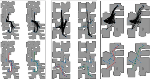
Figure 8 shows example graphs extracted from three different environments extracted with the method described in section 3.3 of the main paper.
Fig. 8: Examples of top down maps and graphs from three environments. For each environment - Top-left: topological map with ground truth connectivities, top-right: topological map with connection probabilities estimated by the learned
flink function with line opacity corresponding to the link probability,
bottom-left: ground truth shortest path between a source an target node, bottom-right: shortest path estimated by the Graph Neural Planner. Note the very bottom-right prediction connects two nodes that are not connected in the ground truth, this example would not be counted as a valid path during evaluation of the SPL metric.
7.2 Examples of Graph planner trajectories
Figures 9 and 10 of this document show additional rollouts of the hierarchical planner, complementary to figure 6 of the main paper.
7.3 Effect of the length m of the local policy
In figure 11 of this document we show the effect of the parameter m of the local policy, described in section 3, page 6, of the main document, when evaluated on a limited random subset of the validation data (1,200 problem instances).
Time-step 0 Time-step 8 Time-step 16
Time-step 48 Time-step 32
Time-step 24
Fig. 9: Six time-steps from a rollout of the hierarchical planner (graph+local) in an unseen testing environment. For each time-step: left – RGB-D observation, right
– map of the environment (unseen) withgraph nodes, source node,target node,
agent position(black),nearest neighbourto the agent, local point-goalprovided
by the high level planner andplanned path.
Time-step 9 Time-step 42 Time-step 81
Time-step 113 Time-step 170 Time-step 209
Fig. 10: Failure case - Six time-steps from a rollout of the hierarchical planner (graph+local) in an unseen testing environment. For each time-step: left –
RGB-D observation, right – map of the environment (unseen) with graph nodes,
source node,target node, agent position(black),nearest neighbourto the agent,
5 10 15 20 0.2 0.4 0.6 0.8 1.0 Success rate Paths of length 2 5 10 15 20 # inner steps 0.0 0.2 0.4 0.6 0.8 1.0 SPL Dijkstra: threshold Dijkstra: custom cost Neural Planner: deterministic Neural Planner: sampling Optimal (GT) 5 10 15 20 0.2 0.4 0.6 0.8 1.0 Paths of length 3 5 10 15 20 # inner steps 0.0 0.2 0.4 0.6 0.8 1.0 5 10 15 20 0.2 0.4 0.6 0.8 1.0 Paths of length 4 5 10 15 20 # inner steps 0.0 0.2 0.4 0.6 0.8 1.0 5 10 15 20 0.2 0.4 0.6 0.8 1.0 Paths of length 5 5 10 15 20 # inner steps 0.0 0.2 0.4 0.6 0.8 1.0 n
Fig. 11: Performance of the hierarchical agent with varied low level inner loop steps for a range of high-level path lengths.
The m parameter limits the maximum number of steps the local policy can take before giving control back to the high-level graph planner. We recall that the local policy can also decide to terminate the inner loop earlier through an explicit STOP action. We see that performance of the planner and policy is comparable up to 20 time-steps, which means the computationally costly planning step can performed less frequently than the low level control of the local policy, without a reduction in performance.
7.4 Hyper-parameters
Table 3 provides the hyper-parameters for the three different neural models used in this work:
– the explorative policy used to create the graphs, trained through RL; – the graph based high-level planner, trained in a supervised way, and – the local policy, trained through RL.
Table 3: Hyper-parameters for the exploratory policy, node linkage function and Neural Planner
Exploratory policy and Flink
Simulator resolution 64×64
optimizer Adam: betas=(0.9, 0.999), eps=1e-5
learning rate 2.50e-04
weight decay 0.0
parallel agents 16
GRU hidden size 512
Entropy coef 0.001
Advantage normalization True
Generalized Advantage Estimation True
Minibatch size 4 (trajectories)
PPO CLIP 0.1
num environment steps 200 M
TBPTT 128
Neural Planner
optimizer Adam: betas=(0.9, 0.999), eps=1e-8
learning rate 0.001 weight decay 0.0001 batch size 32 num epochs 500 dataset size 36,000 GRU size 256 Feature size 512
Learning rate decay: 0.1 every 120 epochs
GNN steps 6
Multilayer GRU Depth 2
Gradient norm clipping 2.0
Local policy
Simulator resolution 64×64
optimizer Adam: betas=(0.9, 0.999), eps=1e-8
learning rate 2.50e-04
weight decay 0.0
parallel agents 16
GRU hidden size 512
Entropy coef 0.001
Advantage normalization True
Generalized Advantage Estimation True
Minibatch size 4 (trajectories)
PPO CLIP 0.1
num environment steps 200 M