HAL Id: hal-01211774
https://hal.archives-ouvertes.fr/hal-01211774
Submitted on 5 Oct 2015
HAL is a multi-disciplinary open access
archive for the deposit and dissemination of
sci-entific research documents, whether they are
pub-lished or not. The documents may come from
teaching and research institutions in France or
abroad, or from public or private research centers.
L’archive ouverte pluridisciplinaire HAL, est
destinée au dépôt et à la diffusion de documents
scientifiques de niveau recherche, publiés ou non,
émanant des établissements d’enseignement et de
recherche français ou étrangers, des laboratoires
publics ou privés.
Data Stream Clustering for Online Anomaly Detection
in Cloud Applications
Carla Sauvanaud, Guthemberg Silvestre, Mohamed Kaâniche, Karama
Kanoun
To cite this version:
Carla Sauvanaud, Guthemberg Silvestre, Mohamed Kaâniche, Karama Kanoun. Data Stream
Clus-tering for Online Anomaly Detection in Cloud Applications. 11th European Dependable Computing
Conference (EDCC 2015), Sep 2015, Paris, France. �hal-01211774�
Data Stream Clustering for Online Anomaly
Detection in Cloud Applications
Carla Sauvanaud
∗†‡, Guthemberg Silvestre
∗, Mohamed Kaˆaniche
∗, Karama Kanoun
∗∗LAAS - CNRS, 7 avenue du colonel Roche, 31400 Toulouse, France †INSA Toulouse - 135 avenue de Rangueil, 31400 Toulouse, France
‡Universit´e Toulouse III - Paul Sabatier, 118 route de Narbonne, 31400 Toulouse, France Emails: [email protected]
Abstract—This paper introduces a new approach for the online detection of performance anomalies in cloud virtual machines (VMs). It is designed for cloud infrastructure providers to detect during runtime unknown anomalies that may still be observed in complex modern systems hosted on VMs. The approach is drawn on data stream clustering of per-VM monitoring data and detects at a fine granularity where anomalies occur. It is design to be independent of the types of applications deployed over VMs. Moreover it deals with relentless changes in systems normal behaviors during runtime. The parallel analyses of each VM makes this approach scalable to a large number of VMs composing an application. The approach consists of two online steps: 1) the incremental update of sets of clusters by means of data stream clustering, and 2) the computation of two attributes characterizing the global clusters evolution. We validate our approach over a VMware vSphere testbed. It hosts a typical cloud application, MongoDB, that we study in normal behavior contexts and in presence of anomalies.
Keywords—Anomaly detection, Data stream clustering, Cloud computing, service, MongoDB.
I. INTRODUCTION
Cloud computing is a convenient paradigm emerged for the delivery of on-demand, automated and self-managed IT resources. Infrastructure-as-a-Service (IaaS) is an example of the clouds marketing class delivering support infrastructures. IaaS allows users to deploy applications while being exempted from setting and keeping up to date the infrastructure. Virtual machines (VMs) constitute logical supports supplied by IaaS providers for the deployment of users’ applications (we call them system), with regard to the taxonomy in [6]), and distributed applications may be deployed over several VMs.
The administration of systems deployed according to the IaaS paradigm is all the more complex for IaaS providers that their VMs host a broad diversity of systems (i.e., database, management software...) with different behavioral patterns, different configurations, and workloads. Additionally, they usually do not have enough insight into all types of abnormal behaviors, referred to as anomalies, that may arise in modern systems and a large panel of them still remains due to systems complexity [10]. Anomalies may be caused by different types of faults, such as human-made faults [6] (they can be non-malicious such as misconfigurations, or non-malicious when delib-erately introduced to harm a system runtime such as denial-of-service attacks), or physical faults [6] due to the aging of hardware components for instance. Besides, anomalies may arise from both the infrastructure level and the hosted systems
level. They may propagate from one level to another and may degenerate into system failures affecting the performance of both levels. Indeed, we consider that anomalies correspond to early behaviors potentially leading to a system failure.
As a consequence, anomalies may lead to financial penal-ties for IaaS providers if service level agreements (SLAs) with users (notably related to availability and performance requirements) are not satisfied [14]. Thus, the early detection of anomalies is critical for IaaS providers.
Machine learning techniques are commonly used to sup-port anomaly detection [10]. Considering the case of cloud infrastructures with hundreds of users, VMs behaviors in normal workload contexts or in presence of anomalies are too numerous to reasonably be summarized into a labeled data set (i.e, systems observations sample labeled as anomalous or not) from which anomalous behaviors could be learned. Even though methods already exist to reduce the size of large scale problems training datasets [31], it is still intricate to forge a training dataset independently of the system type, configuration, and workload, including labeled samples of all types of anomalies [13]. To be efficient in cloud environments, anomaly detection techniques should also be designed to adapt online to frequent changes in systems behaviors that are common in such environments. (i.e., they should not raise false alarm in cases of legitimate changes in systems.
Moreover, when anomalies are detected, it is important for IaaS providers to be able to perform root cause analysis and identify potential corrective actions [1]. As a consequence, anomalies should be detected at a fine granularity, close to the components where they occur. Accordingly, the system should not be considered as a single box entity like in [11]. Such an approach leads to high-dimensional modeling problems that are tackle with difficulty [28], and it cannot specifically identify anomalous nodes in the system.
To address these issues, we present an approach to be used by IaaS providers for the online detection of unknown performance anomalies in VMs. This approach notably deals with relentless changes in systems normal behaviors during runtime. It relies on the collection of VMs monitoring data and stands on a per-VM analysis of these data. In other words, the collected VMs data are decomposed into several data streams, one stream for each VM. Each VM data stream is then structured into sub streams whose dimensions respectively correspond to counters related to the monitoring of a VM component (ex: CPU, disk, memory...). A system alarm is
raised when a least one of its VMs has a component detected as anomalous.
The numerous systems contexts to be considered led us to process monitoring data streams using clustering, a data-driven approach. Such an approach is well suited to adapt to changes in data. Our starting assumption is that anomalous behavior data are not similar to normal behavior data [10]. Moreover, we assume that normal behavior data are assigned to clusters located in a close neighborhood, and that anomalous behavior data will not be assigned to clusters located in this neighborhood.
Our approach more precisely relies on the use of data stream clustering algorithms [2], since it is the special branch of clustering coping with the online management of data streams. It executes a data stream clustering algorithm on each sub stream separately. In this study we do not propose a new version of such an algorithm and select previous methods that can fit few requirements implementations. The data stream clustering algorithm is used jointly with a new means of online characterization of the resulting clusters. It is based on the evaluation of two attributes to deal with clusters global evolution (i.e., their creation, and global movement). The clusters evolution study was introduced in the data stream clustering algorithm CluStream [3]. We perform global evo-lution characterization because we consider that individual clusters might be too numerous and evolving too fast to handle them individually like in [29]. As far as we are aware of, our approach combining data stream clustering and the characterization attributes presented in this paper is original and has not been explored in previous published work (see discussion of related work in Section VII).
We validate a simple implementation of our approach considering a MongoDB1 application deployed on a VMware based experimental testbed, using injection of anomalies by software means within VMs. MongoDB is an example of distributed database application and it is actually the most popular document store nowadays2. The experimental results demonstrate that our approach is well suited to detect anoma-lies. It performs good precision, recall (we can achieve between 99 and 94% precision, and between 99 and 85% recall), and detection latency (≤ 1min), thus confirming the above assumption about clusters.
The paper is organized as follows. Our data stream cluster-ing approach to anomaly detection is described in Section II. Section III introduces the design of an implementation of this approach. In Section IV, we present the cloud prototype on which we carried out our experiments. Section V describes our validation process. We present experimental results and discuss them in Section VI. Finally, Section VII presents the related work, and we conclude our study in Section VIII.
II. ANOMALY DETECTION APPROACH
We hereby present our approach for the case study of a single VM system. The generalization to a multi-VM system is describe in Section III.
1http://www.mongodb.org/ 2http://db-engines.com/en/ranking
The inputs of our approach are monitoring data. In more details, monitoring provides units of information about a system that are called performance counters (referred to as counters). The actual counters values being collected from a system are called performance metrics (referred to as metrics). A vector of metrics collected at a certain timestep corresponds to a monitoring observation (also referred to as observation) and an unbounded sequence of observations is called a data stream.
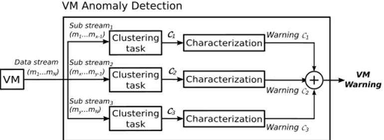
The approach is generic in that it does not depend on the specifications of the system encompassing the VM being monitored. It consists of two online steps to be reiterated upon the reception of any new VM observation: 1) the incremental update of sets of clusters by means of data stream clustering, and 2) the computations of two attributes for the characteri-zation of the clusters evolution. Both steps are represented in Figure 1 inside the Anomaly Detection entity (or AD entity). In subsection II-A, we first present implementation require-ments for the data stream clustering algorithm to be used. Indeed, our approach does not impose to use a particular algorithm but the one to be chosen should observe these requirements. Then in subsection II-B, we briefly define the sub stream partitioning for incremental update of clusters per-formed by the selected algorithm. We describe the computation of the two characterization attributes in subsection II-C, and finally present the threshold analysis based on the attributes values in subsection II-D.
VM Anomaly Detection VM Clustering task Characterization (my...mN) (mx...my-1) (m1...mx-1) (m1...mN) C1 C2 C3 Sub stream1 Sub stream2 Sub stream3 Warning C1 Warning C2 Warning C3 Data stream Clustering task Clustering task Characterization Characterization + VM Warning
Fig. 1. Anomaly detection for 1 VM, N-metrics stream, and 3 categories.
A. Implementation requirements
There is a variety of data stream clustering algorithms [2]. Our approach requires to select an algorithm that should conform to our cloud problem statement expressed in the following requirements:
a) The algorithm should not store observations neither in disk nor in RAM, since storing data steams that already have been analyzed online by our approach would not be relevant. b) The number of data clusters is not fixed a priori to keep the approach independent of systems specifications.
c) To discern clusters that have been recently updated from older and obsolete clusters, a fading cluster structure like in [4] should be used. This structure is provided by means of fading weightsapplied to observations (an example is given in the last paragraph). It is a means to make old observations die out from the clusters structures.
d) An observation counts is associated to each cluster. This count is incremented by one when the cluster is being
assigned with a new observation. Cluster fading is represented by applying fading weights on the clusters observation counts (in this case we call them weighted observations counts) like in [17].
For a set of clusters, clusters weighted observations counts are updated upon the reception of a new observation before any other data processing. Let us denote cntt,i, the weighted observation count of the ith cluster for the timestep t. With respect to this notation, the weighted observation count of each cluster is updated as the following:
cntt+1,i = 2−λ∗ cntt,i+ γt+1, (1) with λ the decay rate, γt+1= 1 if the new observation at t+1 is assigned to the ith cluster, and 0 otherwise.
B. Incremental update by means of data stream clustering Considering the study of one VM, we divide its data stream into multiple sub streams of lower dimensions. Lower-dimensional subspaces are defined according to the specific components, physical or software, their counters characterize (ex: CPU, memory, disk,...). We call the different subspaces categories of counters (referred to as categories).
Then, data stream clustering is performed on each sub stream whose dimensions correspond to one category, as presented in Figure 1. We call the incremental update of a sub stream clusters, a data stream clustering task (often abbreviated clustering task). Eventually, we obtain as many sets of clusters as there are counters categories. Figure 1 more precisely represents the clustering task of each sub stream categoryand the corresponding sets of clusters that are named CX, where X is the name of a category.
C. Characterization of clusters sets evolution
In the following we take the case of a set of clusters, CX, resulting from a single sub stream clustering task.
1) Characterization attributes: We characterize the evolu-tion of clusters in CX and thereby, their movement, by means of the study of the center of mass (CoM) of the clusters cen-ters from which we compute two numerical characterization attributes (also called attributes for short).
The CoM can be interpreted as the position where all clusters of the set are located at a fixed timestep. From the CoM position, we record the distance to the closest cluster center from the CoM, called dist min, and the distance to the farthest cluster center from the CoM, called dist max. The characterization attributes are computed as follows:
DtR Attribute. The distance from the CoM to a reference point, referred to as DtR for Distance to Reference.
A reference point can for instance correspond to the null (or the origin) vector. In our study, the reference coordinates are the mean values of observations recorded in a short training phase (see Section III for further details about the phases of our approach implementation).
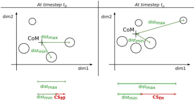
CS Attribute. The difference between dist max and dist min, referred to as CS for Cluster Spread.
The DtR and CS attributes are respectively represented in Figure 2 and Figure 3, for a two-dimension case.
DtRt0 DtRtn dim2 dim1 dim1 dim2 CoM CoM Reference Reference At timestep t0 At timestep tn
Fig. 2. The Distance to Reference (DtR) attribute for a 2-dimension case.
dim2 At timestep t0 At timestep tn dim1 dim1 dim2 CSt0 distmax distmin distmax distmax distmin distmin CStn distmax distmin CoM CoM
Fig. 3. The Cluster Spread (CS) attribute for a 2-dimension case. 2) Evolution of clusters: From this point forward we ex-plain how the attributes are used in the context of our approach. Upon the arrival of a new observation from the sub stream, the set of clusters is first updated, then the CoM, and finally the attributes are computed. For a fixed timestep (i.e., a time of update), the CoM is computed according to the following equation: CoM (CX) = 1 S n X i=1 cnti∗ vi, (2) S = n X i=1 cnti,
where n is the number of clusters in CX, vithe coordinates of the ithcluster, and cnt
i the weighted observation count of the ith cluster (introduced in Equation 1).
Some clusters might encompass observations of anomalous behaviors. Such clusters are called outlier clusters when they are detected as anomalous by our approach. This notion of outlier clusters enables us to cope with the conundrum men-tioned in [26] for data stream clustering: how to distinguish the seed of a new cluster from an outlier observation. In our study, we put all observations in clusters and then attributes characterize them either as legitimate or outlier clusters. The outlier clusters are included in the CoM computation.
3) Interpretation: Based on our experiments, both at-tributes values have a very small standard deviation over time, while recording a workload that does not change abruptly (roughly in less than 5min) and observing no anomaly in the system. Thus, the analysis of the attributes variations enables
us to monitor clusters evolution in that we consider that an abrupt change in attributes values is as an anomaly.
The variations of the CoM position from a reference point, which are represented by the DtR attribute, indicates the differences in the clusters global position over time. As clusters are not studied individually, we do not get insight into the individual movement of clusters, but into the global evolution of clusters.
Assuming that clusters representing normal behaviors are located in a close neighborhood, individual creations, deletions or shifts of legitimate clusters do not dislocate the CoM enough to be detected as anomalous events.
The changes in the DtR attribute mean value indicate modifications in behavior trends. Such modifications can result from workload changes, anomalies or VM reconfigurations. For instance, given the upgrade of a VM memory from 1Gb to 10Gb, clusters computed before the reconfiguration will be different from clusters computed after the reconfiguration since metrics change in scales. The corresponding CoMs will accordingly differ and be at different distances from the reference point. The changes in the CS attribute mean value are likely to be provoked, when they are abrupt, by the creation of a new cluster that is not in the close neighborhood of other clusters, as it is way farther from the CoM than the last farther cluster already was. This corresponds to the creation of an outlier cluster. We consider that anomalies arise more abruptly in a system than workload changes. The distinction made by the attributes between workload changes and anomalies is further discussed in view of results in Section VI.
4) Outlier detection and possible evolution: Outlier clus-ters are identified as such by both the DtR and the CS attributes as abrupt changes in their mean value. The growth of the observation count of an outlier cluster and the creation of several clusters near this outlier cluster may be observed. In this case, the CoM moves toward the new group of clusters, and thereby alters the DtR value, and the CS attribute de-creases. The CoM may finally stabilize with both attributes. Old clusters are discarded from the set by their weighted observation count, and the clusters that were once outliers are regarded as representative of a new legitimate system behavior. In our approach, old clusters are pruned on a threshold basis. A cluster is pruned when its weighted observation count is less than a threshold we call prune threshold (denoted tprune). The speed of the CoM shift from the reference point depends on tprune and λ. The higher these parameters are, the faster the CoM leans toward new clusters and the faster the set of clusters evolves so as to represent a new behavior or a new workload. The clusters evolution consequently depends on both parameters.
5) Handling workload variation: A large tprune and a large λ lead to fast discarding of clusters. In this case, new observations may often be assigned to newly created clusters, whereas they could have been assigned to recently discarded clusters. Consequently, the CoM may vary between a fixed number of recurrent positions. The attributes values may also steadily oscillate showing the persistent creation of new clusters. It could potentially lead to the detection of False Positive (FP) if the anomaly detection based on the attributes values is parametrized with a variation threshold set too low.
Two methods are conceivable for the calibration of our approach to well handle workload variations. A first method consists of using large values for tprune and λ. It reduces the mean number of clusters in the clusters set and makes the shift of the CoM toward new clusters quicker. However, it may lead to the detection of FP since many new clusters would be repeatedly created and detected as outliers.
Another method consists of selecting really small values for both parameters so that the set of clusters contains a large number of clusters representing all types of past behaviors or workloads. It is relevant considering that the workloads vari-ations may bring the system into previously seen workloads, however numerous they might be. Yet, it leads to the increase of the number of clusters and induces higher computation costs. As a result, in our validation process we use tprune and λ that correspond to a trade off between both methods (see Section VI).
D. From attributes to warnings
A VM warning is raised when an anomaly is detected in at least one of its sub streams. Anomalies are detected when attributes values exceed a given threshold for a fixed number of consecutive timesteps. We call this number of consecutive timesteps warning count (denoted W). Considering one at-tribute a and for a given timestep t, the threshold corresponds to the following equation:
T hreshold(a, t) = mean(a, t) ± (N ∗ sd(a, t)), (3) where N is a positive integer called warning coefficient, mean(a, t) and sd(a, t) are respectively the moving mean and the moving standard deviation of the attribute values at timestep t.
The same moving window size (called mw size) is consid-ered for computing mean(a, t) and sd(a, t) for both attributes. The moving mean value at t is the mean of the last mw size attribute values. Expressly, it uses a moving mean with a mw sizeoffset value, and mw size is expressed in number of values, i.e., instance of attribute update.
By definition, the moving window introduces a lag behind the true value of the local mean. The larger mw size is, the bigger is the lag. On the other hand, a small mw size enables us not to get a moving mean too much shifted in time and so, detect anomalies shortly after they occur. Also, a small mw size does not require to undervalue the old datum composing the sample window so as to simulate data aging (see [18] for examples like weighted moving mean). As a consequence, in our study we will consider small mw size.
We highlight that the clusters relate to the history of the system (that can be as old as few hours of few days) that is still relevant at the present time. Our approach has the advantage to combine the memory of old behaviors of the system and the runtime awareness needed for fast anomaly detection. In comparison, an approach that would only use of a moving window analysis applied to raw observations would lose relevant insight into the system history as soon as old observations are not part of the window.
III. IMPLEMENTATION
This section presents an implementation of the aforemen-tioned approach, generalized to the case of a multi-VM system. It is drawn on a two-phases that we present in subsection III-A. Subsection III-B describes the overall implementation. A. Two-phase operation
Our implementation is based on two distinct phases: a training phase followed by a detection phase.
The training phase takes place while the system runs a workload that represents one probable use of the system and reasonably assuming that no fault is activated. During this phase, we record from all the system VMs a fixed number of observations that can be as low as few hundreds. Observations of each VM are partitioned according to counter categories so as to compute reference points for each category of each VM: the points coordinates are the respective mean values of the per-category observations. These points can be later used for the DtR attribute computation during the detection phase. This phase also enables us to get an estimation of the mean and standard deviation of the observation metrics. They are used for the pre-processing of observations before clustering tasks. Indeed, it can be valuable for some clustering algorithms to normalize or even standardize observations (i.e., removing the mean value and dividing by the standard deviation) before assigning them to a cluster. It is due to some clustering algorithm using a fixed threshold to assigned observations to clusters, with no regard to the data distribution. The training phase is to be run once, as the system is being deployed. It may potentially be run after the system undergoes large reconfigurations or after major anomalies have been located and removed. Lastly, this phase is short and takes less than 1sec to be executed.
The detection phase performs the anomaly detection during the rest of the system runtime. It requires the mean and standard deviation values resulting from the training phase so as to standardizing the system data streams.
B. Overall functioning
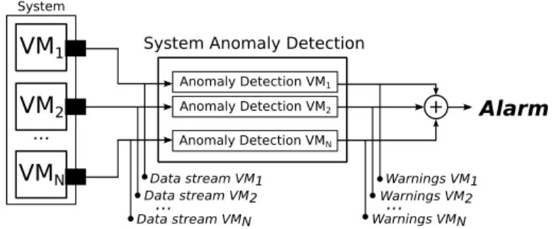
Considering a multi-VMs system, anomaly detection is performed on a per-VM basis, with each VMs data stream being independently analyzed. The overall functioning for a N-VMs system is represented in Figure 4.
System
System Anomaly Detection
Warnings VM2 Warnings VMN
VM
1VM
2VM
N Alarm Warnings VM1 Data stream VM1 Data stream VM2 Data stream VMN... ... ... Anomaly Detection VM1 + Anomaly Detection VMN Anomaly Detection VM2Fig. 4. Anomaly detection implementation for a N-VMs system.
Observations are collected by monitoring agents (repre-sented as black boxes in Figure 4) and are then fed to
the system AD entity. This entity implements the anomaly detection approach presented in Figure 1. One instance of VM AD entity is run in parallel for each VM of the system. System alarms are raised when at least one VM AD entity detects an anomaly and therefore, raises a warning. When they receive an alarm, administrators work on the root cause analysis keeping in mind that they are provided with the specific anomalous VMs and components. Alarms should be transmitted to the user in case administrators assume they are only correlated to the user’s system. The end of a warning may signify that either the effects of the anomaly are dissipated or the system remains in a anomalous state, and the AD entities got used to it. We note that it should be apparent to the administrator that an anomaly actually persists in the system, since we assumed that the persistence of anomalies lead to failures and SLAs violations.
IV. EXPERIMENTAL SETUP
This section describes the testbed on which we set up our experiments for the case study of a MongoDB system.
A. Infrastructure description
We conducted our experiments on a VMware vSphere 5.1 private platform. The infrastructure is composed of two servers Dell Inc. PowerEdge R620 with Intel Xeon CPU E5-2660 2.20GHz and 64GB memory. Each server has a VMFS storage and they also share a NFS storage. One hypervisor hosts all VMs related to the MongoDB system (referred to as system host), the other hypervisor is a controller that hosts the monitor as well as the workload generator for isolation concerns.
B. Case study description
Our case study is MongoDB release 2.4.8. It uses 2 partitions of 3 data replicas (i.e., 6 VMs). Each VM has a 14GB disk, 4 virtual processors, 1Gbps network interface, and 4GB of RAM. The MongoDB behavior is assessed while running the Yahoo! Cloud Serving Benchmark [12] workload.
C. Monitoring setup
For the sake of our study, we implement a monitoring entity centralizing all VMs data streams in a database. It enables us to store monitoring observations in different datasets collected from different experiments for later analyses.
We used the Ganglia monitoring system [21] to collect metrics from our MongoDB system. Ganglia is a general purpose monitoring tool for distributed systems. We deployed one monitoring agent on each VM. No specific counter related to MongoDB is being collected by the agents since we want to validate our approach with no dependency with the user’s application type. We study 89 counters that are split according to five categories: CPU, memory, disk, TCP, and IP. Further information about the collected counters is available online3. Metrics are collected every 15sec from each VM.
D. Data stream clustering implementation
In our study, we use the GNU R implementation of the data stream clustering approach from [17]. It is a simple implementation of the threshold nearest neighbor algorithm. It is easy to handle and complies with our assumption that observations in case of normal behavior are located in a close neighborhood [10]. Also, this implementation does not store data in disk or RAM, and does not work with a prior assumption about the number of clusters to be found in data. The clustering algorithm makes use of the general weighted observations counts handling method presented in Equation 1. Considering a set of clusters, upon reception of a new observation, weighted observations counts are updated, and clusters being too old are pruned. At any time, the model is described by the current clusters centers (in this study we use centroids), as well as their respective weighted observation count. Then, the distance between the observation and all clusters centers is computed. The observation is assigned to the closest cluster with a distance smaller than a given threshold we call neighbor threshold or tneighbor. When no cluster is close enough, a new cluster is created. As a consequence, the neighbor threshold tempers the local variations of the observation metrics.
We selected the Euclidean distance for our computations because it is the most commonly used measure [10] and it is fast to compute. The observations standardization processed over system data streams enables us to cope with the great sensitivity of the Euclidean distance toward the metrics scales.
V. VALIDATION METHOD
Our validation method is twofold. In a first phase we test the ability of our detection approach to well handle normal behavior case scenarios. In such scenarios, our approach should not identify any anomalous behavior, and therefore, not raise any alarm. We test this ability by means of the FP ratio quantifying the proportion of false alarms raised while working on observations of normal behavior workloads.
The second phase consists in testing our approach over scenarios comprising both normal and abnormal behaviors. In such scenarios, we validate the ability of our approach to raise an alarm when detecting an abnormal behavior, i.e., an anomaly. Such scenarios are built from the superposition of a faultload to a normal behavior workload. Faultloads are scenarios of anomaly injections emulating the effect of faults activations. We test this ability by means of three measures, namely precision, recall and detection latency. These measures qualify the detection power of our anomaly detection approach. We define the detection latency as the number of updates (i.e., observation reception) between the injection of an anomaly and the corresponding alarm being raised thanks to at least one sub stream attribute.
We record several datasets from our experimental setup, and store them in a database so as to enable backward analyses. There is a broad spectrum of real case workloads and faultloads and we present the study of six such cases, that we find to be general cases. Observations from these datasets are fed to the implementation of our approach incrementally.
A. Normal behavior validation
We record datasets of normal behavior observations from the 6 VMs of our MongoDB system, while running the system under four different normal behavior workloads.Datasets (1–4) are recorded while respectively running each workload.
Workload (1). Running an average rate of 3000 read operations per second. Without any other administration task being run on the system host. The dataset encompasses 69,120 observations (i.e., over two working days monitoring).
Workload (2). Running an average rate of 3000 read operations per second. With additional administration tasks being run on the system host: a network dump over 20min, a VM memory reconfiguration allocating a test VM with one more GB of memory, a VM memory reconfiguration so as to allocate all the host free memory to a test VM, and a VM migration from the system host to the controller host. Each task is separated by 1h from the last task before it. The test VM is running on the system host and is not part of the MongoDB system. The dataset encompasses 34,200 observations.
Workload (3). Running an increasing ramp of read opera-tions rates, from 1000 to 4000 operaopera-tions per second and each load lasts 1h. The pattern is repeated 10 times. Without any other administration task being run on the system host. The dataset encompasses 57,600 observations.
Workload (4). Running read operations with different rates, 10min each rate, using the following pattern: (1000, 2000, 3000, 2000, 1000, 3000, 1000, 2000) operations per second, and the pattern being repeated 10 times. Without any other administration task being run on the system host. The dataset encompasses 19,686 observations.
B. Validation in presence of anomaly
Faultloads encompass injections of widespread anomalies existing in real scenarios of our field. Such anomalies are supposed to arise from software and hardware faults. We emulate them by software means. Five types of anomalies are included in our faultload, namely 1) CPU consumption, 2) misuse of memory, 3) anomalous number of disk access, 4) packet loss, and 5) network latency (respectively referred to as CPU, memory, disk, packet loss, and latency anomalies). In the following, we present examples of real scenarios leading to these anomalies, then we describe the different intensity levels at which the anomalies may be injected into a system and finally present the implementation of the faultloads.
1) Types of anomalies: We selected anomalies so as to emulate the following behaviors.
CPU consumption. Anomalous CPU consumptions may arise from faulty programs encountering impossible termina-tion conditermina-tions leading to infinite loops, busy waits or dead-locks of competing actions, which are commonplace issues in multiprocessing and distributed systems.
Memory leaks. Anomalous memory usages are common-place in programs whose allocated chunks of memory are not freed after their use. Accumulations of unfreed memory may lead to memory shortage and system failures.
Anomalous number of disk access. A high number of disk accesses, or an increase in the number of disk accesses
over a short period of time, emulates anomalous disks whose accesses often fail and lead to an increase in disk access retries. It may also result from a faulty program in infinite loop of data writing.
Network anomaly. Network anomalies may arise from network interfaces or the interconnection of networks. In this work we emulate packet losses, and latency decreases. Packet losses may arise from undersized buffers, wrong routing policies and even firewall misconfigurations. As for latency anomalies, they may originate from queuing or processing delays of packets on gateways.
2) Intensity levels: Each anomaly has a range of intensity levels that we calibrate thanks to prior experimentations (see our previous work [27]). Regarding the memory, disk and CPU anomalies, the maximum intensity value of an anomaly is constrained by the capacity of VMs operating systems. Considering the remaining types, the maximum intensity value is set so as not to lead to a VM failure but to be close to. Intensity levels are described in Table I.
TABLE I. ANOMALY TYPES AND INTENSITIES.
Type Unit Intensity levels
1 2 3 4 5 6 7
CPU consumption % 30 40 50 60 70 80 90
Misuse of memory % 79 82 85 88 91 94 97
Disk access #workers 20 25 30 35 40 45 50 Packet loss % 3.2 4.0 4.8 5.6 6.4 7.2 8.0
Network latency ms. 32 40 48 56 64 72 80
3) Implementation: Faultloads are run at the VM level. Injections are performed by three programs run on each VM. They are triggered by means of ssh connexions orchestrated by a campaign handler. The campaign handler is a configurable script hosted on the controller host.
We use Dummynet4 for the injection of network latency and packet loss anomalies, and Stress-ng5 for CPU, disk, and memory anomalies.
4) Faultloads and datasets: Datasets (4) and (5) are recorded while running Workload (1), respectively running the following two faultloads. We make use of Workload (1) as a common workload.
Faultload (1). All types of anomalies are being injected. Anomalies of the same type were injected consecutively in each VM and in increasing order of intensity values. Each injection of a given intensity was injected 6 times, one time consecutively in each VM. The injections last 10min. Two consecutive injections were 20min apart, and triggered in a different VM. Thus, two consecutive injections in one VM are 2h50 apart. The dataset encompasses 336,000 observations.
Faultload (2). All types of anomalies are being injected with their respective intensity level 5 but with injections spaced by 10h. Therefore, it notably differs from Faultload (1) in that it has a different duration separating two consecutive injec-tions. We consider that both Faultload (1) and (2) represent worst case studies since anomalies are very close, and no
4http://info.iet.unipi.it/∼luigi/dummynet/ 5http://kernel.ubuntu.com/∼cking/stress-ng/
VM is restarted. Therefore, anomalies might accumulate in the system. The dataset encompasses 380,000 observations.
For both faultloads, the duration of anomalies was set to 10min. Moreover, as we will expose later, in worst cases, in worst case scenarios, our approach can take until 4min to detect an injection after it is triggered, so we do not consider injection durations less than 4min.
VI. RESULTS ANDDISCUSSIONS
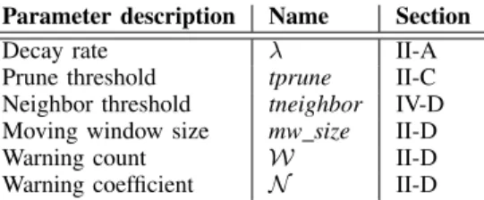
We hereby present the results, in terms of FP ratio and detection power, of the different validations we run over our 6 datasets. For successful validation, we perform parameter tuning of the six parameters on which our approach depends. We remind them in the following table, with the section they were first introduced in this paper:
Parameter description Name Section Decay rate λ II-A Prune threshold tprune II-C Neighbor threshold tneighbor IV-D Moving window size mw size II-D Warning count W II-D Warning coefficient N II-D
We distinguish two sets of parameters. λ, tprune, and tneighbor are related to the implementation of the data stream clustering algorithm used in the clustering tasks of our ap-proach (see II-B). mw size, W, and N are related to the characterization of the clusters sets by our attributes (see II-C). Parameter tuning is performed so as to obtain ranges of parameters values that enhance the detection power and reduce the FP rates of our implementation. In the following, we first present the tuning of the first set of parameters in subsection VI-A. This allows us to set a value for these parameters, given that they reasonably lead to low FP rates and good detection power. We then tune the second set of parameters in subsection VI-B, with respect to the fixed values selected for the first set. Finally we present three discussions in subsection VI-C about the time between anomalies to be used in faultloads, the discernment between anomalies and workload changes, and about the necessary use of both attributes.
Due to space limitations, we only present the most signif-icant results and summarize the rest of them.
A. Tuning of parameters related to the clustering algorithm We discuss the tuning upon λ, tprune and tneighbor with respect to the study of Datasets (1), (2), (3), (4), and (5) (wwith (5) encompassing a faultload). We first consider for each parameter a range from 0.1 to 0.5 by 0.1, and then, another range with smaller pace, from 0.001 to 0.01 by 0.001. These three parameters impact the mean number of clusters in the set of clusters of a sub stream. The mean value of the number of clusters depends on the sub stream category. Some sub stream categories appear to be more sensitive to the thresholds changes (i.e, tprune and tneighbor) than others. It is explained by both the number of dimensions of the sub stream categories and the metrics variations. In other words, sub streams with high dimensions and each metric varying a lot, tend to lead to a large number of clusters.
Considering the discussion in II-C about the impact of varying tprune and λ, we select trade off values for these pa-rameters in order to maximize the number of clusters being in a set and minimize the computation costs. We experimentally selected parameters λ = 0.1, tprune = 0.1, and tneighbor = 0.001 because they jointly provide good timing performance for the clustering tasks and characterizations, a low FP rate for Datasets (1), (2), and, (3), and a good detection power for Dataset (5). These values are however not adapted to Workload (4) which encompasses too abrupt and quick variations of the number of queries per second. The reader should note that in real case studies, there would be some smoothing in the variation of the number of queries compared to Workload (4), so our approach would perform better for real workloads. Corresponding results for these datasets are presented in the next subsections which present the tuning of the rest of the parameters. They lead to sets of clusters with an average between 5 and 11 ± 3 clusters, depending on the sub stream category. The update of a set of clusters making use of an average of 11 ± 3 clusters with 11 dimensions, and after the corresponding characterization task, is performed in 0.021s. Note that we applied the same tneighbor values for each sub stream category for simplicity concerns.
B. Tuning of parameters related to the characterization at-tributes
We now present the results of the tuning of the second set of parameters with the first set being (λ, tprune, tneighbor) = (0.1, 0.1, 0.001). We start with the study of normal behavior scenarios only and tune parameters so as to minimize the FP rate of our approach. Then, we study the alarms raised in presence of faultloads, and tune parameters so as to maximize the detection power (increase precision and recall, and decrease detection latency).
1) Study of normal behavior datasets: We first perform a coarse grain tuning of the window size over the four datasets of normal behavior workloads. We find that considering a window size over 40, the attributes means are too much shifted from the actual value (in other words, the lag is too important), and the FP rate starts increasing over 10%. Therefore we set the tuning range of mw size in [8; 40].
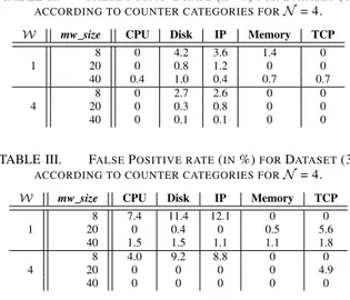
Then, we consider the tuning of W for Datasets (1), (2), and (3). As expected, results show that the FP rate is inversely proportional to W. However, the larger W is, the worst our detection power is expected to be during the study of datasets with faultloads. Indeed, the detection latency is systematically reduced by the waiting of W updates to raise an alarm (see next subsection VI-B2). Accordingly, we experimentally find a range of W values that encompasses the W values that can achieve a FP rate lower than 15%: [1; 4]. While varying mw size between 8 and 40 and W for both of its range endpoints, our approach successfully leads to a small FP rate between 0 and 4.2% for Dataset (1) and (2), and between 0 and 1.21% for Dataset (3). We note that the larger mw size is, the more local variations are attenuated. Consequently, it leads to lower FP rates in cases of stable attributes values. Table II and Table III, respectively present the FP rates for Datasets (1) and (3). Each column corresponds to the FP rate of one counter category. We record similar results for Dataset (2) compared to Dataset (1).
TABLE II. FALSEPOSITIVE RATE(IN%)FORDATASET(1)
ACCORDING TO COUNTER CATEGORIES FORN = 4.
W mw size CPU Disk IP Memory TCP
1 8 0 4.2 3.6 1.4 0 20 0 0.8 1.2 0 0 40 0.4 1.0 0.4 0.7 0.7 4 8 0 2.7 2.6 0 0 20 0 0.3 0.8 0 0 40 0 0.1 0.1 0 0
TABLE III. FALSEPOSITIVE RATE(IN%)FORDATASET(3)
ACCORDING TO COUNTER CATEGORIES FORN = 4.
W mw size CPU Disk IP Memory TCP
1 8 7.4 11.4 12.1 0 0 20 0 0.4 0 0.5 5.6 40 1.5 1.5 1.1 1.1 1.8 4 8 4.0 9.2 8.8 0 0 20 0 0 0 0 4.9 40 0 0 0 0 0
From this point forward, we perform the tuning of N for Datasets (1), (2), and (3), but only present results for Dataset (1) as the study of the other two datasets leads to the same conclusion. We chose the same value of N for both attributes thresholds (see Equation 3). W = 1 and mw size= 40 both minimize the FP rate, therefore we select these values while varying N . Results are presented in Table IV. They show a coherent decrease of the FP rate as the warning coefficient is being increased, since the threshold is proportional to N . The FP rates vary between 70% for N = 1, and 0 for N = 5. We record that the FP rate is acceptable from N = 3, with a mean of 3.1%. We should keep in mind that the detection threshold of attributes (see Equation 3) is proportional to N . Therefore, its increase will lead to higher False Negative rates in datasets with faultloads. Thus, we select a trade off value of N = 4.
TABLE IV. FALSEPOSITIVE RATE(IN%)FORDATASET(1)
ACCORDING TO COUNTER CATEGORIES FORmw size= 40,ANDW = 1.
N CPU Disk IP Memory TCP
1 71 71 66 61.3 60.4
2 17.7 17.5 17.3 17.8 14.8
3 2.7 3.9 2.4 3 2.5
4 0.4 1.0 0.4 0.7 0.7
5 0 0.2 0.1 0 0
Finally, Table V presents the FP rates for the individual study of Dataset (4), using the aforementioned selected values: N = 4, mw size = 40, and W = 1. We record that it leads to higher FP rates, compared to Datasets (1), (2), and (3), with an FP rate between 6.1% to 22.5%. It is linked to the fast change in the number of queries sent to our system in this dataset.
TABLE V. FALSEPOSITIVE RATE(IN%)FORDATASET(4)
ACCORDING TO COUNTER CATEGORIES FORN = 4, mw size = 40,AND
W = 1.
N CPU Disk IP Memory TCP
4 6.1 19.4 22.5 10.9 6.4
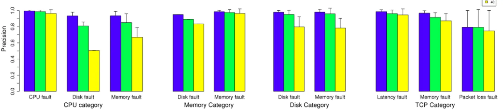
2) Study of datasets with faultload: The following presents the tuning of mw size, with N = 4, W = 1, and mw size in (8, 20, 40). Figure 5 and Figure 6 respectively present the precision and recall obtained for Dataset (5), for the detection of all types of anomalies, and for the sub stream categories which achieve both a precision and recall higher than 75% for
Fig. 5. Precision of detection for Dataset (5) with standard deviation, by sub stream categories, for mw size ∈ (8, 20, 40), with N = 4, and W = 1.
Fig. 6. Recall of detection for Dataset (5) with standard deviation, by sub stream categories, for mw size ∈ (8, 20, 40), with N = 4, and W = 1.
Fig. 7. Detection latency for Dataset (5) with standard deviation, considering a 15sec monitoring period, for mw size ∈ (8, 20, 40), with N = 4, and W = 1.
at least one value of the range of mw size. We record similar results for Dataset (6). In both datasets, the IP sub stream category do not perform good enough precision and recall and it is not represented in the figures. The corresponding detection latencies are presented in Figure 7.
We observe that our approach enables us to detect all anomalies thanks to the characterization attributes of at least one sub stream category. These anomalies are detected with fair precision and recall, i.e., between 75 and 98%. Globally, the detection power tends to be better as the mw size decreases, that is to say it is the opposite tendency of the FP rates (see subsection VI-B1). For mw size ∈ [8;20], we achieve a precision between 99 and 94%, and recall between 99 and 85%. Accordingly, we recommend to use a trade off value for mw sizewhich would be 20.
In more details, we identify that the CPU, disk, and TCP sub stream categories are sufficient to detect all anomalies
with enough precision and recall. Thus, our approach has the aptitude to perform without the knowledge of application spec-ification (here MongoDB), as it does not hinge on monitoring data directly related to it, but only on OS related counters.
Besides, we also notice that the injection of anomalies of a given type may be detected by several sub stream categories. For instance, the injections of memory anomalies are detected by all sub stream categories. This is due to the escalation of anomalies effects. In real case scenarios, memory anomalies may be linked to faulty tasks, either created by the user’s application or by the OS, that are consuming CPU resources for instance. Also, an anomaly in a program with network sockets can potentially result (by error propagation) in bad packet formations, and thus be detected by the TCP sub stream category.
With respect to the detection latency, we observe short latency (≤ 1min) for the detection of injections by the CPU,
the memory, and the disk sub stream categories, and also by the TCP category for memory anomalies, given a 15sec monitoring period. We record a detection latency between 1 and 2.3min for latency and packet loss anomalies detected by the TCP category.
Finally, we observe that the IP counter category cannot perform sufficient precision nor recall for the detection of any type of anomaly. Further analysis led us to the conclusion that the IP counter category has too high variability metrics. The same point can be noted for the TCP counter category even if it still performs good enough detection power with the provided parameters configuration. Indeed, network related metrics has high variability. Retrospectively considering the tuning of the first set of parameters, we recommend using a larger tneighbor (the tolerated threshold for the assignment of an observation to a cluster) for the specific update of the TCP and IP counter categories. Since metrics of these categories seem to be highly changing in short periods of time, a higher tneighbor for this specific sub stream category should lead to results with a variability similar to the one of other sub streams.
C. Discussions
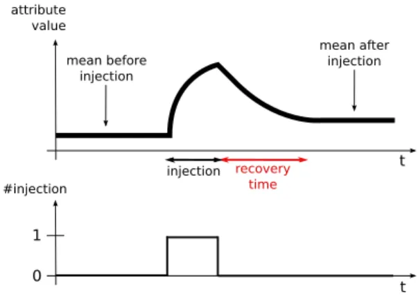
1) What recovery time between anomaly injections?: Dur-ing experimentations, we noticed that after an injection and without any external recovery action, the metrics values of the VM being injected are slowly auto-recovering from the effects of the injection. A certain recovery time is needed to dissipate the effects of anomalies injected (we remind that we run experimentation in worst case scenarios with no VM restart and anomaly injections effects might never totally dissipate). The recovery time is illustrated in Figure 8. It corresponds to the time between the end of an injection and the time at which our attributes stabilize back to a new mean value. Note that the new mean value of the attributes may not be the same as before the injection, since we do not restart the VMs after injections and errors might accumulate.
t #injection t 1 0 attribute value mean before injection mean after injection recovery time injection
Fig. 8. Recovery time for an attribute value after one injection.
We experimentally find that 110 observations (i.e., 30min with a 15sec monitoring period) corresponds to the worst number of instances needed to get either one attribute to stabilize to a new mean value after an injection. This number depends on both the type of anomaly and the attribute being considered. For example, we record that regardless of the injec-tion durainjec-tion, it takes around 10 instances for both attributes to stabilize after the injection of a CPU anomaly but around 110
instances considering a memory anomaly. As a consequence, in Dataset (5), two consecutive anomalies injected in a single VM are separated by more than 30min (around 3h apart).
Lastly, our approach raises alarms during the recovery time, and while validating our approach such alarms are considered to belong to the same anomaly.
2) How to differentiate workload changes and anomalies?: While questioning the difference between workload changes and anomalies, we observed that the characterization attributes are slower to get back to a stable value after an injection than when they are altered by variations of queries rates such as in Workloads (3) and (4). This short stabilization time while running Workloads (3) and (4) implies few deviations of the attributes values, and led us to obtain low FP rates for the corresponding datasets. This is explained by variations in query rates smoothly and slightly impacting metrics.
Anomalies, on the other hand, greatly impact metrics. Counters like memory mapping for instance, are greatly im-pacted by memory anomalies but hardly by query rates varia-tions. This particular example is due to the fact that query rates variations do not influence the mapping of the database files in memory but anomalies do. Indeed, MongoDB automatically uses all free memory of VMs regardless of the queries rates. Memory anomalies reduce the free memory space and impact the MongoDB system behavior.
3) Is one attribute enough for detection?: We tested the detection power of our approach on Datasets (1) and (5) by considering respectively the alarm output of the DtR attribute, the CS attribute, and also their joint alarm output, i.e., a warning is raised when at least one attribute raises a warning or when both attributes raise a warning. In terms of detection latency we find that no injection is detected quicker by an attribute in particular. Besides, there is no attribute that would be best suited to the detection of one particular anomaly or to the detection of anomalies in one particular counter category. The joint use of both attributes by raising a warning when either one of the attribute raises a warning provides the best results.
VII. RELATED WORK
As modern software systems always grow in complexity, it became all the more complex to get an accurate understanding of systems during runtime [19], [23]. The dynamic of a system runtime can be reflected by several means like the systems logs [20], [32], kernel and file system traces [22], or the monitoring data [13], [27]. In such a work as Dtrace [8], the authors insert probes of monitoring data and actions to be executed when probes are matched, into an application being troubleshooted. However the probes definition is fastidious and makes such rule-based efforts unsuited for data driven exploration in large scale systems. The monitoring of clouds is surveyed in [1].
In order to deal with unknown systems behaviors and potential anomalies, administrators may used reactive methods as anomaly detection. Anomaly detection aims at identifying patterns in data that do not fit an expected behavior [10]. Broadly, the identification of specific data patterns can be performed by means of supervised or unsupervised methods. Supervised methods require prior knowledge about systems
and labeled training datasets. [11], [24], [28], [32] are such examples, respectively working on detecting anomalies by means of Tree-Augmented Bayesian Networks (TAN), Princi-pal Component Analysis (PCA) associated with decision trees, Semi-Hidden Markov models, and Two-dependent Markov models used conjointly with TAN. Another example is our previous work [27], applying a Support Vector algorithm for in scale-out storage systems.
Since it is not always possible to acquire samples of anoma-lous behavior data and label them in a training dataset, such works as UBL [13] exploit unsupervised methods. With regard to our consideration that anomalies are early behaviors leading to failures, UBL well performs the detection of unknown anomalies in clouds with Self Organizing Map representing virtualized resources by means of neurons. However, normal behavior profiles are not easily updated in an online fashion. In [25], the authors introduce an algorithm for the case of un-labeled data that learns a single data boundary from a training dataset representing the normal behavior of a system (i.e., one class classification). They consider that a data item that lies outside the boundary that has been learned is anomalous. In our study, we do not rely on one class classification or methods as UBL, and propose an approach that tackless during runtime the dynamic characteristic of systems, whose normal behaviors in the future depend on unstable environments. Data stream clustering algorithms are data-driven approaches that can deal with dynamic systems, and perform clustering on data provided in an incremental manner. A survey is presented in [2].
It is worth to be mentioned that with a high-dimensional data space comes a potential sparsity of data [7], i.e., the difference between two data points is almost null. As a results, when high-dimensional data spaces are not handled properly, the relevance of anomaly detection approaches can decrease [28]. Several approaches deal with reducing data space dimensionality such as in [16] using PCA, or in [15], by means of two methods for metric selection and combinations. These works aim for the enhancement of methods analyzing large datasets such as anomaly detection. Nevertheless, they lead to new dimensions which interpretation is fastidious [5]. Some data stream clustering algorithms tackle the high dimensional datasets issues in their implementation. In [5] the authors well tackle high-dimensionality with the data stream clustering algorithm CLIQUE, by automatically locating high-density clusters in dimension subspaces. In our study, we do not use dimension reduction techniques. As in [13], [28] we divide high-dimensional systems data streams into VMs data streams, and in comparison we then again partition VMs data streams into lower-dimension sub streams whose dimensions respectively correspond to VMs components. In enables us to ease root cause analysis when anomalies are detected.
In related works, clustering algorithms are often used as a task for a first pre-processing in other mining processes or clas-sification problems [33]. In comparison, our approach proposes an online characterization of clusters based on the evaluation of two attributes to deal with clusters global evolution, and it is to be used conjointly with a simple data stream clustering algorithm. Considering works on the evolution of clusters movements, the data stream clustering algorithm CluStream [3] includes a clusters global evolution study in itself. However, it is processed in an offline component, and it needs prior
knowledge of the number of clusters to be found in data. Thus, it supposes prior knowledge about system specification. MovStream [29] is an approach for the study of clusters move-ments but performed individually. In our study, we assume that individual clusters might be too numerous and evolving too fast to handle them individually with individual significant implication. Examples of algorithms that can be used in our approach are D-Stream [30] and DenStream [9], two well known density-based data stream clustering algorithms. They do not require a parameter corresponding to a number of clusters. Also, in [17], the authors present an implementation of threshold nearest neighbor data stream clustering algorithm that also does not make use of such a parameter.
As for the validation of a large body of data stream clustering methods, they are performed on synthetic datasets and real datasets from major fields like charitable donations (KDD’98) [9], and network intrusion detection (KDD’99) [30]. In comparison, we work on datasets from a virtualized infras-tructure testbed. To our knowledge, data stream clustering has not been used by means of global characterization of clusters evolution for online anomaly detection in virtualized cloud environment in previous published work.
VIII. CONCLUSIONS ANDFUTURE WORK
In this paper we introduced a new approach for online anomaly detection based on data stream clustering and the characterization of the clusters global evolution by means of two numerical attributes. This approach notably deals with relentless changes in systems normal behaviors during runtime and detect unknown anomalies. We presented a simple imple-mentation of it considering a MongoDB application deployed on a VMware based experimental testbed, and shown its performances using injections of anomalies.
The detection is based on the processing of the monitoring data streams of the VMs composing a system. Such streams are analyzed separately, and each one is being partitioned into sub streams of lower dimensions that correspond to group of counters related to the same VM component. The parallel clustering of each VM sub streams makes our approach scalable to systems of any number of VMs. Moreover, our approach is generic in that it does not require any specification of the systems being analyzed. This generic functioning, which is a prerequisite for applications to cloud environments, makes it applicable to other anomaly detection environments.
Our implementation achieves between 75 and 98% of precision and recall for the detection of anomalies such as CPU consumption, memory leak, anomalous number of disk access, network latency and packet loss, and with detection latency less than 1min for all our anomalies except latency anomalies that are detected within a mean of 2min.
As for future work, an extensive study about other types of MongoDB workloads (write and update queries) should be carried out. We also intend to apply our approach to the study of another example of cloud application. Finally, we aim to work on an entity in charge of correlating the system VMs warnings depending on which VMs and on which sub streams anomalies originate. Indeed both VMs roles (router, data replica...) and anomalous components may be consider to raise an alarm.
ACKNOWLEDGMENTS
This work has been carried out in the context of the Secured Virtual Cloud project, a French initiative to build a secured and trustworthy framework for cloud computing.
REFERENCES
[1] G. Aceto, A. Botta, W. de Donato, and A. Pescap, “Cloud monitoring: A survey,” Computer Networks, vol. 57, no. 9, pp. 2093 – 2115, 2013. [2] C. C. Aggarwal, “A survey of stream clustering algorithms,” in Data
Clustering: Algorithms and Applications, 2013, pp. 231–258. [3] C. C. Aggarwal, J. Han, J. Wang, and P. S. Yu, “A framework
for clustering evolving data streams,” in Proceedings of the 29th International Conference on Very Large Data Bases - Volume 29, ser. VLDB ’03. VLDB Endowment, 2003, pp. 81–92.
[4] ——, “A framework for projected clustering of high dimensional data streams,” in Proceedings of the Thirtieth International Conference on Very Large Data Bases - Volume 30, ser. VLDB ’04. VLDB Endowment, 2004, pp. 852–863.
[5] R. Agrawal, J. Gehrke, D. Gunopulos, and P. Raghavan, “Automatic subspace clustering of high dimensional data for data mining applications,” SIGMOD Rec., vol. 27, no. 2, pp. 94–105, Jun. 1998. [6] A. Avizienis, J.-C. Laprie, B. Randell, and C. Landwehr, “Basic
con-cepts and taxonomy of dependable and secure computing,” Dependable and Secure Computing, IEEE Transactions on, vol. 1, no. 1, pp. 11–33, 2004.
[7] K. Beyer, J. Goldstein, R. Ramakrishnan, and U. Shaft, “When is nearest neighbor meaningful?” in Database Theory ICDT99, ser. Lecture Notes in Computer Science, C. Beeri and P. Buneman, Eds. Springer Berlin Heidelberg, 1999, vol. 1540, pp. 217–235.
[8] B. M. Cantrill, M. W. Shapiro, and A. H. Leventhal, “Dynamic instrumentation of production systems,” in Proceedings of the Annual Conference on USENIX Annual Technical Conference, ser. ATEC ’04. Berkeley, CA, USA: USENIX Association, 2004, pp. 2–2.
[9] F. Cao, M. Ester, W. Qian, and A. Zhou, “Density-based clustering over an evolving data stream with noise,” in In 2006 SIAM Conference on Data Mining, 2006, pp. 328–339.
[10] V. Chandola, A. Banerjee, and V. Kumar, “Anomaly detection: A survey,” ACM Comput. Surv., vol. 41, no. 3, pp. 15:1–15:58, Jul. 2009. [11] I. Cohen, M. Goldszmidt, T. Kelly, J. Symons, and J. S. Chase, “Correlating instrumentation data to system states: a building block for automated diagnosis and control,” in Proceedings of the 6th conference on Symposium on Opearting Systems Design & Implementation -Volume 6, ser. OSDI’04. Berkeley, CA, USA: USENIX Association, 2004, pp. 16–16.
[12] B. F. Cooper, A. Silberstein, E. Tam, R. Ramakrishnan, and R. Sears, “Benchmarking cloud serving systems with ycsb,” in Proceedings of the 1st ACM symposium on Cloud computing, ser. SoCC ’10. New York, NY, USA: ACM, 2010, pp. 143–154.
[13] D. J. Dean, H. Nguyen, and X. Gu, “Ubl: Unsupervised behavior learning for predicting performance anomalies in virtualized cloud systems,” in Proceedings of the 9th International Conference on Autonomic Computing, ser. ICAC ’12. New York, NY, USA: ACM, 2012, pp. 191–200.
[14] M. Dhingra, J. Lakshmi, S. Nandy, C. Bhattacharyya, and K. Gopinath, “Elastic resources framework in iaas, preserving performance slas,” in Cloud Computing (CLOUD), 2013 IEEE Sixth International Conference on, June 2013, pp. 430–437.
[15] Q. Guan, C.-C. Chiu, Z. Zhang, and S. Fu, “Efficient and accurate anomaly identification using reduced metric space in utility clouds,” in Networking, Architecture and Storage (NAS), 2012 IEEE 7th Interna-tional Conference on, June 2012, pp. 207–216.
[16] Q. Guan, Z. Zhang, and S. Fu, “Proactive failure management by integrated unsupervised and semi-supervised learning for dependable cloud systems,” in Availability, Reliability and Security (ARES), 2011 Sixth International Conference on, 2011, pp. 83–90.
[17] M. Hahsler and M. H. Dunham, “remm: Extensible markov model for data stream clustering in r,” Journal of Statistical Software, vol. 35, no. 5, pp. 1–31, 7 2010.
[18] A. C. Harvey, Forecasting, structural time series models and the Kalman filter. Cambridge university press, 1990.
[19] G. Hoffmann, K. Trivedi, and M. Malek, “A best practice guide to resource forecasting for computing systems,” Reliability, IEEE Trans-actions on, vol. 56, no. 4, pp. 615–628, Dec 2007.
[20] Y. Liang, Y. Zhang, M. Jette, A. Sivasubramaniam, and R. Sahoo, “Bluegene/l failure analysis and prediction models,” in Dependable Systems and Networks, 2006. DSN 2006. International Conference on, June 2006, pp. 425–434.
[21] M. L. Massie, B. N. Chun, and D. E. Culler, “The ganglia distributed monitoring system: Design, implementation and experience,” Parallel Computing, vol. 30, p. 2004, 2003.
[22] F. Ryckbosch and A. Diwan, “Analyzing performance traces using temporal formulas,” Software: Practice and Experience, vol. 44, no. 7, pp. 777–792, 2014.
[23] F. Salfner, M. Lenk, and M. Malek, “A survey of online failure prediction methods,” ACM Comput. Surv., vol. 42, no. 3, pp. 10:1–10:42, Mar. 2010.
[24] F. Salfner and M. Malek, “Using hidden semi-markov models for effective online failure prediction,” in Reliable Distributed Systems, 2007. SRDS 2007. 26th IEEE International Symposium on, Oct 2007, pp. 161–174.
[25] B. Sch¨olkopf, J. C. Platt, J. C. Shawe-Taylor, A. J. Smola, and R. C. Williamson, “Estimating the support of a high-dimensional distribution,” Neural Comput., vol. 13, no. 7, pp. 1443–1471, Jul. 2001.
[26] J. A. Silva, E. R. Faria, R. C. Barros, E. R. Hruschka, A. C. P. L. F. d. Carvalho, and J. a. Gama, “Data stream clustering: A survey,” ACM Comput. Surv., vol. 46, no. 1, pp. 13:1–13:31, Jul. 2013.
[27] G. Silvestre, C. Sauvanaud, M. Kaˆaniche, and K. Kanoun, “An anomaly detection approach for scale-out storage systems,” in 26th International Symposium on Computer Architecture and High Performance Computing, Paris, France, Oct. 2014.
[28] Y. Tan, H. Nguyen, Z. Shen, X. Gu, C. Venkatramani, and D. Rajan, “Prepare: Predictive performance anomaly prevention for virtualized cloud systems,” in Distributed Computing Systems (ICDCS), 2012 IEEE 32nd International Conference on, 2012, pp. 285–294.
[29] L. Tang, C. jie Tang, L. Duan, C. Li, Y. xi Jiang, C. qiu Zeng, and J. Zhu, “Movstream: An efficient algorithm for monitoring clusters evolving in data streams,” in Granular Computing, 2008. GrC 2008. IEEE International Conference on, Aug 2008, pp. 582–587. [30] L. Tu and Y. Chen, “Stream data clustering based on grid density
and attraction,” ACM Trans. Knowl. Discov. Data, vol. 3, no. 3, pp. 12:1–12:27, Jul. 2009.
[31] J. Wang, P. Neskovic, and L. Cooper, “Training data selection for support vector machines,” in Advances in Natural Computation, ser. Lecture Notes in Computer Science, L. Wang, K. Chen, and Y. Ong, Eds. Springer Berlin Heidelberg, 2005, vol. 3610, pp. 554–564. [32] W. Xu, L. Huang, A. Fox, D. Patterson, and M. I. Jordan, “Detecting
large-scale system problems by mining console logs,” in Proceedings of the ACM SIGOPS 22Nd Symposium on Operating Systems Principles, ser. SOSP ’09. New York, NY, USA: ACM, 2009, pp. 117–132. [33] Y. Yogita and D. Toshniwal, “Clustering techniques for streaming
data-a survey,” in Advdata-ance Computing Conference (IACC), 2013 IEEE 3rd International, Feb 2013, pp. 951–956.