Characterization of probability distributions for excess physical noises

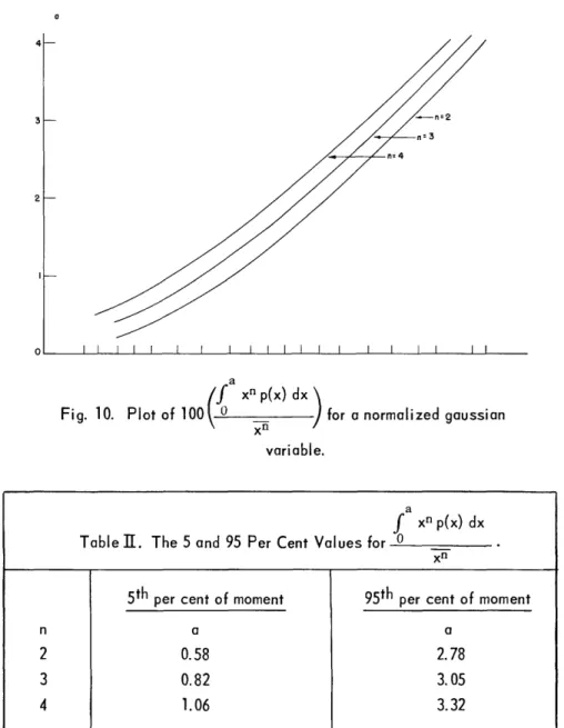
°ey/

y

t CHARACTEII'.-', ' 3 F L SB.ION

CHARACTERIZATION

OF PROBABILITY DISTRIBUTIONS

FOR EXCESS PHYSICAL NOISES

L

ON/J

TECHNICAL REPORT 276 SEPTEMBER 7, 1956

RESEARCH LABORATORY OF ELECTRONICS

MASSACHUSETTS INSTITUTE OF TECHNOLOGY CAMBRIDGE, MASSACHUSETTS

The Research Laboratory of Electronics is an interdepartmental laboratory of the Department of Electrical Engineering and the De-partment of Physics.

The research reported in this document was made possible in part by support extended the Massachusetts Institute of Technology, Re-search Laboratory of Electronics, jointly by the U. S. Army (Signal Corps), the U. S. Navy (Office of Naval Research), and the U. S. Air Force (Office of Scientific Research, Air Research and Develop-ment Command), under Signal Corps Contract DA36-039-sc-64637, Department of the Army Task 3-99-06-108 and Project 3-99-00-100.

MASSACHUSETTS INSTITUTE OF TECHNOLOGY RESEARCH LABORATORY OF ELECTRONICS

Technical Report 276 September 7, 1956

CHARACTERIZATION OF PROBABILITY DISTRIBUTIONS FOR EXCESS PHYSICAL NOISES

Jack Hilibrand

This report is based on a thesis that was submitted to the Department of Electrical Engineering, August 1956, in partial fulfillment of the requirements for the degree of Doctor of Science, Massachusetts Institute of Technology.

ABSTRACT

Theoretical and experimental techniques are described for characterizing the probability distributions of certain excess physical noises by their moments. Theo-retical methods are presented for applying this "moments technique" in the time domain to random-pulse noise, and in the frequency domain to any random functions for which the moments exist. The frequency-domain technique is used for a theoretical study of the approach to a gaussian distribution of random-pulse noise that is subjected to severe band-limiting. In contrast, the departure from a gaussian distribution of random-pulse noise that is band-limited by RC cutoffs at low and high frequencies is examined by using the time-domain technique. It is found that the approach of noise distributions to gauss-ian is governed by the "memory" of the filter system rather than simply by its band-width.

An experimental system is described for measuring the first four moments of noises in the 0.2 cps - 10 kc range. It is concluded that experimental measurements of moments are more desirable than direct probability density measurements when the goals are: (a) to categorize broadly the form of continuous noise distribution by a small number of parameters, and/or (b) when a minimum investment of time and equipment is desired.

Measurements on 1/f noise in germanium diodes confirm (within experimental error) that the first probability distribution of this noise is gaussian in nature. Some effects of limited system bandwidth are illustrated by measurements on the distinctly non-gaussian "avalanche" noise in silicon junction diodes.

Table of Contents

Page

I. Introduction 1

Excess Physical Noise 1

Noise Amplitude Distributions of Non-Gaussian Noises 1

Measurement of Amplitude Distributions 2

Results of this Investigation 2

II. The Moments Technique for Use in the Frequency Domain 4

Significance of Moments in Evaluating Amplitude Distributions 4

Evaluation of the Moments in the Frequency Domain 5

Evaluation of the Moments in the Time Domain for

Random-Pulse Noise 9

III. Some Applications of the Moments Technique 12

Evaluation of the Higher-Order Power Spectra for

Random-Pulse Noise 12

The Approach to a Gaussian Distribution of Filtered Random-Pulse Noise: An Application of the Moments Technique in the

Frequency Domain 17

The Effect of Low-Frequency Filtering on Random-Pulse Noise:

An Application of the Moments Technique in the Time Domain 22

IV. Semiconductor Noise Measurements 25

Measurements and Techniques 25

Errors Resulting from Length of Observation Time 27

Errors Resulting from a Limited Amplitude Range 31

Measurements of 1/f Excess Noise 33

Avalanche Noise 34

V. Conclusions 45

Acknowledgment 46

Appendix: Further Applications of the Moments Approach in the Time Domain 47

Bibliography 50

I. INTRODUCTION

1.1 EXCESS PHYSICAL NOISE

The noises that appear in electronic devices have been classified as thermal noise arising from statistical fluctuations of the thermal energy of the device, shot noise arising from the discrete nature of the electron, and excess physical noise (1), which includes all of the noises that derive from the particular physical structure of the

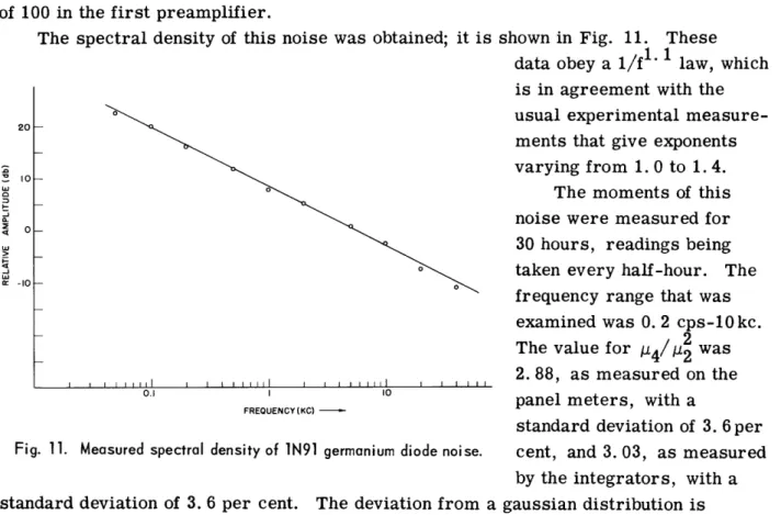
mate-rial, and which is usually ascribable to conductivity fluctuations. Some examples of excess physical noises are the 1/f noise in semiconductors, avalanche noise in the reverse breakdown of semiconductor diodes, and flicker noise in vacuum tubes. In this work the first-order amplitude probability density of 1/f semiconductor noise and of avalanche noise were investigated experimentally. We shall assume that the reader is acquainted with the standard results in noise theory, such as those that can be found in reference 12.

Direct measurement of the first probability density is difficult for physical noises that have a 1/f spectral density, since this spectrum leads to long correlation times and, therefore, to long observation times and elaborate data collection systems. Filtering the low-frequency components of the noise to decrease the correlation time, however, can modify the probability distribution considerably. It is for this reason that we have used a technique of measuring moments for the purpose of evaluating the probability distribution, rather than measuring the distribution density directly. Since one purpose of these measurements is to establish experimentally the gaussian or non-gaussian nature of semiconductor 1/f excess noise, proof is included that for a wide class of non-gaussian noise models, RC limiting of the low-frequency portion of the spectrum leads to an increasing deviation from a gaussian distribution. Studies undertaken for avalanche noise (which is markedly non-gaussian) illustrate some of the effects of filtering on the probability distribution that is to be measured.

1.2 NOISE AMPLITUDE DISTRIBUTIONS OF NON-GAUSSIAN NOISES

Two classes of non-gaussian noises have received attention recently: noise derived from gaussian by a resistive nonlinearity and noise resulting from the super-position of independent pulses.

In the past decade work has been done by Rice, Bennett, Middleton, and others (2), in examining the effect of a resistive nonlinear system on the probability distribution and spectral density of a gaussian noise input. The general problem of the effect of resistive nonlinearities on amplitude distributions of all orders is susceptible of im-mediate solution; therefore attention was focused on mathematical techniques for the evaluation of the power spectrum. Solution for the probability distribution in the case of nonlinearities with energy storage was accomplished, for a square-law detector fol-lowed by filtering, by Kac and Siegert (3), but other detector characteristics have not been treated analytically.

Random-pulse noise, which has been investigated by Rice and Middleton (4), provides a field in which application of the moments technique is straightforward. This report is devoted primarily to examination of pulse noise, although the methods used can be applied more generally (9).

1. 3 MEASUREMENT OF AMPLITUDE DISTRIBUTIONS

Early measurements (5) of probability distributions were made by inspection of photographic records of the waveforms under investigation. The accuracy of the results obtained by this method was usually limited by the length of the analyzed time interval, which, in turn, was limited by the laboriousness and time-consuming nature of the measurements. Later techniques have been based either on the use of electronic level selectors or on measurements made with cathode-ray tube displays (6). The electronic-selector technique, when combined with digital counting schemes, can provide measure-ments over the long periods needed for the tails of the distribution, but it requires extensive and complicated equipment. Measurements with cathode-ray tube displays and photocells are limited by the integrator time constant to moderate lengths of observation time. If photographic techniques are used to examine the display, the time of observation can be extended considerably, but the numerical evaluation of the probability density is quite difficult.

We have no specific knowledge, at this time, of any instance of the use of measurements of moments to evaluate waveform probability distributions, but the widespread use of this technique in statistical and actuarial work leads us to suppose that its application to (electrical) waveforms must have at least been contemplated by others.

1.4 RESULTS OF THIS INVESTIGATION

In this report analytic methods for evaluating the moments of a probability dis-tribution after filtering by using either a time-domain or frequency-domain approach are provided, together with examples of their application. A proof of the approach to a gaussian distribution for random-pulse noises, which are examined after severe band-limiting, is given. Attention in this proof is centered on the nature of the ap-proach to a gaussian distribution as the bandwidth is decreased. In contrast, the

effect of RC filtering of the low end of the random-pulse noise spectral density is found to be an increasing departure from a gaussian distribution, and consideration

of this case leads to a clarification of the concept of band-limiting which is implied in such a statement as "under band-limiting non-gaussian noises tend toward a gaussian distribution."

Equipment which has been used to measure moments experimentally is described briefly and the conditions under which experimental use of the method of moments is most desirable are discussed. The results of measurements on 1/f noise from a

germanium junction diode and on avalanche noise in silicon junction diodes are given.

Some of the effects of a limited-system bandwidth on measurements of a non-gaussian

distribution are shown by the results for filtered avalanche noise.

II. THE MOMENTS TECHNIQUE FOR USE IN THE FREQUENCY DOMAIN AND TIME DOMAIN

2.1 SIGNIFICANCE OF MOMENTS IN EVALUATING AMPLITUDE DISTRIBUTIONS In this section we shall show how the values of the moments define the first-order and nth-order probability distributions and how, in practice, the first-order probability density would be obtained from the values of the first-order moments.

The first-order probability density function p(x) and its characteristic function Fx(u) are uniquely related by the Fourier transformation:

Fx(u) = f ejUxp(x) dx (1)

p(x) =

1

2f -0

Equation (1) is also the definition of the characteristic function. The characteristic function can be written in the form of a Taylor series in which the coefficients of the terms are the moments of the probability distribution.

F.(u) = E (ju)' Xn (3)

n-0 n

It is clear, then, that the complete set of moments (if they exist) uniquely defines the probability density.

It is usually desirable to use only the lower-order moments (customarily, the first four moments), x, 2, x3 , and x4, to obtain the probability density. Two techniques are commonly used to provide an expansion of p(x) in terms of the moments. The earlier technique - the Gram-Charlier series and the Edgeworth expansion (7) - uses an expansion in terms of the gaussian distribution pg(x) and its derivatives in order to approximate slightly non-gaussian distributions. Pearson's system (8) is an attempt to fit both slightly non-gaussian and markedly non-gaussian distributions by using only the first four moments. It predicates a distribution density with a single extremum and a high degree of contact with the axis for large amplitudes. It is designed for use in fitting this wide class of density functions. We have found that the Pearson system is easy to use and that it usually provides a good fit to the continuous distributions we encountered (9).

The nth-order probability distribution, the nth -order characteristic function, and the expansion of the nth-order characteristic function in terms of the higher-order

auto-correlation functions are given by extension of the first-order equations.

P(U2. ( 2 .xn ) =

ff

fexp

F,,(ui, u21 U =

f

Fx(ul, U2, . Un ) (u o (iuU)l (x)"1j2) (xV2 (xn) n

vl=0 v2= =0 = vl! 2! vn

(6) A higher-order Edgeworth series may be used to approximate the probability density for almost-gaussian distributions by using higher-order autocorrelation func-tions( 10), but there is no higher-order equivalent to the Pearson system available. In this investigation attention is centered on the first-order distributions.

2.2 EVALUATION OF THE MOMENTS IN THE FREQUENCY DOMAIN

We now describe a technique for the evaluation of the moments and the higher-order autocorrelation functions of the output of a linear filter, in terms of the frequency response of the filter H(o) and the corresponding higher-order autocorrelation functions of the input variable. The relation for the moments was first stated by Mazelsky (11). We add the generalization to higher-order autocorrelation functions, together with a demonstration that as complete a characterization of the output variable as is avail-able for the input function can be provided.

Consider an ensemble of random functions x(t) which are statistically stationary and ergodic. These functions are passed through a linear network whose impulse

response is h(t) to yield the output variable y(t).

From network theory (12), the system function of the linear system, H(w), is defined as the Fourier transform of the impulse response.

h(t) - 1 f H(w) ei°tdo (

H () = f h(t) e-i()tdt (8)

The relations between the input and output of the system can be written in the time domain and frequency domain as

y(t) = f h(r) x(t - ) dr (9)

_ 00~~~~~~~~~~~~~g

and

Y () = H (o) X () (10)

where X(o) is the Fourier transform of x(t), and Y(w) is the Fourier transform of y(t)

in a sense that will be specified in Eq. (18).

The first autocorrelation function and spectral density will now be defined before

we proceed to the nth-order equivalents. The first-order autocorrelation function is

defined (13) by the relation

T

qx(r) = lim T 2T x(t) x(t + r) dt (11)

The Fourier transform relation defines the spectral density x(w) (also called the

power spectrum):

(D ( ) = f x (r) eji"rdr (12)

x r) =

f

By a direct extension of Eq. (11) we can define the nth-order autocorrelation

function as

~bx(rl, r2, .. rn) = lirm 21 x(t) x(t + r1) x(t + r2) ... x(t + rn) dt (14)

The existence of this function for all values of r 1,

2, . . .

, T

can be demonstrated

for all time functions that would be encountered in physical measurements. The

restriction to physically realizable waveforms implies that x(t) must remain finite at

all times. Then all the moments of x(t) will exist. Since the maximum value of

x(T, T₂, . ,Tn) (which occurs for O = T1 = T = Tn) is the (n + 1)th

moment of x, then Ox(T, T2, . . rn) will always exist.

The corresponding n -order spectral density is defined by the multiple Fourier

transform relationship:

(xD (c o 2.. n) = rff

'.

(15)

O~x (l, 2, * rn) =(2-)

rr

Jx

(

xn+l=

x(

=Ox

This relation implies that x(01 W2, 2' ' ' ' ' n) is integrable and hence can have no singularities worse than delta-functions.

There is another property of the nth-order spectral density which we shall

establish: an expression for the spectral density in terms of the Fourier transform of the time function X(w). If we define the sectioned variable xT(t) as being equal to x(t) in the region from -T to +T and zero elsewhere, we can write the Fourier transform of x(t) as

XT () = (f XT (t) exp(-jct) dt) (18)

where < f(t) > indicates the ensemble average of f(t). From Eq. 15, we have

'x0,2-- 2T

2 n[T lim TfrXT(t) I xT(t+rl).. xT(t+rn)dt)1

X exp[-j (& 1rl ₊ 2r2 + ...+ rn)] drl dr2 . . . drn

Tim 2T([Ir XT(t+ rl) exp[-j _x(t+rl)]drl f XT(t + r2) exp[-o₂(t + r2)]dr₂

T-oo 2T [

-[f xT (t + r) exp [-j on (t + rn)] drn| [ xT(t)exp[j ( + 2+ + n)t] dt

Therefore,

D.X(o1, w' 2 n) = im 1 XT(cl1) XT(O2)... XT(&n) XT(W1+ c2+ ... + +n) (19)

T 2T

which, in general, contains delta-functions, but is integrable in w-space. Next we evaluate the (n + 1) th-order moment of y(t):

yn+l = lim [y(t)]n+l dt (20)

T-,oo 2T -T

We can substitute for y(t) from the convolution equation(Eq. (9)).

n+

lim

[r

1

T.-o 2T -T [oo J

ff ..fh(o)h(a ₂)... h(an+) do₁ d2 ... dn+l

x lim

1

T-,- 2T -T

ff

f

= WIh(f) h(a₂). h(an+l) [-)

r

x exp i [ (1- a2) + w2 (al1- a3) +- + (l- On+l)] dw do2 . . dn] da da2 . . . dan+

yn+l = (+)n

ff"

....

~L)~.

%n)H

x H*(o,1 + 2 + . + n) dol do 2 . . .don

In the light of Eqs. (19) and (10), this relation indicates that we could have written more simply:

yn+l = I

r

r

f

2 7 - -T - 2T x dw, d 2 . . .dO n

(l ff 0 .flim 1 [XT)XT(₁ XT(2) . . . XT ( n ) XT (O1 +2+ ... On)]

x [H((w,) H((02) . . H(n) H* ( 1 + 2 + . + n) ] d ₁ d ₂ . . . d _n

which yields the same result. It is clear that in general the nth-order spectral densities of the input and output of a linear system are related by

Qy(Ol, 2 ... ' On) = x(Ol' On) H(to)H(o2 . 2).. H(on)H* (o + t2 + .. + On)

(22)

The existence of this relationship means that given the nth-order autocorrelation function or the nth-order spectral density of an arbitrary random function which is the input to a linear filter, we can obtain that autocorrelation function or spectral density of the output which is of the same order. This technique, then, provides as much

information about the output of the linear system as we know about the input. Our attention, it should be emphasized, is fixed on the autocorrelation functions and the power spectra rather than on the probability densities. This is permissible, since the probability densities are uniquely defined by the autocorrelation functions.

It must be noted that the application of these techniques to any actual problem is quite complicated and that, in general, machine computation would be required. The characterization of a distribution may be quite approximate, however. Frequently, one is interested only in the first-order probability density or the first- and second-order distributions. For these limited goals, the moments technique is useful.

2.3 EVALUATION OF THE MOMENTS IN THE TIME DOMAIN FOR RANDOM-PULSE

NOISE

For the class of random functions that consist of the sum of a series of pulses whose initiation times are randomly distributed, Middleton's simple and direct

technique (14) enables us to obtain the moments in the time domain. We shall use this technique to examine the effect of linear systems on the moments only, but the higher-order autocorrelation functions can also be obtained from Middleton's equations.

The proof of the Middleton relations presented here is simpler than that provided by Middleton (15) because we are interested only in the first-order characteristic func-tion.

Consider a function xK(t) which consists of the sum of K randomly occurring pulses in an interval (0, T), and for which K itself is a random variable with a Poisson distri-bution. Then we can write

K

xK(t) = E ake(t- tk; rk) (23)

k=l

where ak is the amplitude coefficient of the kth pulse, rk is a duration coefficient for the kth pulse, and tk is the occurrence time of the kth pulse. K, ak, rk, and tk are independent random variables for which the probability density functions are p1(K),

P2(ak), P3(rk), and p4(tk), respectively. The characteristic function of a single pulse can be written:

F

(u) =

(24)

Since the pulses are independent of each other, the characteristic function of the

random variable x(t) can be obtained, using the Poisson nature of p

(K), as

9

~

- K

Fx

(u)

p

(K)

Fx

(u))

K=O k=l

= E(NT)K exp(-NT) [F (u)]K K=0 K!

= exp [- NT + NT F (u)]

where N is the average number of pulses per second.

Fx (u) = exp NT +NT f exp [juak e(t - tk; rk)] P2(ak) P3(rk) P4(tk) dak drk dtk

-0 0 0

= expNTf f T [ exp[jua_ke(t - tk _; rk)] - 1] P2(ak) P3(rk) P4(tk) dak drk dtk}

The assumption of a random pulse initiation time in the interval (0, T) means that p4(tk) = 1/T for 0 < tk < T and zero elsewhere. If we assume that the duration of the pulses is short compared with T, we can extend the upper limit of integration for tk

to infinity. Let us further assume that the pulse parameter distributions are the same for all pulses.

Then

F,(u) exp{ N r ff [exp [juae(t -tk; r)] -1] 2(a) 3(r) da dr dtk}

Since the process is assumed to be stationary, we can set t = 0. We also substitute p = -tk to obtain the final form:

Fx(U)

Let us apply this expression to the particular case in which p2(a) = 6 (a - a),

P3(r) = 6 (r - ro), e(p, r) = 1, for 0 < p < r and zero elsewhere. Therefore,

Fx(u) = exp{N fr0 [exp(juao) - 1]dp}

= exp [N r(exp(juao) - 1)] (26)

This is the characteristic function for a Poisson distribution (16); therefore, we

can write

c(a) writ ]x/ exp(-Nro) X n) n = 0, 1, 2,... (27)

o

exr

)!

x

n)

Usually, the evaluation of Fx(u) in closed form and the subsequent Fourier trans-formation are not feasible. In such cases, it is usually possible to obtain the semi-invariants and moments.

The semi-invariants or cumulants are defined (17) by the equation

M1 m

F,(u)

[

(28)

We can put Eq. (25) into this form by using the series expansion for the exponential function, which yields

F.(u) = expN

f

= exp

{

[

Therefore,

Km = N fo f amem(p;r) p2(a) p3(r) da dr dp (30)

This expression can usually be evaluated, and the nth-order moment can then be obtained from the nth-order semi-invariant (17).

The use of this time-domain technique permits us to examine the effects of various network configurations and parameters on a type of non-gaussian noise that appears frequently in models of noise processes. The effects of a variety of networks are examined in the appendix.

11

III. SOME APPLICATIONS OF THE MOMENTS TECHNIQUE

The relations established in Section II for the moments in the time domain and frequency domain will now be applied. The frequency-domain techniques will be used

in examining the nature of the approach to a gaussian distribution for random-pulse noise which is sharply band-limited as the bandwidth goes to zero. Section 3. 1 is devoted to establishing the nature of the higher-order autocorrelation functions and spectral densities. The effects of band-limiting will be considered in section 3. 2. In section 3. 3 we shall consider the effect on the distribution of eliminating the low-frequency energy in random-pulse noise, and illustrate the application of the moments technique in the time domain.

3.1 EVALUATION OF THE HIGHER-ORDER POWER SPECTRA FOR RANDOM-PULSE NOISE

The complete expressions for the first-, second-, and third-order spectral densities of random-pulse noise will now be presented, and the nature of the terms in the general nth-order spectral density will be discussed. It should be pointed out that this is actually the same random variable that was treated in section 2. 3, the initial assumption made here, that all the pulses are identical, being removed by a suitable averaging technique later in the development.

We consider a random function of time x(t) which is the sum of a series of randomly occurring pulses, all of which have the same waveform. The sectioned function exists only in the interval (-T, T), where T is very much greater than the

individual pulse length, and can be written

N

xT(t) = E f(t-t n ) (31)

n=1

where tn is a random variable with a uniform distribution in the interval (-T, + T). The average pulse density is N = <N/2T>. Since the individual pulses exist only for a length of time small compared with T, the usual autocorrelation function of an

individual pulse goes to zero in the limit as T--~co. In this section, therefore, we shall use a modified nth-order autocorrelation function, (71, Tf 2, ... , Tn), for the

individual pulse, which is defined by:

f(r'1, r₂.... n) f

f=

The modified spectral density is defined as the Fourier transform of f (1, 2, ... , n) It can then be shown that

Df ( ₁, (C2 . .. ) F(o1) F (c2) . . . F (n) F* (o + 2 + · · ·+ n )

(33)

12

where

F () = f f(t) exp (-jet) dt (34)

Instead of the mean value of f(t), we shall use

f

= f

f(t) dt = F(O)

We shall now examine the first-order autocorrelation function of x(t).

=T°) 2T T ft - tm )1 f(t- tn + r)J dt (35)

T~

2Tn=1

We distinguish two separate cases here: where n = m and where it does not.

(r)

=

l

f(t-

t

f(t-

t +r)

f(t-

t

f(t

- t

+

dt

T-00

2T

m

nj

(36)

m-n

The first term is merely the modified autocorrelation function of an individual pulse and thus it yields

lim N"f(r) = N f(r) (37)

T- 2T (37)

In evaluating the second term we recall that the initiation times are independent random variables with probability density 1/2T in the interval (-T, +T) and zero elsewhere. The contribution from this term must be a constant, since, on an ensemble basis, the probability of overlap of the pulses f(t- ta) and f(t - tb + T) is independent of T. If the displacement between the initiation times of the two pulses, ta -tb + , lies in the interval (td, td + dtd), then the contribution from this term will be

(f(td) =

f

The probability that the displacement time will be within this interval is dtd/2T. There are N(N-1) such contributions in the second term. Therefore, the value of the second term is

lim 1 N(N

1)

T-0o 2T -T 2T T- (2T)2

= lim N(N-1) f2 = 22 (39)

T -.- (2T)2

We can see this result more directly by noting that the first term contains all of the contributions from pulses overlapping with themselves, while the second term contains all of the contributions from random overlapping with the other pulses. For

13

two statistically independent random variables, the mean of their product is the product of their means: The mean of each variable is N f; therefore, the contribution from the second term should be N2 2. Both of these trains of logic will be employed freely in the development of the higher-order autocorrelation functions.

The expression for the autocorrelation function of a sum of identical randomly-occurring pulses of density N pulses per second thus becomes

O5x ( r ) = Nf(r) + 2 (40)

Fourier transformation of this result yields the first-order spectral density

x(6o) = ±Nf(w) + 2r j22 (o) (41)

Next, we consider the second-order autocorrelation function.

x (r, r2) = T f(t-

t

Three cases can be distinguished here: all of the indices are identical; one index differs from the other two; all three indices differ.

When all of the indices are identical:

T N N

lim

1

f(t-ti) f(t-t

+

r

f(t-tj

+

r2)1

dt

Tim

1

Toc 2T -

1=1

T-_ 2T=1

= N

f(7

r,

2)

If one index differs from the other two, we get three possible terms:

TimN

N

rnlim

f

[f(t

- t)

f(t

- t + r

) f(t

-

+

2)

+

f(t - t) f(t

-

tm

+ r)

f(t

- t + r2)

T

2T

mri

X/_lm1

+ f(t

t)

f(t

t + r

)

f(t - t+

r2)dt

We consider the first of these terms and then generalize the result, thus obtaining

a complete expression for the case in which one index differs from the other two.

T N N

T

2T

f

E

[f(t-t )

f(t-tf,

r

dt

'- _ m=1

We notice first that the values of these terms must be constant with respect to 2,

since t and tm are independent random variables. If we define f(t - t)f(t - t + r

)

as a new variable g(t - t ), we can apply the same reasoning that we used for the

second part of the first-order autocorrelation function, and thus obtain

14

lim 1 N(N T -.oo 2T T T 1) f f g(t-t ) f(t-tj -T -T = lim [N(N T-o 2T = N2 f(rl

f,

2T

T

t

f(t

Generalizing from this result, we see that the terms in which one index differs from the other two are equal to

N2f [f(r _{1 )} + f(r _{2 )} + f(r - r2)_]

The case in which all three indices are different requires application of the same techniques. We have T N lim 1 T-,o 2T -T _=1 N N E

E

f(t

- te)

f(t

-

t

+ r

-

r

The result will be a constant, since tQ, tm, and tn are independent random variables. Consider the situation in which t - tm + 1 lies in the interval (tdl, tdl + dtdl) and tQ - tn + 2 lies in the interval (td2, td2 + dtd2) for tdl and td2 within the interval

dtdl dtd2 (-T, T). The probability of this situation arising is

(2T)2

The value of the integral of the product at this point is f (tdl, td2). There are N(N-1)(N-2) possible ways in which this can occur. Therefore, for the third case, we find:

lim I N(N - 1)(N - 2) T f(td) dtd1 dtd2 _=

N3

T--- 2T T -T 2T 2T

= N3 f3

Therefore, the second-order autocorrelation function can be written:

x(rlr2 ) = Nf( rl,r2) + N2 [f(rl ) + + (f(r2) _{_} r2)] + 3 3]f(r (43)

The second-order spectral density is evaluated by a Fourier transformation: (x (a 1,W2 ) = N f(01,(62) + 2 N 2_f[5f(l)& ( 2) + f (2) (&1) + f( (1) 8( + 1+ 2)] + (2 7)2N3f3 8(61) $(02) (44) 15 + td) dt dtd] Therefore

The third-order autocorrelation function can be found by an extension of these methods. X(r1,r2,r3) Tim

2T

II

x

[m_f(t-tm+ 2)] [l

f(t-tn

r3]dt

Here we can distinguish five cases: (1) all of the indices are identical, (2) three of the indices are identical and one differs, (3) the indices are identical in two pairs which differ from each other, (4) two indices are identical but the other two differ from this pair and from each other, and (5) all of the indices differ. Now we can obtain the correlation function by the same procedure that was used earlier, and we find (listing the results for the five cases in the proper order) that:

x (rlr2r_{3 )} = N f(rl,r2,r_{3 )}

+ N2f[gf(rl,r2) + f(rl,r 3 ) + SCf(r2,r3 ) + f(r2- rlr 3- rl)

+ N2 [f(rl) f(r3 - 2 ) ) ) + f(3-+ f(r3)f (r2- rl)] (46)

+ N3 f2[ 1 ) + +f(r 2 ) + f(3r + f(r 3- r2 ) + f(73 3 + + - ff(r(r2rl)]

+ N4 j4

The usual Fourier transformation leads to the corresponding third-order spectral density. (x(01,02,c~_{3 )} = Nif(o01,2,03) + 2r N2f [f(c)₁ , 2) 6()3) + )f(&)1,C)3) 6()2) + f()2,)3) $5(1 ) + f(6 2,( 3)8(6)1 + 22 + + 3)] + 2trN2[Df(6l) f( 3)(W 2 + 0)3) + Df( (2)(f(03)(1 + 3) + Pf(63) f(2) 8( ₁+ 02)1 (47) + (2 tr)2 N3f2 [~f (6 $ w2) (3) + f() f () (o) 5(3) + ()f (3) $(wl1) $(o02 ) + f (6₃) (01) ((02 + 0)3) + ff(0 3) 8() 2) 6(01+ 03) + )f (02) (0w3) 6(01+ 02)] + (2 r)3 N4 4 (1) 8(02) 8(6o3)

The generalization of this technique to nth-order autocorrelation functions and spectral densities is rather lengthy, but possible. It is usually sufficient, however, merely to note the nature of the various terms of which these functions consist.

16

---We first consider the nth-order autocorrelation function. ---We must consider n + 1 indices. Let us take the case in which the indices are equal in groups of ml, m2, ma so that m + m2 + .. .1.. + ma = n + 1. The spectral-density terms that

correspond to this situation will be of the form

[4)ff(t"t 2 .... m 1

X fml0ml+l ml+m2-1)(om + oml+l + + oml+m2) ] x

[f (tom l+m2+.. +ma.' oml+m2+...+ma.l+1 .. w On-l1) (48)

X '8(t+m 2+... +ll +lWm+m 2+...+mal+l + ... + . + +

On)]

This general expression will be of considerable use in section 3. 2 in which we examine the nature of the approach to gaussian statistics when this type of noise is band-limited.

We have now developed the first-, second-, and third-order autocorrelation func-tions and power spectra for a function that is the sum of identical random pulses of density N pulses per second. In addition, we have examined the general characteristics of terms in the nth-order spectral density.

The extension of these results to the case in which the pulses are not identical but are determined by the values of some parameters, '1, 2' ' ' ' ' b' whose joint

probability distribution, P(i₁, 2' .'.' b)' is known, canbe found by use of the relation

ff(

. ..

rn·

ffJ

0

since the pulses are still independent of each other.

3.2 THE APPROACH TO A GAUSSIAN DISTRIBUTION OF FILTERED RANDOM-PULSE NOISE: AN APPLICATION OF THE MOMENTS TECHNIQUE IN THE FREQUENCY DOMAIN

We can now present a proof of the approach to a gaussian distribution of random-pulse noise when it is passed through a narrow-band filter with abrupt cutoff limits. While the usual proof by the Central Limit Theorem (18) is applicable to this type of noise, the proof by the moments technique provides additional information about the nature of the approach to a gaussian distribution - and especially about the way the odd moments vanish as the bandwidth is reduced. This proof provides an example of the application of the moments method in the frequency domain. Other examples of applications of this technique are given in reference 9. We shall consider the first four moments in detail to illustrate the technique and then discuss the nature of the approach to a gaussian distribution of the higher-order moments.

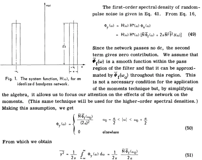
Let us consider an idealized bandpass network for which H(w) has the form shown in Fig. 1. Since no dc is passed by this network [H(O) = 0] it is clear that the mean of the output distribution will be zero.

17

H(w)

Fig. 1. The system function, H(6), for an

idealized bandpass network. I

the algebra, it allows us to focus our att

moments. (This same technique will be

Making this assumption, we get

N

0

The first-order spectral density of

random-)ulse noise is given in Eq. 41. From Eq. 16,

D y(o) = H(o) H*(o) x(()

= H(o) H*(6o) L[Nf(o) + 2 N2f2a(o)] (49)

Since the network passes no dc, the second

;erm gives zero contribution. We assume that

Af(w) is a smooth function within the pass

region of the filter and that it can be

approxi-mated by Of(wo) throughout this region. This

Ls not a necessary condition for the application

of the moments technique but, by simplifying

ention on the effects of the network on the

used for the higher-order spectral densities. )

o - a < (o < 0 + a

02 2

elsewhere (50)

From which we obtain

Y _

1

= 1

2r -- 2 r 2 a

(51)

If we examine the second-order spectral density in Eq. (44), we see that we can

immediately eliminate most of the terms. All terms which include the function 6 (w

),

6(w2), or 6(w

+ w

) give zero contribution to the third moment of y(t), since H(ol),

H(o

), and H*(w

+ w

) are involved in the evaluation of y

.

The one remaining term

is N- f(rol,

2

Therefore,

(P (o1,( 2 ) = Nf( 1l,6 2) H(61) H(6)2) H*((o1 + 2)

(52)

Since y3 equals the integral of this function in the ol, w

plane, let us examine the

regions in this plane for which the function is nonzero. In Fig. 2a we consider the

narrow-band case in which a < 2/3 wo and in Fig. 2b we consider the situation in

which a > 2/3 oo. It can be seen from Fig. 2a that there are no regions in which

the product H(CO

) H(w

) H*(w

+ w

) is nonzero. The third moment is always zero

for a < 2/3 co. From Fig. 2b it can be seen that the total area of the region of

overlap is 3 (3. 2)o)2= 27 (a 2

18

I

fig. 3. The volume centered at (, o0, - 0) in which the function H(o1) H(0 2) · H(e 3 )

- H* ( + °)2 + 3) is nonzero.

NON-ZERO REGIONS ARE SHADED

Fig. 2. Nonzero regions in the wl- 2plane for the function H(o_l) H(o2) ·H* (1l+ 2).

From this value we find that

3

i

)1 \2

3 t 2 (2 a)3

O for a < 2 3

27 (a _ 2 )

This sharp cutoff of the third moment at a = 2/3 w0 is the result of the idealization in

the infinitely sharp cutoff of the network but it does provide information about the region of rapid approach to zero of the third moment for more realistic networks. Examination

of the situation for the higher-order odd moments will provide an extension of this insight into the nature of the approach to a gaussian distribution.

Next we examine the third-order spectral density given by Eq. (47). If we elim-inate the terms that incorporate 6 (w1) 6 (w(), 2), 6(w3) or 6 (w1 + w2 + w3), we are left with

O (1,Cj23) - [H(61) H(62) H(` 3) H*(61 + 2 + °63)]

x N f(cDli2,6)3) + 2N 2 [ ) f(l) f ( 3) 8(62+ c63)

+ f ( 2 ) Of(6)3) (o1 + 6)3) + (f(O63) f(c 2 ) (01 + o2)]

(54) 19 2( o (a) a < _$ Wp 3 rnIcuJ 1io . a __-o\ .-for a > 2 o 3 (53) I

\

_

L

_I

\

Consider the contribution to y4 from the first term in this function: N f(w1l02,X3 ) H((1) H(O2) H(03) H*(o1 + co2 + 03)

Corresponding to the wl, w2 plane in the evaluation of the third moment we now have

w1, 2, 3 space in which we must find the volume in which H(w)) H(w2) H(w3)

H*(01 + w2 + 3) is nonzero. For H(wol) H(wO2) H(w3) there are eight cubes with sides

of length ac centered at the eight points specified by ( woo, ± o, ± W0o). When the

further requirement that H*() 1 + 2 + o3) be nonzero is added, the cubes at

(+ 0 o', + 0, +o) and (- 0o, - w0 , -) are eliminated and the other six cubes are reduced in volume. The solid that remains at (o, 0, - )o) 0 is shown in Fig. 3. The

volume of the solid is a3/2. It should be noted that if of(W1 w2' 3) takes on the

value 0f(wo, -wo, w0) throughout the volume centered at (wo, -wo, w0), it will take

on this value within each of the other five solids because Of (O, -0), o) F*w o ) F F (o)o (o) F*(F*( o )

Therefore, this first term in the third-order spectral density of the contribution 1 3 N f (o' 0o' ) ) to y .

3 16a

Examination of the symmetries involved in the second term in shows that three equal results will be obtained. Therefore, we now first of these three terms. We seek to evaluate

input gives a

cy(Wl' 2' 3)

consider only the

1(.3 .ff 27?N2 f(Cl) )f(<3 ) (&)2+ 3 ) H(w1 ) H(&J2 ) H(co3 ) H*( 1+ 2+ co3 )d d dow 3

Integration with respect to w2 yields

()2 ) ; f(6il) Ff(o3) H(o 1) H* (w3) H(oj3) H*(wl) d d 3

2T" ff - f01o'()3c

which reduces to

O f(2ao ) ] 2

[ r

Now, we can write for the fourth moment:

y4= 3N Of(COO,-o0, _{O0 ) + 3 N f(ro)]2}

(2 r)3(16 a) 2

2a

The skewness and excess (19) are

(55) 2 TN [f(_o)]3/2 (a

)

tO

and

=

_

Y2- (y2)2

8r

N

Next we examine the behavior of the nth-order moments, considering the behavior for n even and n odd separately.

The moment of order n (for n even) will be derived from the n-l th-order auto-correlation function.

x(12 rn. lim

f

E

f(tt

=

[ia

f(t

-tm

rl)]

f(

T~,~ 2T m (-tm ' l f(t-t

(58) There are, then, n indices to be considered. If there are any cases in which a single index differs from all the others, a 6 (

w

form of the term in Eq. (48). If we multiply this by H(wl) ... H(wn ) H*(wl +... +wn l) and integrate with respect to the n-lth variables, we obtain a result of the order of

l/aa. Since our interest centers on the normalized nth moment, which is n/(1,2) n / 2

n/2

(n/2)-a

and is of the order n a /2, we must consider the behavior of /) . This will be a constant for a = n/2, which implies that when the number of different indices is equal to n/2, there is a contribution to yn which is independent of a. Since no indices may appear less than twice, this specifies that, for a--O, the only terms in ox(wl... Wnl)

that contribute are those of the form

[f (6o1)] [f(63) (62 + 60₃)][f (5) 8(6)4 + 65)] . [f (0n-) 8(on-2 + on-1) ]

The number of such terms is equal to the number of different selections that can be made among n indices, taken two at a time, and it equals (n-l)(n-3)... 5- 3- 1, which is precisely the value of the normalized gaussian nth moment. The terms of next higher order in a will have (n/2)-l different indices (all appearing twice except one which appears four times). They will make a contribution to the normalized moment of order a and will go to zero directly with the bandwidth. Other terms will be of higher order in a up to a(n/2)-1 for the case in which all indices are identical.

Next consider the nth-order normalized moment, where n is odd. There are n indices in this case but since every index must appear more than once, there can, at most, be (n-l)/2 different indices. This would yield a term of order

2 \2

a - coo 2w

3 _{which exists only for} 2O

a > . The term of next higher order

(3/2 3

21

I---_2

O

5( 2w

is of order and will be nonzero for a > . We can describe t

a5/2 5

stain

th

2

tth

situation for the n moment as a increases from zero. When a - , the nth

n n-1

moment becomes nonzero. It now increases proportional to n/2 W ;he

{hen 2 0

a reaches the value , another series of terms comes into existence which is of n-2 n-3

order

n-2

This process continues until a > , when all the non-dc 3

terms will have appeared. It is clear, then, that however narrow we make the band-width, some higher-order odd moments will exist.

This application of the moments technique in the frequency domain has shed some light on the nature of the approach to gaussian statistics with narrow-band filtering, in addition to providing a proof of this approach to supplement the usual Central-Limit-Theorem proof.

3.3 THE EFFECT OF LOW-FREQUENCY FILTERING ON RANDOM-PULSE NOISE: AN APPLICATION OF THE MOMENTS TECHNIQUE IN THE TIME DOMAIN The effect of an RC low-frequency filter on the amplitude distribution of a sum of random pulses can be found by evaluation of the moments in the time domain. The result will have significance for the question of how much of the low-frequency energy of a physical noise process can be filtered out if we are interested in determining the form of the amplitude probability distribution of a physical (possibly non-gaussian) noise.

We take, as a particularly iluminating example of a noise process, a train of unit steps with Poisson-distributed starting times. We seek information about the amplitude probability density of the output from a linear filter whose system function is

H(s) = 1

( ros ) ( ) (59)

This system function corresponds to the filtering imposed by a typical measuring sys-tem whose response falls off at 20 db per decade both at high and low frequencies. We shall allow T to vary while To is held fixed so that for T < o we have a constant

frequency cutoff and a variable high-frequency limit, while, for r> o' it is the low-frequency cutoff that is variable.

The response of this network to a unit step is

e(t) = r (e-t/ r - e't/O) (t > 0) (60)

It should be noted that H(s) is unity for the middle-frequency region, if is the low-frequency pole (T > To), but is not unity, if T is the high-frequency pole. We shall consider the normalized moments, however, so that this will make no difference in our results.

We use Eq. (30) to establish an expression for the mth semi-invariant.

K_m = N f [e(t)]m dt (61)

0

Performing the indicated integration, we obtain the general expression:

mN (_l)rm! (62)

=m F(r\)ri

z=

We evaluate the first four semi-invariants (17) and obtain from them expressions for the skewness 1 and the excess y2 which will be examined in greater detail.

K1= N K NT2 K = 2N r3 2 ( + r) 3(r + 2 )(2r0 + ) K4 = 4(ro + r)(3 r + )(r + 3 ) K3 1 1 K2 3(r + 2 r)(2r + r) 4 \2 ( + )3/2 (63) K4 1 1 Y2 K2 N (3 r + r)(rO + 3r) (64) 3 (r0 + r)

The skewness and excess are plotted in Fig. 4. It is clear that it is the low-frequency pole which modifies the probability distribution of the sum of Poisson-distributed unit steps most markedly. Furthermore, as the system eliminates an increasing portion of the low-frequency energy, the distribution deviates increasingly from gaussian. This indicates the need for clarification of any broad statement which maintains that: as the bandwidth in which a non-gaussian noise is examined goes to zero, the amplitude prob-ability distribution goes to gaussian. This statement does not apply in the above case because the skirts of the system function are not sharp enough. Evidently some property of the skirts must be included in the "band-limiting" statement.

23

0.9-43 .0.865 .7F=, 0.977 N- Ny0 \__ 0.0819 0.819 S-PLANEiS-PLNE 000977 0.977 POLE AT I/r IS HIGH- POLE AT I/r IS LOW- Nto r

FREENCY CUTOFF FREOUENCY CUTOFF

, , , I,,,,1 , I ,,, ENCY , I I I I, I , I , ,,, , ,,,,

0.01 0.1 1.0 10 101

T/T

-Fig. 4. Effect on the skewness and excess of moving a pole of H(s).

The necessary clari-fication can be obtained by restating the criterion for approach to a

gaus-sian distribution as fol-lows: For a progressively longer filter memory, a filtered non-gaussian noise approaches a gaussian distribution. By limiting the low-frequency response in the manner considered in the example above, we actually reduce the mem-ory of such a nonoscil-latory system. Middle-ton (14) points out that the amount of overlapping in a sum of random pulses provides a good criterion for the deviation from a gaussian distribution. This viewpoint is certainly reasonable on the basis of Central-Limit-Theorem ideas, and it evidently applies to the case of pulses modified by passing through a linear network. In that case, the amount of overlapping at the output clearly becomes a function of both the overlapping of the original input pulses and the memory of the filter.

In relation to experimental methods of measuring the probability distribution of noises for which the sum of randomly occurring pulses is the model, it is clear from the foregoing that "eliminating the low-frequency energy" can often lead to measure-ments that are farther from gaussian than is the actual noise distribution.

24 u,, w 2ft w u (nx NC Xw --- ---

~ ~~~~~~~

IV.

SEMICONDUCTOR NOISE MEASUREMENTS

4.1

MEASUREMENTS AND TECHNIQUES

The nature of the measurements of 1/f noise in germanium junction diodes and

of avalanche noise in silicon junction diodes will now be discussed and an estimate of

the expected error in these measurements provided. A brief description of the

moments-measurement equipment is given here; for a more complete description

see reference 9.

Four measurements were made on semiconductor noise:

1. The second, third, and fourth moments were evaluated experimentally.

2. The frequency spectrum was measured between 100 cps and 60 kc.

3. Photographs of the noise waveforms were taken.

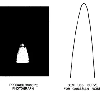
4. Probabiloscope photographs were taken to provide a qualitative picture of the

distribution density.

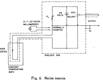
The measuring system is shown in Fig. 5.

The noise source consisted of

INISE

TAI.

I

TEKTRONIX TEKTRONIX NOISE _ PREAMPLIFIER VARIABLE PREAMPLIFIER SOURCE TYPE 122 ATTENUATOR TYPE 122

ANALYZER

constant temperature bath and a

suit-ANALYZER able biasing circuit. This noise

source is shown in Fig. 6. For the

TYPE OSCILLOSCOPE

1N91 diode, measurements were made

PHOTOGRAPHY

at room

constant

temperature bath in this case was

TYPE 304A one

pint of water in a Dewar

FAR PRARARII nA -. ma e r

SCOPE Since measurements were taken

I

every half hour, it was felt that the

low thermal heat transfer into the Dewar flask would result in temperature variations

so small that the moments measurements would not be affected. Application of

Newton's law of cooling to available data (20) gives an expected change of 0.1°C for a

5°F temperature differential over one-half hour. The silicon diode noise was

meas-ured at the equilibrium temperature of a mixture of dry ice and acetone. This mixture

in a Dewar flask provided a constant temperature environment.

The noise spectrum analyzer (21) is a heterodyne analyzer with filter bandwidths

of 10 cps and 100 cps. It provides continuous measurements of the noise spectrum

between 100 cps and 60 kc.

A Tektronix 535 oscilloscope and a 35-mm oscilloscope camera were used to

photograph single stroke traces of the noise. The brightness of the oscilloscope spot

was increased in proportion to the rate of travel by an intensifier as described by

Kemp (22).

I I lh nrhhilnrtesno 19R. 1,lc d

a DuMont 304A oscilloscope with a

5ADP15 tube, a 35-mmoscilloscope

camera, and an optical wedge with

a density range of 1:3 (a fractional

transmission range of 1000:1). No

attempt was made to evaluate

numerically the probability

dis-tribution, since the intention was

to obtain a qualitative picture of

CONSTANT % AL LI.A LLLJJL L _L4J PLl L J.D LJL

TEMPERATURE

BATH

with

result from the moments.

Fig. 6. Noise source. The moments analyzer (Fig. 7)

consisted of an

amplifier-rectifier-cathode-follower unit which fed three function generators whose outputs were

propor-tional to the square, cube, and fourth power of the noise. Three integrators then

provided the desired moment values.

The amplifier-rectifier-cathode-follower unit provided a gain of approximately

eight from a paraphase amplifier so that the second Tektronix preamplifier would not

operate in a nonlinear region. It was found simpler to design a full-wave rectifier to

feed the square- and fourth-powe; function generators than to design function generators

with the desired accuracy of balance. The full-wave rectifier was balanced to 1 per

cent. The cathode followers in this unit had output impedances of the order of 100 ohms.

The frequency response of these units was good at 40 kc.

The function generators used back-biased diodes to match straight line segments

to the desired power laws. The desired accuracy was 2 per cent of the desired value

over output amplitude ranges of 50:1, 125:1, and 256:1 for the square-, cube-, and

fourth-power units. They are dc units so that the minimum amplitudes in these

ranges are set by the function-generator drift and the drift of the integrator input

cir-cuit. The frequency response of the over-all function-generator system, including the

amplifier-rectifier-cathode-follower unit, is good to 10 kc.

The integrators were designed to average the input function with a 10-second time

constant, and then apply this average to

drive watt-hour meters. The only limita- INTEGRATOR A.x2

tion on the length of the integration period

is the

drift of

input circuits.

CATHODE-FOLLOWER the ease of taking readings every

half-hour (and resetting the zero) led us to do so

FUNCTION GENERATORS

in this study. In a half-hour period, the

over-all moments analyzer drift was less Fig. 7. Moments analyzer.

26

than 10 mv at the input to the chopper circuit in the integrator. The accuracy of the integrators is of the order of ±3 per cent except for very small inputs.

4.2 ERRORS RESULTING FROM LENGTH OF OBSERVATION TIME

In addition to the errors in measuring the moments inherent in the particular types of function generators and integrators that were used, there are unavoidable errors caused by the limited observation time and by the limited amplitude range that can be incorporated in the function generators. The limited observation time is particularly significant when an attempt is being made to measure the amplitude probability distribu-tion of noise with a 1/f spectral density, owing to the long correladistribu-tion times that are required.

Consider an ensemble of stationary ergodic random functions. We want to measure some property of this ensemble by observing one member of it for a period of time T. If we performed this operation on each member of the ensemble, we would obtain a series of values that are random functions. We want to estimate the variance of these values in order to determine how accurately a measurement that is made on one member represents the average value for the ensemble. In the limit T--co the value for one member must approach the average value for the ensemble (from the ergodic

property). For the case of 1/f noise, we shall be interested in measuring the moments of a random function which, it develops, actually has a gaussian or near-gaussian distribution. For such distributions, the contribution to the measured average from extreme values increases as we consider higher-degree moments. Therefore, we would expect to find that a longer observation time is required for the fourth moment than for the second, and, indeed, this is true. The development of the results below is based on a theory of statistical errors in measurements on random time functions developed by Costas (24), Davenport, Johnson, and Middleton, (25), and Siegert (26). We wish to measure the average value of a function of a random variable, x(t). Let us define z(t) as

(t) = g [x(t)] (65)

We are, then, interested in the properties of

M(T)

I

T o

In this study we shall examine the mean and the variance of M(T), using the method described in reference 25.

The ensemble average is

M(T)

-

-

T o

This is expected, since the ensemble is stationary. The variance of M(T) is

2 (T) = 2 ( - r ( 2] d r (68)

Now consider the evaluation of 0 z(T) for the first four moments in terms of

For z = x we see immediately that

z (r) = x ( (69)

For z = x w e w i s h t o e v a lu a t e z2z x x 2, where x1 = x(t) and x2 = x(t +

r).

We now specify that x(t) obey a gaussian distribution law. Although this limits the

results somewhat, they still can serve as a guide for the case in which x(t) is nearly

gaussian. We can, from Eq. (6), write

x x2 - (j)4 Fx(Ul,u2) ] (70)

xx- du u

J2:u2

For a gaussian distribution,

Fx(u1,u2

,

We take x = 0, since the equipment used in this investigation did not pass dc. If we

perform the indicated operation on Fx(ul, u

), we obtain

z(r) X2 2 a + 2 2(r) (72)

We can use the same technique in order to get the correlation functions of the other

moments. We list the results for the second, third, and fourth moments:

x2 (r)= 2 ()+ x (73)

3(t) = 6 () + 9 ox ,(r) x (74)

Ox4(r) = 244x(r) + 72x2 () + 9 (75)

Consider first the simple case in which

, x(r) = e Irl/' (76)

This is the case for which

x() = 2 ax

'0 2 + 1 (77)

0

where or 2 is the ensemble-wise variance of x(t).

X 2 2 2 2

Now we can obtain values for arx(T), a ₂(T), 3(T), and a 4(T) from Eq. (68). We

assume T >> T.o Then we obtain x x x

a2 (T) = 2 0 o,2 (78) T U2 (T) 20 4 o2₂(T) - 2Torx (79) o2 (T) - 22 T ° (80) 2 4(T) 84 o0 x

T

We have now obtained two properties of the distribution of the first four moments of a sample taken in time T: the mean and the variance. It is clear that z(t) = [x(t)]n does not have a gaussian distribution. However, the operation of integration for a

period T can be thought of as passing [x(t)]n through a filter whose memory is T. This, as we have seen in section 3. 3, leads to an approach towards gaussian statistics at the output of such a filter. To a good approximation, therefore, we can assume a nearly gaussian distribution of the sample statistics. If M(T) obeyed a gaussian distribution, the probability of a single value lying within the 2aM limits would be 95 per cent. We can establish a criterion for a suitable observation period, T, then, on the basis that

2_{aM = 0. 05M.}

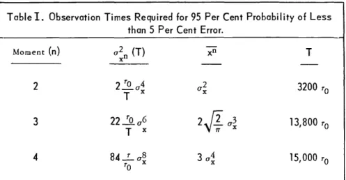
In Table I expressions for a 2n (T), x, and the value for T, using this criterion

xn r/

for the case when the autocorrelation function x(7) = ax e ,are given. For the third moment, we have substituted I x3l (the third absolute moment) for x3 _{so that the}

criterion can be applied.