Calibration of the CMS drift tube chambers and
measurement of the drift velocity with cosmic rays
The MIT Faculty has made this article openly available.
Please share
how this access benefits you. Your story matters.
Citation
Chatrchyan, S. et al. "Calibration of the CMS drift tube chambers
and measurement of the drift velocity with cosmic rays." Journal of
Instrumentation 5 (March 2010): T03016 © 2010 IOP Publishing and
SISSA
As Published
http://dx.doi.org/10.1088/1748-0221/5/03/T03016
Version
Original manuscript
Citable link
https://hdl.handle.net/1721.1/121948
Terms of Use
Creative Commons Attribution-Noncommercial-Share Alike
CMS PAPER CFT-09-023
CMS Paper
2010/01/13
Calibration of the CMS Drift Tube Chambers and
Measurement of the Drift Velocity with Cosmic Rays
The CMS Collaboration
∗Abstract
This paper describes the calibration procedure for the drift tubes of the CMS barrel muon system and reports the main results obtained with data collected during a high statistics cosmic ray data-taking period. The main goal of the calibration is to deter-mine, for each drift cell, the minimum time delay for signals relative to the trigger, accounting for the drift velocity within the cell. The accuracy of the calibration pro-cedure is influenced by the random arrival time of the cosmic muons relative to the LHC clock cycle. A more refined analysis of the drift velocity was performed during the offline reconstruction phase, which takes into account this feature of cosmic ray events.
∗See Appendix A for the list of collaboration members
1
1
Introduction
The Compact Muon Solenoid (CMS) [1] is a general-purpose detector whose main goal is to explore physics at the TeV scale, by exploiting the proton-proton collisions provided by the Large Hadron Collider (LHC) [2] at CERN.
CMS uses a right-handed coordinate system, with the origin at the nominal collision point, the x-axis pointing to the center of the LHC, the y-axis pointing up (perpendicular to the LHC plane), and the z-axis along the anticlockwise-beam direction. The polar angle, θ, is measured from the positive z-axis and the azimuthal angle, φ, is measured in the x-y plane.
The central feature of the Compact Muon Solenoid apparatus is a superconducting solenoid, of 6 m internal diameter, providing a field of 3.8 T. Within the field volume are the silicon pixel and strip tracker, the crystal electromagnetic calorimeter (ECAL) and the brass/scintillator hadron calorimeter (HCAL). Muons are measured in gas-ionization detectors embedded in the steel return yoke. In addition to the barrel and endcap detectors, CMS has extensive forward calorimetry.
The barrel muon system [3] is divided in five wheels. Every wheel is composed of 12 sectors,
each covering 30◦in azimuth, as shown in Fig. 1.
Figure 1: Schematic representation, in the x−y plane, of the chamber positions within a wheel
of the muon barrel system of the CMS experiment. The labels and the numbers of the muon stations are shown. Because of mechanical requirements, the top and bottom MB4 sectors are split in two distinct chambers.
Each sector contains four stations equipped with Resistive Plate Chambers (RPC) and Drift-Tubes (DT) chambers. The four DT chambers are labeled MB1, MB2, MB3, and MB4 going
2 1 Introduction
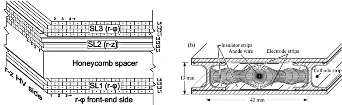
DT chambers. The chambers are interleaved with the steel return yoke of the magnet and are composed of three groups, called “super-layers” (SL), of four staggered layers of independent drift cells, for a total of about 172 000 channels. A schematic representation of a chamber is shown in Fig. 2 (left).
The chamber volume is filled with a Ar(85 %)/CO2(15 %) gas mixture, kept at atmospheric
pressure. Two of the super-layers have the wires parallel to the beam direction and measure the rφ coordinate, the other super-layer has wires perpendicular to the beam direction and measures the z coordinate. The chamber provides a measurement of a track segment in space. The outermost station is equipped with chambers containing only the two rφ super-layers. The basic element of the DT detector is the drift cell, illustrated in Fig. 2 (right), where the drift lines and isochrones are represented. All chambers were operational, fully commissioned, and the number of problematic channels were less than 1 %.
The DT system is designed to provide muon track reconstruction, with the correct charge as-signment up to TeV energies, and first-level trigger selection. It also yields a fast muon iden-tification and an accurate online transverse momentum measurement, in addition to single bunch-crossing identification with good time resolution. The good mechanical precision of the chambers allows the track segments to be reconstructed with a resolution better than 250 µm [3].
A fundamental ingredient of the DT system is the calibration, which is used as input to the local hit reconstruction, within the drift cells, and thereby influences the precision of the track reconstruction. This paper describes in detail the DT calibration procedures, to obtain reliable calibration constants, and presents results obtained from the extensive commissioning run with cosmic ray events performed in Autumn 2008, the Cosmic Run At Four Tesla (CRAFT) [4], in preparation for LHC running.
2.5. The Muon System 35
10 11 12 1 2 3 4 4 13 5 6 7 9 8 1 2 3 5 6 7 8 9 10 11 12 14 x y MB3 MB4 MB2 MB1
Figure 2.13: Numbering of stations and sectors.
Figure 2.14: Section of a drift tube cell.
the boundary of the cells and serve as cathodes. I-beams are insulated from the planes by a 0.5 mm thick plastic profile. The anode is a 50 µm stainless steel wire placed in the centre of the cell. The distance of the track from the wire is measured by the drift time of electrons produced by ionisation. To improve the distance-time linearity, additional field shaping is obtained with two positively-biased insulated strips, glued on the the planes in correspondence to the wire. Typical voltages are +3600 V, +1800 V and -1200 V for the wires, the strips and the cathodes, respectively. The gas is a 85%/15% mixture of Ar/CO2, which provides good quenching properties and a saturated drift velocity, of about 5.4 cm/µs. The maximum drift time is therefore∼ 390 ns, i.e. 15 bunch crossings. A single cell has an efficiency of about 99.8% and a resolution of ∼ 180 µm.
Four staggered layers of parallel cells form a superlayer, which provides the
Figure 2: Left: Schematic view of a DT chamber. Right: Section of a drift tube cell showing drift
lines and isochrones. The voltages applied are+3600 V for wires,+1800 V for electrode strips,
and−1200 V for cathode strips.
The data sample used for the calibration process and the trigger conditions are summarized in Section 2. The main characteristics of the DT calibration process are described in Section 3. The process consists in the determination of the inter-channel synchronization, described in Section 4, the analysis of noisy channels, treated in Section 5, and the calculation of the time pedestals and the drift velocity, described in Sections 6 and 7, respectively. The DT calibration workflow, including the monitoring of the conditions, is performed within the CMS computing framework, as described in Section 8. Finally, a more refined analysis of the drift velocity in the muon system, within the offline reconstruction process, is presented in Section 9.
3
2
Cosmic Ray Event Trigger and the Data Sample
The long cosmic ray data taking in 2008 with and without magnetic field allowed a detailed study of the DT drift properties and an improved understanding of the calibration constants. About 270 million events were collected with a 3.8 T field inside the solenoid magnet. In this configuration, the radial component of the magnetic field in the DT chamber positions does not exceed 0.8 T.
The DT system was the primary trigger source for most of the collected events. The local trigger [3] was designed to operate with collisions taking place at the center of the CMS detector, and it is performed searching the φ-matching of hits in each chamber. This is achieved using dedicated hardware, which configures the expected track paths from one chamber to another. Due to the different origin, direction, and timing of the cosmic rays, as compared to muons from proton-proton collisions, dedicated adjustments were needed to properly configure the DT trigger for high efficiency during CRAFT. This required relaxing the extrapolation algo-rithm with a particular configuration of the DTTF (DT Track Finder) as explained in more detail in Ref. [5]. Therefore, during data-taking with cosmic rays, the L1 trigger was generated by the coincidence in time of two segments in two stations of the same sector, or adjacent sectors, and a rate of about 240 Hz was provided to the Global Muon Trigger.
About 20 million events, out of the 270 million collected during CRAFT, were used for the calculation of the calibration constants. They have been chosen from stable runs where most of the DT system was operational. No quality cuts are, in principle, necessary to perform the calibration. However, in order to have a clean sample of muons, a transverse momentum cut of 7 GeV was applied.
3
The Calibration Process
Charged particles crossing a DT cell produce ionization electrons in the gas volume. The de-termination of the relationship between the arrival time of the ionization signal and its spatial deposition is the primary goal of the calibration task, which leads to the extraction of the drift times and drift velocities.
The arrival time of the ionization signal is measured using a high performance Time to Digital Converter (TDC) [6]. This is the main building block of the read-out boards of the DT system. It is a multi-hit device in which all hits within a programmable time window, large enough to accommodate the cell maximum drift time, are assigned to each Level 1 Accept trigger. The drift time is directly obtained from the time measured by the TDC, after subtracting a time pedestal which contains contributions from the latency of the trigger and the propagation time of the signal, within the detector and the data acquisition chain. The first goal of the calibration procedure is, therefore, to determine the time pedestals, as described in Section 6. The expected precision of the time pedestal calibration during the cosmic ray data-taking is limited by the arrival time distribution of cosmic rays which is flat within the clock cycle and it is of the order
of 25 ns/√12.
The other relevant quantity for the DT calibration process is the effective drift velocity. It de-pends on many parameters, including the gas purity and the electrostatic configuration of the cell, the presence of a magnetic field within the chamber volume, and the inclination of the track. The parameters connected to the working conditions of the chambers are monitored continuously [3]: the high voltage supplies have a built-in monitor for each channel; the gas is at room temperature and its temperature is measured on each preamplifier board inside the
4 4 The Inter-Channel Synchronization
chamber; the gas pressure is regulated and measured at the gas distribution rack on each wheel, and is monitored by four further sensors placed at the inlet and outlet of each chamber. The adequacy of the flow sharing from a single gas distribution rack to 50 chambers is monitored at the inlet and outlet line of each individual chamber. A possible leakage in the gas line can be sensed via the flow and/or the pressure measurements.
Five small gas chambers, one for each wheel, are used to measure the drift velocity in a volume of very homogeneous electric field, located in the accessible gas room adjacent to the cavern, outside of the CMS magnetic field. Each of these chambers, called Velocity Drift Chambers (VDC) [7, 8], is able to selectively measure the gas being sent to, and returned from, each in-dividual chamber of the wheel thus providing rapid feedback on any changes due to the gas mixture or contamination. During the CRAFT data-taking period only one such chamber was used.
No noticeable variation of the parameters described above is expected among different regions of the spectrometer. However, the magnetic field and the track impact angle may vary substan-tially from chamber to chamber, as they occupy different positions in the return yoke.
Two methods for calculating the electron drift velocity in a DT cell are presented here. They both assume a constant drift velocity in a given chamber. The first method, discussed in Sec-tion 7, is based on the measurement of the effective drift velocity using the mean-time tech-nique, which computes the velocity value at the super-layer granularity level. The second method, discussed in Section 9, relies on the muon track fit, which determines track-by-track the time of passage of the muon and the drift velocity as additional free parameters of the fit, together with the track position and inclination angle. The assumption of a constant drift ve-locity is considered a good approximation because the magnetic field in the chamber volume is usually low and approximately homogeneous. A third method based on a parameterization of the drift velocity as a function of the drift time, the magnetic field, and the muon trajectory is discussed in Ref. [9].
The detailed drift velocity analysis, described in Section 9, also reveals non-linear effects in the innermost stations (MB1 chambers) of the barrel external wheels (Wheel +2 and Wheel -2), where the strongest radial magnetic field component, of about 0.8 T, is present.
The DT calibration process also depends on the different signal path lengths to the read-out electronics (called inter-channel synchronization time) and on the list of noisy channels, as will be described in the following sections.
4
The Inter-Channel Synchronization
The inter-channel synchronization is calculated for each read-out channel of each chamber, in order to correct for the different signal path lengths of trigger and read-out electronics. This is a fixed offset, since it only depends on cable/fiber lengths, and it does not need to be re-calibrated very often. Nevertheless, it is useful to frequently redo its calibration, to monitor the correct behavior of the front-end electronics. The inter-channel synchronization is determined by test-pulse calibration runs. The design of the data acquisition system allows such runs to be taken during the normal physics data-taking, by exploiting the collision-free interval of the LHC beam structure, called “abort gap”.
During special calibration runs, a test-pulse is simultaneously injected in four channels of a front-end board, each one from a different layer of a super-layer, simulating a muon crossing the super-layer. To perform the scanning of the entire DT system in only 16 cycles, the same
5
test-pulse signal is also distributed to other four-channel groups, 16 channels apart.
The so-called t0 calibration consists in determining, for each DT channel, the mean time and
the standard deviation of the test-pulse. In the calibration procedure, the events are split in two samples: the first is used to compute the average value, within a full chamber, of the signal propagation time from the test-pulse injector to the read-out electronics; the second is used to calculate, for each individual channel, the difference between the time of its test-pulse signal and the average value of the chamber.
10 20 30 40 50 60 t0 [TDC Counts] -10 -5 0 5 10 15 CMS 2008 SL1 10 20 30 40 50 -10 -5 0 5 10 15 SL2 Wire Number 10 20 30 40 50 60 -10 -5 0 5 10 15 SL3
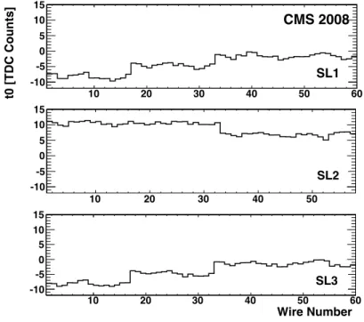
Figure 3: Inter-channel synchronization constants calculated from a test-pulse run. The results are shown for three representative layers, belonging to each of the three super-layers of cham-ber MB3 in Sector 9. The step-function shape reflects the grouping of channels among different front-end boards.
Figure 3 shows an example of a distribution of t0 constants for representative layers of the
three super-layers of a chamber, as a function of the channel number. The other layers show
very similar t0values. The t0 synchronization correction is always below 10 ns (1 TDC count
corresponds to 0.78 ns). The standard deviation is about 1 ns, for all channels. This is com-patible with the precision of the electronic chain. These corrections correspond to the distance between the front-end boards, located inside the chamber volume, and the read-out boards. Wires connected to a given front-end board belong to cells adjacent to each other, in the super-layer, and have approximately the same distance up to the read-out boards. This leads to the step-function shape seen in Fig. 3, more pronounced in the super-layers 1 and 3.
5
Noise Analysis in the DT Chambers
On the basis of systematic studies performed during several commissioning phases of the DT detector, a cell is defined as noisy if its hit rate at operating voltage, counting signals higher than a common discriminator threshold of 30 mV, is higher than 500 Hz.
6 5 Noise Analysis in the DT Chambers
Noise Rate [Hz]
0 1000 2000 3000 4000 5000 6000 7000 8000 9000 10000Number of wires
1 10 2 10 3 10 4 10 5 10B=0 - all subdet
B=3.8T - all subdet
B=3.8T - no(CSC+RPC+PIX)
CMS 2008
Figure 4: Distribution of the cell noise rate for different data-taking conditions: with and with-out magnetic field; with and withwith-out Cathode Strip Chambers (CSC), Resistive Plate Chambers (RPC), and Pixels (PIX).
The number and geometrical distribution of noisy DT channels have been studied, in particular, during a commissioning period without magnetic field and having the detector wheels sepa-rated from each other. In this section we describe the results of the noise analysis performed using the cosmic ray events collected during CRAFT. With respect to runs using random trig-gers, the noise analysis based on normal data taking runs has the advantage of reflecting the detector operation in more realistic conditions.
The first aim of the noise studies is to check the stability of the number of noisy cells in different conditions of the CMS detector. For all runs analyzed, the number of noisy cells is around 0.01 % of all DT channels. The rate of noise hits per cell is shown in Fig. 4, for a number of representative runs, with and without magnetic field, and with different sub-detectors included in the acquisition. The number of cells with a hit rate higher than 500 Hz is very small. Detailed information on the noise rate observed for representative runs, with different configurations of CMS detectors included in the data acquisition, is shown in Table 1.
An average noise rate of ∼ 4 Hz is observed in the DT system, essentially insensitive to the
magnetic field and to the status of nearby sub-detectors. In addition, it has been observed that around 50 % of the noisy cells remain noisy for long data-taking periods.
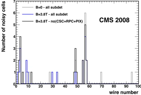
Studies have also been made concerning the position dependence of the noisy cells, within wheels and chambers. As seen on Table 1, most of the noisy channels are located in the in-nermost chambers (MB1), where the internal cabling is more complex, because of the reduced space. In Fig. 5, the noisy cell distribution is shown as a function of the wire number. The noisy cells appear concentrated in the regions of the super-layer close to the wire boundaries, which are different depending on the number of wires present in each chamber type (about 50
7
Table 1: Number of Noisy Cells in each chamber type (MB1, MB2, MB3, MB4) and average noise rate for some representative runs of different data-taking conditions. The results from the CRUZET (Cosmic RUn at ZEro Tesla) commissioning period are also shown, for comparison.
Data B Field Excluded Number Number Number Number Mean
Period [T] Sub-Det. Noisy Noisy Noisy Noisy Noise Rate
Cells Cells Cells Cells
in MB1 in MB2 in MB3 in MB4 [Hz] CRUZET 0 CSC, PIX 12 2 2 0 3.96 CRAFT 0 0 13 3 2 3.80 CRAFT 3.8 13 3 1 2 4.15 CRAFT 3.8 CSC 12 7 0 8 4.23 CRAFT 3.8 CSC, 17 5 0 0 4.50 PIX, RPC
for MB1, 60 for MB2, 70 for MB3, and 90 for MB4). The peaks also reflect the position of the connectors distributing the HV inside the super-layer, which generate some electronic noise in their proximity.
wire number
0 10 20 30 40 50 60 70 80 90 100
Number of noisy cells
0 1 2 3 4 5 6 7 B=0 - all subdet B=3.8T - all subdet B=3.8T - no(CSC+RPC+PIX)
CMS 2008
Figure 5: Number of noisy channels as a function of the wire number, for the data-taking peri-ods mentioned in Table 1. Each distribution corresponds to a different run and shows the noisy cells observed for chamber types MB1, MB2, MB3 and MB4.
The observed fraction of noisy cells (0.01 %) and the average noise rate (∼4 Hz) in the full DT
system are too low to affect the digitization efficiency or the trigger rate. It is important, how-ever, to exclude the noisy cells in the calibration process described in the following sections.
8 6 The Time Pedestal Calibration
6
The Time Pedestal Calibration
6.1 Computation of the Calibration Constants
The time pedestal calibration is the process which allows the extraction of the drift time from
the TDC measurement. For an ideal drift cell, the time distribution coming from the TDC (tTDC)
would coincide with the distribution of drift time (tdrift), and would have a box shape starting
from a null drift time, for tracks passing near the anode, up to about 380 ns, for tracks passing near the cathode.
Experimentally, some non-linear effects related to the electric field distribution inside the drift cell have to be considered in the response of these cells; they are enhanced by the track incli-nation and by the presence of the magnetic field. In addition, different time delays, related to trigger latency, and different cable lengths of the read-out electronics, also contribute to the
TDC measurements. The time measured by the TDC, tTDC, can be expressed as
tTDC =t0+tTOF+tprop+tL1+tdrift , (1)
where
• t0is the inter-channel synchronization used to equalize the response of all the
chan-nels at the level of each chamber, as described in Section 4;
• tTOF is the Time-Of-Flight (TOF) of the muon, from the interaction point to the cell,
in the case of collision events. In the case of cosmic events, this quantity cannot be defined because the time pedestal is an average of the arrival time of cosmic muons relative to the clock cycle;
• tpropis the propagation time of the signal along the anode wire;
• tL1is the latency of the Level-1 trigger;
• tdrift is the drift time of the electrons from the ionization cluster to the anode wire
within the cell.
The main goal of the calibration is the calculation of the time pedestal, ttrig, which is dominated
by the time delay caused by the L1 trigger latency:
ttrig=tTOF+tprop+tL1 . (2)
The value of ttrigis extracted for each super-layer directly from the tTDC distribution, referred
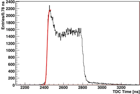
to as Time Box, after subtracting the noisy channels and correcting for the inter-channel syn-chronization. Figure 6 shows a Time Box measured during a CRAFT run, for one super-layer.
The value of ttrig is the turn-on point of the Time Box distribution. It is computed by fitting
the rising edge of the distribution to the integral of a Gaussian function, as illustrated by the continuous line in Fig. 6. The procedure is applied at the super-layer level and is described in more detail in Ref. [10].
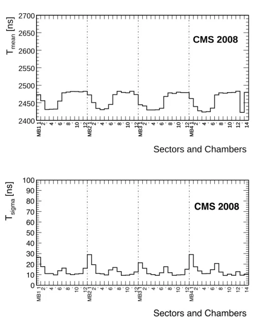
The main quantities calculated by the fit are the inflexion point of the rising edge, Tmean, and
its standard deviation, Tsigma, which represents the resolution of the measurement. Figure 7
shows the distributions of Tmean and Tsigma measured, in a CRAFT run with B = 3.8 T, for
the innermost rφ super-layer of a representative wheel, as a function of chamber type and sector. Similar results were obtained for the other wheels. Approximately constant values are observed for chambers of the same type and for all the wheels. The periodic structure seen in
6.1 Computation of the Calibration Constants 9 TDC Time [ns] 2200 2400 2600 2800 3000 3200 Entries/0.78 ns 0 200 400 600 800 1000 1200 1400 1600 1800 2000 2200 2400
Figure 6: Distribution of the signal arrival times, recorded by the TDC, for all the cells of a single super-layer in a chamber, after the cell-to-cell equalization based on the test-pulse calibration. The continuous line indicates the fit of the Time Box rising edge to the integral of a Gaussian function.
the Tmeandistribution, Fig. 7 (top), reflects the time-of-flight of the cosmic muon from the upper
sector to the lower sector. Indeed, the events contributing to the calculation of Tmeanand Tsigma
can be triggered by the upper or lower sectors. The events triggered by the top (bottom) sectors may also be detected by other non-triggering sectors, having a less precise time pedestal and, consequently, leading to a less precise determination of these quantities. Different runs during the entire CRAFT period have been analyzed, and a stable performance of the whole DT system has been observed. As expected, no dependence on the magnetic field strength was observed. The time resolution distribution, Fig. 7 (bottom), indicates the precision which the calibration
procedure can reach with cosmic rays. A standard deviation of ∼ 10 ns is observed for all
super-layers in all wheels, except in the vertical sectors, where the number of events is limited and the muon crossing angles are large. The time resolution precision is limited mainly by the random arrival time of cosmic muons relative to the clock cycle. Furthermore, the resolution in Sector 1 is systematically worse than in Sector 7 because the trigger cables that distribute the Level 1 accept signal are longer and, therefore, generate larger skews in the signal transmission.
After the determination of Tmeanand Tsigma, the time pedestal, ttrig, is estimated as
ttrig =Tmean−k·Tsigma . (3)
The k factor is evaluated by minimizing the position residuals, using the local reconstruction of track segments within chambers. After a few iterations, a k factor of 0.7 was computed for the CRAFT data and was applied to all super-layers. The position residuals were then recalculated and a final correction to the time pedestals was computed dividing the remaining offsets observed in the residual distributions by a constant drift velocity (54.3 µm/ns). The
10 6 The Time Pedestal Calibration
Sectors and Chambers
MB1 1 2 . 4 . 6 . 8 . 10. 12 MB2 1 2 . 4 . 6 . 8 . 10. 12 MB3 1 2 . 4 . 6 . 8 . 10. 12 MB4 1 2 . 4 . 6 . 8 . 10. 12 . 14 MB1 1 2 . 4 . 6 . 8 . 10. 12 MB2 1 2 . 4 . 6 . 8 . 10. 12 MB3 1 2 . 4 . 6 . 8 . 10. 12 MB4 1 2 . 4 . 6 . 8 . 10. 12 . 14 [ns] mean T 2400 2450 2500 2550 2600 2650 2700
CMS 2008
Sectors and Chambers
MB1 1 2 . 4 . 6 . 8 . 10 . 12 MB2 1 2 . 4 . 6 . 8 . 10 . 12 MB3 1 2 . 4 . 6 . 8 . 10 . 12 MB4 1 2 . 4 . 6 . 8 . 10. 12 . 14 [ns] sigma T 0 10 20 30 40 50 60 70 80 90 100
CMS 2008
Figure 7: Mean (top) and standard deviation (bottom) of the fitted inflexion point of the Time Box rising edge, for the innermost rφ super-layer for a representative wheel. The triggering sectors (3, 4, 5 and 9, 10, 11) are synchronized among each other. The sectors with vertical chambers (sectors 1 and 7) detect much less cosmic ray muons, leading to a poorly defined rising edge and a less accurate calibration.
6.2 Validation of the Calibration Constants 11
6.2 Validation of the Calibration Constants
Once the ttrigconstants are computed, the calibration process proceeds with the validation step,
which consists in studying the effect of these constants on the reconstruction algorithm. The analyzed quantities are the residuals computed, layer by layer, as the distance between the hit and the intersection of the 3D segment with the layer plane. A complete description of the local reconstruction procedure is given in Ref. [11]. To correct for the propagation time along the wire, the reconstruction of the segment is done in a multistep procedure. First the reconstruction is performed in the rφ and z projections independently. Once two projections are paired and the position of the segment inside the chamber is approximately known, the drift time is corrected for the propagation time along the wire and for the TOF within the super-layer, and the 3D position is updated.
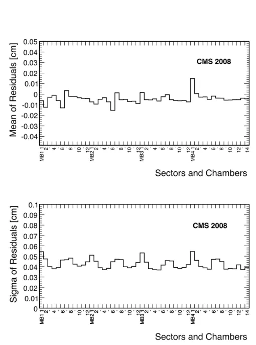
The mean values of the residual distributions calculated for the innermost rφ super-layer for a representative wheel are shown in Fig. 8 (top). A systematic offset with respect to the ori-gin is observed compatible with the systematic delay between the arrival time of the cosmic muon events and the clock cycle. The standard deviations of the fit to the residuals, shown in Fig. 8 (bottom) and in the range 400–600 µm, represent the spatial resolution obtained with the calibration process, a factor of two worse than the nominal resolution of about 250 µm [3]. The difference is caused by the spread of the muon arrival times inside the 25 ns time window associated with the L1 trigger. This dilution will not occur with LHC collision data.
7
The Drift Velocity Calibration
The aim of the drift velocity calibration is to find the best effective drift velocity in each region
of the DT system. In order to be consistent with the ttrigcalculation, described in Section 6, the
drift-velocity calibration is computed with a super-layer granularity.
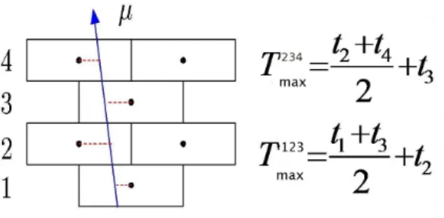
The calibration algorithm is based on the mean-time technique described in detail in Ref. [10].
In this method, the maximum drift time in a cell, Tmax, is calculated considering nearby cells in
three adjacent layers and using a linear approximation to determine the average drift velocity. As an example, Fig. 9 shows the simplest pattern of a muon crossing a semi-column of cells,
together with the equations used to calculate Tmax. In general, Tmaxdepends on the track
incli-nation and on the pattern of cells crossed by the track. Taking into account these dependencies,
a spread of about 28 ns has been observed in the calculation of Tmaxfrom CRAFT data.
The effective drift velocity can be estimated assuming a linear space-time relationship, veffdrift = Lsemi-cell
< Tmax>
, (4)
where Lsemi-cell=2.1 cm is half the width of a drift cell.
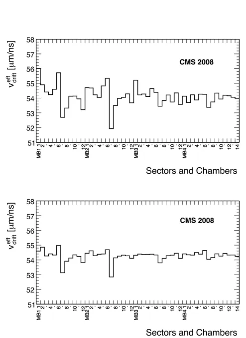
Drift velocities measured for each chamber/sector and for a representative wheel (other wheels give similar values) are shown in Fig. 10 for two CRAFT runs, one without (top) and one with (bottom) magnetic field. The drift velocity has approximately a constant value of 54.3 µm/ns, although with some systematic deviations, caused by limitations of the calibration procedure applied to cosmic ray events. As in the determination of the time pedestal, these uncertainties originate mainly from the random arrival time of cosmic muons relative to the clock cycle.
The ttrig uncertainty of about 10 ns, seen in Fig. 7 (bottom), corresponds to a relative
12 7 The Drift Velocity Calibration
Sectors and Chambers
MB1 1 2 . 4 . 6 . 8 . 10 . 12 MB2 1 2 . 4 . 6 . 8 . 10 . 12 MB3 1 2 . 4 . 6 . 8 . 10 . 12 MB4 1 2 . 4 . 6 . 8 . 10. 12 . 14 Mean of Residuals [cm] -0.04-0.03 -0.02 -0.01 0 0.01 0.02 0.03 0.04 0.05 CMS 2008
Sectors and Chambers
MB1 1 2 . 4 . 6 . 8 . 10. 12 MB2 1 2 . 4 . 6 . 8 . 10. 12 MB3 1 2 . 4 . 6 . 8 . 10. 12 MB4 1 2 . 4 . 6 . 8 . 10. 12 . 14 MB1 1 2 . 4 . 6 . 8 . 10. 12 MB2 1 2 . 4 . 6 . 8 . 10. 12 MB3 1 2 . 4 . 6 . 8 . 10. 12 MB4 1 2 . 4 . 6 . 8 . 10. 12 . 14 Sigma of Residuals [cm] 0 0.01 0.02 0.03 0.04 0.05 0.06 0.07 0.08 0.09 0.1 CMS 2008
Figure 8: Mean (top) and width (bottom) Gaussian parameters, as fitted to the distributions of the residuals between the reconstructed hits and the reconstructed local segments. The results are shown for the rφ super-layers for a representative wheel, after correcting the offset with respect to the origin of the residual distribution. Other wheels show similar results.
13
Figure 9: Schematic view of a super-layer section, showing the pattern of semi-cells crossed by
a track. The quantities ti in the equations represent the arrival time of the electrons within a
drift cell.
Fig. 10, meaning that the residuals calculated with the veff
driftand ttrigconstants do not represent
a significant improvement with respect to those shown in Fig. 8.
The drift velocity distribution measured in one of the VDC chambers (Section 3) during the full CRAFT period is shown in Fig. 11. An average drift velocity value of 54.8 µm/ns is observed, which is slightly different (0.5 % higher) from the one obtained from the DT data, mainly be-cause of the different shape of the electric field in the DT drift cell. The spread of the distribution is better than 0.2 µm/ns, and shows that no major variations occurred in the gas mixture or air contamination, during the entire data-taking period.
8
The Calibration Workflow and the Monitoring of the Calibration
Process
A fast calibration of the DT system is vital in order to provide the prompt data reconstruction with accurate calibration constants. The number of calibration regions is a compromise be-tween the need of keeping things simple, not requiring too large event samples, and the need of reducing systematic errors by separately calibrating regions where parameters may have very different values. As mentioned in previous sections, the super-layer granularity has been found to be the most suitable calibration unit.
In order to reach the precision obtainable with the fast calibration, about 104 tracks crossing
each super-layer are required. During LHC collision and cosmic ray data-taking periods, the calibration parameters have to be produced, validated, and made available for use in the re-construction within one day of data-taking. However, after the start-up phase, it is anticipated that at some point it will no longer be necessary to update the DT calibrations on a daily basis; on the other hand, they should be checked against a standard set in order to guarantee their stability.
cali-14 8 The Calibration Workflow and the Monitoring of the Calibration Process
Sectors and Chambers
MB1 1 2 . 4 . 6 . 8 . 10. 12 MB2 1 2 . 4 . 6 . 8 . 10. 12 MB3 1 2 . 4 . 6 . 8 . 10. 12 MB4 1 2 . 4 . 6 . 8 . 10. 12. 14 MB1 1 2 . 4 . 6 . 8 . 10. 12 MB2 1 2 . 4 . 6 . 8 . 10. 12 MB3 1 2 . 4 . 6 . 8 . 10. 12 MB4 1 2 . 4 . 6 . 8 . 10. 12. 14 m/ns] µ [ eff drift v 51 52 53 54 55 56 57 58 CMS 2008
Figure 10: Drift velocities computed using the mean-time method for a run with B= 0 T (top)
and for a run with B = 3.8 T (bottom). Results are shown for the rφ super-layers of each
15 m/ns] µ [ drift v 53 53.5 54 54.5 55 55.5 56 56.5 57 0 20 40 60 80 100 120 140 160 180 200 220 CMS 2008
Figure 11: Distribution of the drift velocity measured in one Velocity Drift Chamber (VDC) during the entire data-taking period.
bration workflow at a very early stage. A more detailed description of the overall CMS calibra-tion and alignment computing workflow used in the CRAFT exercise is given in Refs. [12, 13]. Within the CMS calibration and alignment workflow, particular selections of data, named Al-CaReco, were used. They contained a reduced number of events and a reduced event content, providing the minimal information to fulfill the requirements of the DT calibration task. The sample is saved at the CERN Analysis Facility (CAF) and taken as input to the calibration process. The calibration algorithm runs at the CAF and produces a set of constants, which un-dergoes a validation procedure before being copied to the central CMS database, where they become available to the CMSSW offline software framework.
The DT calibration workflow has been used also during the Computing, Software, and Anal-ysis challenge (CSA08), described in Ref. [12], which simulated with large event samples the conditions expected at LHC startup. This exercise simulated the production rate of the calibra-tion condicalibra-tions as it will happen during real collision data-taking. The long CRAFT data-taking period served as a thorough test of this workflow with the real detector.
The quality and stability of the calibration constants is a crucial part of the procedure and must be continuously monitored. Therefore, validation procedures have been set up within the central CMS Data Quality Monitoring (DQM) framework. A detailed description of the CMS DQM structure is given in Ref. [14].
Data quality assessment for the DT calibration constants consists mainly in defining the ac-ceptance criteria used to validate the constants, in the monitoring of time stability, and in the checking of continuous trends or sudden changes in operating conditions. The quality tests to assess the validation of the constants and to monitor their time stability are applied to the residual distributions calculated at the different steps of the calibration workflow. The compar-ison of the currently produced calibration constants with a reference set gives an indication of the stability of each particular calibration constant.
16 9 Drift Velocity Analysis
monitoring process, and for each of them detailed and summary DQM plots are provided. The DT condition constants have been monitored through the entire CRAFT data-taking period and have shown generally a good stability in time.
9
Drift Velocity Analysis
The drift velocity obtained with the calibration procedure described in Section 7 is derived from the measurements of the drift time and, as already mentioned, is limited by the uncertainty on the arrival time of the cosmic ray muons.
z[m]
Br[T]
MB1MB2 MB3 MB4 -0.4 -0.2 0 0.2 0.4 0.6 0.8 1 0 2 4 6Figure 12: Computed radial component of the magnetic field in the muon barrel chambers, for the different wheels, as a function of z.
A more detailed analysis of the drift velocity is presented in this section, taking into account the precise 3D space-time relationship for the hit reconstruction. In particular, it considers the influence of the magnetic field as a function of the position along the wire.
The presence of a radial magnetic field distorts the drift lines of the drifting electrons, because of the Lorentz force, resulting in a variation of the effective drift velocity. Figure 12 shows that the radial field component is not very high in the muon barrel chambers, except in the MB1 chambers of the outer wheels, closest to the endcaps. In these regions, the radial component of the magnetic field can be as high as 0.8 T, and changes significantly along the z axis, resulting in a variation of the effective drift velocity along the wire of each single cell, for rφ super-layers. The effect of the magnetic field has been studied in test beams with small prototypes [15], and more recently in the Magnet Test and Cosmic Challenge (MTCC), using cosmic rays in the CMS surface hall. These studies showed that the chambers maintain a good trigger and event reconstruction functionality, even in the most critical regions [16].
17
system is performed to determine the drift velocity. In the first step, a pattern recognition algo-rithm is applied to identify hits belonging to the same track. Once the hits have been identified, the track is reconstructed under the assumption of a 54.3 µm/ns nominal drift velocity. In the second step the track is refit treating as free parameters the drift velocities at each hit and the time of passage of the muon through the chamber. The method is applied to the rφ view of the track segment in one chamber, where there are eight measured points in most cases. The z super-layers, where only four points are available, at most, are less significant for this analysis. The drift velocity is taken to be the mean value of the track-by-track drift-velocity distribution.
Sector
2
4
6
8
10
12
m/ns]µ
Drift Velocity [
48
50
52
54
56
58
CMS 2008
Drift velocity from mean-time Wh+2 MB2 Drift velocity from fit Wh+2 MB2Figure 13: Mean values of the drift velocity for the MB2 chambers of Wheel +2, using the mean-time (squares) and fit (circles) methods. The differences between sectors when using the
mean-time method are due to ttriguncertainties that are not present in the fit method.
Figure 13 shows the mean values of the drift velocity for the MB2 chambers of Wheel +2, using the mean-time method described in Section 7 and the fit method described here. When using the mean-time method, the drift velocities have large systematic fluctuations from one sector
to the other. This is related to the errors on the ttrigdetermination described in Section 6, which
cancel when the fit method is used.
The average drift-velocity values from the fit method, for all the chambers, are shown in Fig. 14, for runs without and with magnetic field (of 3.8 T).
The data at B=0 T show an average value of 54.5 µm/ns for the drift velocity and a standard
deviation indicating that differences between chambers are in the order of 0.2 %. For B=3.8 T,
a second peak is observed at 53.6 µm/ns. This peak corresponds to the MB1 chambers of the
external wheels (Wheel +2 and Wheel−2) and is due to the presence of a higher radial magnetic
field.
Similar values of the drift velocity have been obtained using the same calibration procedure applied to the simulated pp collision data. These results, presented in Ref. [17], indicate that
18 9 Drift Velocity Analysis m/ns) µ Drift velocity( 51 52 53 54 55 56 57 58 59 # Chambers 0 10 20 30 40 50 60 70 80 90 CMS 2008 B=0 T Mean 54.51 ± 0.01 0.00660 ± Sigma 0.09697 m/ns) µ Drift Velocity ( 51 52 53 54 55 56 57 58 59 # Chambers 0 10 20 30 40 50 60 70 80 90 χ / ndf 2 3.287 / 4 Constant 6.812 ± 2.093 Mean 53.57 ± 0.03 Sigma 0.1244 ± 0.0308 CMS 2008 B=3.8 T Mean 54.49 ± 0.01 0.00674 ± Sigma 0.09319 0.03 ± Mean 53.57 0.0308 ± Sigma 0.1244
Figure 14: Drift velocities for B = 0 T (left) and B = 3.8 T (right). The small peak on the right
panel corresponds to the MB1 chambers of Wheel +2 and Wheel−2, and shows the influence
of a higher magnetic field in these regions.
the calibration algorithm delivers a more uniform response in the case of collision data and that a large fraction of the fluctuations observed in the drift velocity calibration from CRAFT data may be attributed to the topology and timing of the cosmic ray events.
CMS 2008
-150 -100 -50 0 50 100 150 m/ns] µ[ 5253 54 55 Wh-2 MB1 -150 -100 -50 0 50 100 150 Drift velocity 52 53 54 55 Wh-2 MB2 -100 0 100 52 53 54 55 Wh-2 MB3 -150 -100 -50 0 50 100 150 52 52.5 53 53.5 54 54.5 55 Wh-1 MB1 -150 -100 -50 0 50 100 150 52 52.5 53 53.5 54 54.5 55 Wh-1 MB2 -100 0 100 52 52.5 53 53.5 54 54.5 55 Wh-1 MB3 -150 -100 -50 0 50 100 150 52 52.5 53 53.5 54 54.5 55 Wh0 MB1 B=0T B=3.8T -150 -100 -50 0 50 100 150 52 52.5 53 53.5 54 54.5 55 Wh0 MB2 Local Z position [cm] -100 0 100 52 52.5 53 53.5 54 54.5 55 Wh0 MB3Figure 15: Drift velocities calculated using the muon track fit method described in this section. The values are shown as a function of the z position (measured by the z super-layers), and for
B=0 T and B=3.8 T.
The effect on the drift velocity of the variation of the radial magnetic field along the z coordinate is shown in Fig. 15, as calculated with the fit method. Positive wheels (+1 and +2) are not in the
figure but show the same behavior as their symmetric wheels (−1 and−2, respectively).
The presence of the radial component of the magnetic field affects, as expected, only the MB1 chambers, primarily in the external wheels but some effects are also observed in Wheels +1 and
19
expected from the MTCC results [16], after taking into account the differences of the magnetic
field conditions between both periods (B=4 T during the MTCC in the surface hall, B=3.8 T
in the underground experimental hall).
This analysis of the drift velocity is very sensitive to the field strength and, in fact, provided the first evidence of a systematic deviation from the true field strength in the field map. A new detailed calculation of the magnetic field has been performed [18], and the new analyses, currently in progress, show a z dependence in satisfactory agreement with the expectations. All sectors in the same wheel show the same behavior, as illustrated in Fig. 16, where the values of the drift velocity along the z axis are shown for the MB1 chambers of some representative sectors of Wheels +2 and 0.
The drift velocity calculation, performed in this section, provides a better spatial resolution of the chambers with respect to the one obtained in Section 7. This improvement is obtained with an extended track fit method which determines the drift velocity and the time of passage of the muon simultaneously with the regular track parameters. The detailed analysis of the spatial resolution for the cosmic ray data taking in 2008 is given in Ref. [19]. The value obtained is about 250 µm, in fair agreement with the requirements for collision dataa [3].
10
Summary
This paper describes the calibration of the CMS Drift-Tubes system and presents results from the cosmic ray data-taking period which took place in 2008.
The complete calibration workflow has been applied to the data. It performed efficiently, mon-itoring the stability of the produced constants, and delivering with very low latency the cali-bration constants to the conditions database used by the offline reconstruction.
The first calibration step is the identification and masking of noisy channels to have a clean structure of the drift time distribution. The fraction of noisy cells was stable and about 0.01 %.
The average noise rate was∼4 Hz.
The time pedestals, after having been corrected for the inter-channel synchronization, noisy channels, and the time of flight between upper and lower sectors, show a constant behavior in the entire DT system. Due to the particular topology of the cosmic ray events, the time pedestals are poorly defined for the sectors with chambers in the vertical plane, where cosmic ray tracks with large impact angles are measured. For all the other sectors, an uncertainty of the order of 10 ns is observed. This value agrees with the uncertainty of the arrival time of cosmic ray muons within the clock cycle.
The drift velocity calibration results show an approximately constant value of 54.3 µm/ns for all the chambers of the DT system, with a relative systematic uncertainty of 2.5 %. This uncer-tainty originates from the measured drift time, used in the mean-time method, which is limited by the uncertainty of the arrival time of cosmic ray muons. This explains why the obtained spatial resolution is worse than would be expected with collision data.
A more refined analysis of the drift velocity has been performed, exploiting the full potential of the CMS offline software for data reconstruction. It uses a track fitting procedure which leaves as free parameters the drift velocity and the time of passage of the muons through the chambers. Cosmic ray data with and without magnetic field have been studied. Without mag-netic field, a constant average value of 54.5 µm/ns has been observed, with an error of 0.2 %; when the field strength is 3.8 T, the innermost chambers of the external barrel wheels measure
20 10 Summary
Local Z position [cm]
-100
-50
0
50
100
m/ns]µ
Drift Velocity [
52.5
53
53.5
54
54.5
55
CMS 2008
Wh0 MB1Local Z position [cm]
-100
-50
0
50
100
m/ns]µ
Drift Velocity [
52.5
53
53.5
54
54.5
55
CMS 2008
Wh+2 MB1Figure 16: Drift velocities as a function of the local z position for MB1 chambers of some rep-resentative sectors of Wheel 0 (top) and Wheel +2 (bottom). Different sectors are indicated by different grey tones.
21
a lower value, as expected, of about 53.6 µm/ns. These results confirm what was observed in an analysis performed on simulated collision data and provide a spatial resolution that is close to the design performance.
Acknowledgements
We thank the technical and administrative staff at CERN and other CMS Institutes, and ac-knowledge support from: FMSR (Austria); FNRS and FWO (Belgium); CNPq, CAPES, FAPERJ, and FAPESP (Brazil); MES (Bulgaria); CERN; CAS, MoST, and NSFC (China); COLCIEN-CIAS (Colombia); MSES (Croatia); RPF (Cyprus); Academy of Sciences and NICPB (Estonia); Academy of Finland, ME, and HIP (Finland); CEA and CNRS/IN2P3 (France); BMBF, DFG, and HGF (Germany); GSRT (Greece); OTKA and NKTH (Hungary); DAE and DST (India); IPM (Iran); SFI (Ireland); INFN (Italy); NRF (Korea); LAS (Lithuania); CINVESTAV, CONA-CYT, SEP, and UASLP-FAI (Mexico); PAEC (Pakistan); SCSR (Poland); FCT (Portugal); JINR (Armenia, Belarus, Georgia, Ukraine, Uzbekistan); MST and MAE (Russia); MSTDS (Serbia); MICINN and CPAN (Spain); Swiss Funding Agencies (Switzerland); NSC (Taipei); TUBITAK and TAEK (Turkey); STFC (United Kingdom); DOE and NSF (USA). Individuals have received support from the Marie-Curie IEF program (European Union); the Leventis Foundation; the A. P. Sloan Foundation; and the Alexander von Humboldt Foundation.
References
[1] CMS Collaboration, “The CMS Experiment at the CERN LHC”, JINST 3 S08004 (2008). [2] L. Evans et al., “LHC machine”, JINST 3 S08004 (2008).
[3] CMS Collaboration, “The Muon Project Technical Design Report”, CERN-LHCC 97-32 (1997).
[4] CMS Collaboration, “Commissioning of the CMS Experiment and the Cosmic Run at Four Tesla”, CFT-09-008, in preparation (2009).
[5] CMS Collaboration, “Performance of the CMS Drift-Tube Chambers Local Trigger with Cosmic Rays”, CFT-09-022, in preparation (2009).
[6] J. Christiansen, “High Performance Time to Digital Converter”, Version 2.1 CERN/EP-MIC (2002).
[7] G. Altenhoefer, “Development of a Drift Chamber for Drift Velocity Monitoring in the CMS Barrel Muon System”, Diploma Thesis, III Phys. Inst. A, RWTH Aachen (2006). [8] J. Frangenheim, “Measurements of the drift velocity using a small gas chamber for
monitoring of the CMS muon system”, Diploma Thesis, III Phys. Inst. A, RWTH Aachen (2007).
[9] J. Puerta-Pelayo et al., “Parametrization of the Response of the Muon Barrel Drift Tubes”, CMS Note 2005/018 (2005).
[10] G. Abbiendi et al., “Offline Calibration Procedure of the CMS Drift Tube Detectors”, JINST 4 P05002 (2009).
[11] N. Amapane et al., “Local Muon Reconstruction in the Drift Tube Detectors”, CMS Note
22 10 Summary
[12] D. Futyan et al., “The CMS Computing, Software and Analysis Challenge”, Proceedings CHEP’09, Prague, Czech Republic (2009).
[13] CMS Collaboration, “CMS Data Processing Workflows during an Extended Cosmic Ray Run”, CFT-09-007, in preparation (2009).
[14] L. Tuura et al., “CMS data quality monitoring:system and experiences”, Proceedings CHEP’09, Prague, Czech Republic (2009).
[15] M. Cerrada et al., “Results from the Analysis of the Test Beam Data taken with the Barrel Muon Prototype Q4”, CMS Note 2001/041 (2001).
[16] M. Fouz et al., “Measurement of the Drift Velocity in the CMS Barrel Muon Chambers During the CMS Magnet Test and the Cosmic Challenge”, CMS Note 2008/003 (2008). [17] S. Maselli, “Calibration of the Barrel Muon Drift Tubes System in CMS”, Proceedings
CHEP’09, Prague, Czech Republic (2009).
[18] CMS Collaboration, “Precise Mapping of the Magnetic Field in the CMS Barrel Yoke using Cosmic Rays”, CFT-09-015, in preparation (2009).
[19] CMS Collaboration, “Performance of the CMS Drift Tube Chambers with Cosmic Rays”, CFT-09-012, in preparation (2009).
23
A
The CMS Collaboration
Yerevan Physics Institute, Yerevan, Armenia
S. Chatrchyan, V. Khachatryan, A.M. Sirunyan
Institut f ¨ur Hochenergiephysik der OeAW, Wien, Austria
W. Adam, B. Arnold, H. Bergauer, T. Bergauer, M. Dragicevic, M. Eichberger, J. Er ¨o, M. Friedl,
R. Fr ¨uhwirth, V.M. Ghete, J. Hammer1, S. H¨ansel, M. Hoch, N. H ¨ormann, J. Hrubec, M. Jeitler,
G. Kasieczka, K. Kastner, M. Krammer, D. Liko, I. Magrans de Abril, I. Mikulec, F. Mittermayr, B. Neuherz, M. Oberegger, M. Padrta, M. Pernicka, H. Rohringer, S. Schmid, R. Sch ¨ofbeck, T. Schreiner, R. Stark, H. Steininger, J. Strauss, A. Taurok, F. Teischinger, T. Themel, D. Uhl, P. Wagner, W. Waltenberger, G. Walzel, E. Widl, C.-E. Wulz
National Centre for Particle and High Energy Physics, Minsk, Belarus
V. Chekhovsky, O. Dvornikov, I. Emeliantchik, A. Litomin, V. Makarenko, I. Marfin, V. Mossolov, N. Shumeiko, A. Solin, R. Stefanovitch, J. Suarez Gonzalez, A. Tikhonov
Research Institute for Nuclear Problems, Minsk, Belarus
A. Fedorov, A. Karneyeu, M. Korzhik, V. Panov, R. Zuyeuski
Research Institute of Applied Physical Problems, Minsk, Belarus
P. Kuchinsky
Universiteit Antwerpen, Antwerpen, Belgium
W. Beaumont, L. Benucci, M. Cardaci, E.A. De Wolf, E. Delmeire, D. Druzhkin, M. Hashemi, X. Janssen, T. Maes, L. Mucibello, S. Ochesanu, R. Rougny, M. Selvaggi, H. Van Haevermaet, P. Van Mechelen, N. Van Remortel
Vrije Universiteit Brussel, Brussel, Belgium
V. Adler, S. Beauceron, S. Blyweert, J. D’Hondt, S. De Weirdt, O. Devroede, J. Heyninck, A.
Ka-logeropoulos, J. Maes, M. Maes, M.U. Mozer, S. Tavernier, W. Van Doninck1, P. Van Mulders,
I. Villella
Universit´e Libre de Bruxelles, Bruxelles, Belgium
O. Bouhali, E.C. Chabert, O. Charaf, B. Clerbaux, G. De Lentdecker, V. Dero, S. Elgammal, A.P.R. Gay, G.H. Hammad, P.E. Marage, S. Rugovac, C. Vander Velde, P. Vanlaer, J. Wickens
Ghent University, Ghent, Belgium
M. Grunewald, B. Klein, A. Marinov, D. Ryckbosch, F. Thyssen, M. Tytgat, L. Vanelderen, P. Verwilligen
Universit´e Catholique de Louvain, Louvain-la-Neuve, Belgium
S. Basegmez, G. Bruno, J. Caudron, C. Delaere, P. Demin, D. Favart, A. Giammanco,
G. Gr´egoire, V. Lemaitre, O. Militaru, S. Ovyn, K. Piotrzkowski1, L. Quertenmont, N. Schul
Universit´e de Mons, Mons, Belgium
N. Beliy, E. Daubie
Centro Brasileiro de Pesquisas Fisicas, Rio de Janeiro, Brazil
G.A. Alves, M.E. Pol, M.H.G. Souza
Universidade do Estado do Rio de Janeiro, Rio de Janeiro, Brazil
W. Carvalho, D. De Jesus Damiao, C. De Oliveira Martins, S. Fonseca De Souza, L. Mundim, V. Oguri, A. Santoro, S.M. Silva Do Amaral, A. Sznajder
24 A The CMS Collaboration
T.R. Fernandez Perez Tomei, M.A. Ferreira Dias, E. M. Gregores2, S.F. Novaes
Institute for Nuclear Research and Nuclear Energy, Sofia, Bulgaria
K. Abadjiev1, T. Anguelov, J. Damgov, N. Darmenov1, L. Dimitrov, V. Genchev1, P. Iaydjiev,
S. Piperov, S. Stoykova, G. Sultanov, R. Trayanov, I. Vankov
University of Sofia, Sofia, Bulgaria
A. Dimitrov, M. Dyulendarova, V. Kozhuharov, L. Litov, E. Marinova, M. Mateev, B. Pavlov,
P. Petkov, Z. Toteva1
Institute of High Energy Physics, Beijing, China
G.M. Chen, H.S. Chen, W. Guan, C.H. Jiang, D. Liang, B. Liu, X. Meng, J. Tao, J. Wang, Z. Wang, Z. Xue, Z. Zhang
State Key Lab. of Nucl. Phys. and Tech., Peking University, Beijing, China
Y. Ban, J. Cai, Y. Ge, S. Guo, Z. Hu, Y. Mao, S.J. Qian, H. Teng, B. Zhu
Universidad de Los Andes, Bogota, Colombia
C. Avila, M. Baquero Ruiz, C.A. Carrillo Montoya, A. Gomez, B. Gomez Moreno, A.A. Ocampo Rios, A.F. Osorio Oliveros, D. Reyes Romero, J.C. Sanabria
Technical University of Split, Split, Croatia
N. Godinovic, K. Lelas, R. Plestina, D. Polic, I. Puljak
University of Split, Split, Croatia
Z. Antunovic, M. Dzelalija
Institute Rudjer Boskovic, Zagreb, Croatia
V. Brigljevic, S. Duric, K. Kadija, S. Morovic
University of Cyprus, Nicosia, Cyprus
R. Fereos, M. Galanti, J. Mousa, A. Papadakis, F. Ptochos, P.A. Razis, D. Tsiakkouri, Z. Zinonos
National Institute of Chemical Physics and Biophysics, Tallinn, Estonia
A. Hektor, M. Kadastik, K. Kannike, M. M ¨untel, M. Raidal, L. Rebane
Helsinki Institute of Physics, Helsinki, Finland
E. Anttila, S. Czellar, J. H¨ark ¨onen, A. Heikkinen, V. Karim¨aki, R. Kinnunen, J. Klem, M.J. Ko-rtelainen, T. Lamp´en, K. Lassila-Perini, S. Lehti, T. Lind´en, P. Luukka, T. M¨aenp¨a¨a, J. Nysten, E. Tuominen, J. Tuominiemi, D. Ungaro, L. Wendland
Lappeenranta University of Technology, Lappeenranta, Finland
K. Banzuzi, A. Korpela, T. Tuuva
Laboratoire d’Annecy-le-Vieux de Physique des Particules, IN2P3-CNRS, Annecy-le-Vieux, France
P. Nedelec, D. Sillou
DSM/IRFU, CEA/Saclay, Gif-sur-Yvette, France
M. Besancon, R. Chipaux, M. Dejardin, D. Denegri, J. Descamps, B. Fabbro, J.L. Faure, F. Ferri, S. Ganjour, F.X. Gentit, A. Givernaud, P. Gras, G. Hamel de Monchenault, P. Jarry, M.C. Lemaire, E. Locci, J. Malcles, M. Marionneau, L. Millischer, J. Rander, A. Rosowsky, D. Rousseau, M. Titov, P. Verrecchia
Laboratoire Leprince-Ringuet, Ecole Polytechnique, IN2P3-CNRS, Palaiseau, France
S. Baffioni, L. Bianchini, M. Bluj3, P. Busson, C. Charlot, L. Dobrzynski, R. Granier de
25
Institut Pluridisciplinaire Hubert Curien, Universit´e de Strasbourg, Universit´e de Haute Alsace Mulhouse, CNRS/IN2P3, Strasbourg, France
J.-L. Agram4, A. Besson, D. Bloch, D. Bodin, J.-M. Brom, E. Conte4, F. Drouhin4, J.-C. Fontaine4,
D. Gel´e, U. Goerlach, L. Gross, P. Juillot, A.-C. Le Bihan, Y. Patois, J. Speck, P. Van Hove
Universit´e de Lyon, Universit´e Claude Bernard Lyon 1, CNRS-IN2P3, Institut de Physique Nucl´eaire de Lyon, Villeurbanne, France
C. Baty, M. Bedjidian, J. Blaha, G. Boudoul, H. Brun, N. Chanon, R. Chierici, D. Contardo,
P. Depasse, T. Dupasquier, H. El Mamouni, F. Fassi5, J. Fay, S. Gascon, B. Ille, T. Kurca, T. Le
Grand, M. Lethuillier, N. Lumb, L. Mirabito, S. Perries, M. Vander Donckt, P. Verdier
E. Andronikashvili Institute of Physics, Academy of Science, Tbilisi, Georgia
N. Djaoshvili, N. Roinishvili, V. Roinishvili
Institute of High Energy Physics and Informatization, Tbilisi State University, Tbilisi, Georgia
N. Amaglobeli
RWTH Aachen University, I. Physikalisches Institut, Aachen, Germany
R. Adolphi, G. Anagnostou, R. Brauer, W. Braunschweig, M. Edelhoff, H. Esser, L. Feld, W. Karpinski, A. Khomich, K. Klein, N. Mohr, A. Ostaptchouk, D. Pandoulas, G. Pierschel, F. Raupach, S. Schael, A. Schultz von Dratzig, G. Schwering, D. Sprenger, M. Thomas, M. Weber, B. Wittmer, M. Wlochal
RWTH Aachen University, III. Physikalisches Institut A, Aachen, Germany
O. Actis, G. Altenh ¨ofer, W. Bender, P. Biallass, M. Erdmann, G. Fetchenhauer1, J. Frangenheim,
T. Hebbeker, G. Hilgers, A. Hinzmann, K. Hoepfner, C. Hof, M. Kirsch, T. Klimkovich,
P. Kreuzer1, D. Lanske†, M. Merschmeyer, A. Meyer, B. Philipps, H. Pieta, H. Reithler,
S.A. Schmitz, L. Sonnenschein, M. Sowa, J. Steggemann, H. Szczesny, D. Teyssier, C. Zeidler
RWTH Aachen University, III. Physikalisches Institut B, Aachen, Germany
M. Bontenackels, M. Davids, M. Duda, G. Fl ¨ugge, H. Geenen, M. Giffels, W. Haj Ahmad, T. Her-manns, D. Heydhausen, S. Kalinin, T. Kress, A. Linn, A. Nowack, L. Perchalla, M. Poettgens, O. Pooth, P. Sauerland, A. Stahl, D. Tornier, M.H. Zoeller
Deutsches Elektronen-Synchrotron, Hamburg, Germany
M. Aldaya Martin, U. Behrens, K. Borras, A. Campbell, E. Castro, D. Dammann, G. Eckerlin, A. Flossdorf, G. Flucke, A. Geiser, D. Hatton, J. Hauk, H. Jung, M. Kasemann, I. Katkov,
C. Kleinwort, H. Kluge, A. Knutsson, E. Kuznetsova, W. Lange, W. Lohmann, R. Mankel1,
M. Marienfeld, A.B. Meyer, S. Miglioranzi, J. Mnich, M. Ohlerich, J. Olzem, A. Parenti,
C. Rosemann, R. Schmidt, T. Schoerner-Sadenius, D. Volyanskyy, C. Wissing, W.D. Zeuner1
University of Hamburg, Hamburg, Germany
C. Autermann, F. Bechtel, J. Draeger, D. Eckstein, U. Gebbert, K. Kaschube, G. Kaussen, R. Klanner, B. Mura, S. Naumann-Emme, F. Nowak, U. Pein, C. Sander, P. Schleper, T. Schum, H. Stadie, G. Steinbr ¨uck, J. Thomsen, R. Wolf
Institut f ¨ur Experimentelle Kernphysik, Karlsruhe, Germany
J. Bauer, P. Bl ¨um, V. Buege, A. Cakir, T. Chwalek, W. De Boer, A. Dierlamm, G. Dirkes,
M. Feindt, U. Felzmann, M. Frey, A. Furgeri, J. Gruschke, C. Hackstein, F. Hartmann1,
S. Heier, M. Heinrich, H. Held, D. Hirschbuehl, K.H. Hoffmann, S. Honc, C. Jung, T. Kuhr, T. Liamsuwan, D. Martschei, S. Mueller, Th. M ¨uller, M.B. Neuland, M. Niegel, O. Oberst, A. Oehler, J. Ott, T. Peiffer, D. Piparo, G. Quast, K. Rabbertz, F. Ratnikov, N. Ratnikova, M. Renz,
26 A The CMS Collaboration
F.M. Stober, P. Sturm, D. Troendle, A. Trunov, W. Wagner, J. Wagner-Kuhr, M. Zeise, V. Zhukov6,
E.B. Ziebarth
Institute of Nuclear Physics ”Demokritos”, Aghia Paraskevi, Greece
G. Daskalakis, T. Geralis, K. Karafasoulis, A. Kyriakis, D. Loukas, A. Markou, C. Markou, C. Mavrommatis, E. Petrakou, A. Zachariadou
University of Athens, Athens, Greece
L. Gouskos, P. Katsas, A. Panagiotou1
University of Io´annina, Io´annina, Greece
I. Evangelou, P. Kokkas, N. Manthos, I. Papadopoulos, V. Patras, F.A. Triantis
KFKI Research Institute for Particle and Nuclear Physics, Budapest, Hungary
G. Bencze1, L. Boldizsar, G. Debreczeni, C. Hajdu1, S. Hernath, P. Hidas, D. Horvath7, K.
Kra-jczar, A. Laszlo, G. Patay, F. Sikler, N. Toth, G. Vesztergombi
Institute of Nuclear Research ATOMKI, Debrecen, Hungary
N. Beni, G. Christian, J. Imrek, J. Molnar, D. Novak, J. Palinkas, G. Szekely, Z. Szillasi1,
K. Tokesi, V. Veszpremi
University of Debrecen, Debrecen, Hungary
A. Kapusi, G. Marian, P. Raics, Z. Szabo, Z.L. Trocsanyi, B. Ujvari, G. Zilizi
Panjab University, Chandigarh, India
S. Bansal, H.S. Bawa, S.B. Beri, V. Bhatnagar, M. Jindal, M. Kaur, R. Kaur, J.M. Kohli, M.Z. Mehta, N. Nishu, L.K. Saini, A. Sharma, A. Singh, J.B. Singh, S.P. Singh
University of Delhi, Delhi, India
S. Ahuja, S. Arora, S. Bhattacharya8, S. Chauhan, B.C. Choudhary, P. Gupta, S. Jain, S. Jain,
M. Jha, A. Kumar, K. Ranjan, R.K. Shivpuri, A.K. Srivastava
Bhabha Atomic Research Centre, Mumbai, India
R.K. Choudhury, D. Dutta, S. Kailas, S.K. Kataria, A.K. Mohanty, L.M. Pant, P. Shukla, A. Top-kar
Tata Institute of Fundamental Research - EHEP, Mumbai, India
T. Aziz, M. Guchait9, A. Gurtu, M. Maity10, D. Majumder, G. Majumder, K. Mazumdar,
A. Nayak, A. Saha, K. Sudhakar
Tata Institute of Fundamental Research - HECR, Mumbai, India
S. Banerjee, S. Dugad, N.K. Mondal
Institute for Studies in Theoretical Physics & Mathematics (IPM), Tehran, Iran
H. Arfaei, H. Bakhshiansohi, A. Fahim, A. Jafari, M. Mohammadi Najafabadi, A. Moshaii, S. Paktinat Mehdiabadi, S. Rouhani, B. Safarzadeh, M. Zeinali
University College Dublin, Dublin, Ireland
M. Felcini
INFN Sezione di Baria, Universit`a di Barib, Politecnico di Baric, Bari, Italy
M. Abbresciaa,b, L. Barbonea, F. Chiumaruloa, A. Clementea, A. Colaleoa, D. Creanzaa,c,
G. Cuscelaa, N. De Filippisa, M. De Palmaa,b, G. De Robertisa, G. Donvitoa, F. Fedelea, L. Fiorea,
M. Francoa, G. Iasellia,c, N. Lacalamitaa, F. Loddoa, L. Lusitoa,b, G. Maggia,c, M. Maggia,
N. Mannaa,b, B. Marangellia,b, S. Mya,c, S. Natalia,b, S. Nuzzoa,b, G. Papagnia, S. Piccolomoa,
27
G. Rosellia,b, G. Selvaggia,b, Y. Shindea, L. Silvestrisa, S. Tupputia,b, G. Zitoa
INFN Sezione di Bolognaa, Universita di Bolognab, Bologna, Italy
G. Abbiendia, W. Bacchia,b, A.C. Benvenutia, M. Boldinia, D. Bonacorsia, S.
Braibant-Giacomellia,b, V.D. Cafaroa, S.S. Caiazzaa, P. Capiluppia,b, A. Castroa,b, F.R. Cavalloa,
G. Codispotia,b, M. Cuffiania,b, I. D’Antonea, G.M. Dallavallea,1, F. Fabbria, A. Fanfania,b,
D. Fasanellaa, P. Giacomellia, V. Giordanoa, M. Giuntaa,1, C. Grandia, M. Guerzonia,
S. Marcellinia, G. Masettia,b, A. Montanaria, F.L. Navarriaa,b, F. Odoricia, G. Pellegrinia,
A. Perrottaa, A.M. Rossia,b, T. Rovellia,b, G. Sirolia,b, G. Torromeoa, R. Travaglinia,b
INFN Sezione di Cataniaa, Universita di Cataniab, Catania, Italy
S. Albergoa,b, S. Costaa,b, R. Potenzaa,b, A. Tricomia,b, C. Tuvea
INFN Sezione di Firenzea, Universita di Firenzeb, Firenze, Italy
G. Barbaglia, G. Broccoloa,b, V. Ciullia,b, C. Civininia, R. D’Alessandroa,b, E. Focardia,b,
S. Frosalia,b, E. Galloa, C. Gentaa,b, G. Landia,b, P. Lenzia,b,1, M. Meschinia, S. Paolettia,
G. Sguazzonia, A. Tropianoa
INFN Laboratori Nazionali di Frascati, Frascati, Italy
L. Benussi, M. Bertani, S. Bianco, S. Colafranceschi11, D. Colonna11, F. Fabbri, M. Giardoni,
L. Passamonti, D. Piccolo, D. Pierluigi, B. Ponzio, A. Russo
INFN Sezione di Genova, Genova, Italy
P. Fabbricatore, R. Musenich
INFN Sezione di Milano-Biccocaa, Universita di Milano-Bicoccab, Milano, Italy
A. Benagliaa, M. Callonia, G.B. Ceratia,b,1, P. D’Angeloa, F. De Guioa, F.M. Farinaa, A. Ghezzia,
P. Govonia,b, M. Malbertia,b,1, S. Malvezzia, A. Martellia, D. Menascea, V. Miccioa,b, L. Moronia,
P. Negria,b, M. Paganonia,b, D. Pedrinia, A. Pulliaa,b, S. Ragazzia,b, N. Redaellia, S. Salaa,
R. Salernoa,b, T. Tabarelli de Fatisa,b, V. Tancinia,b, S. Taronia,b
INFN Sezione di Napolia, Universita di Napoli ”Federico II”b, Napoli, Italy
S. Buontempoa, N. Cavalloa, A. Cimminoa,b,1, M. De Gruttolaa,b,1, F. Fabozzia,12, A.O.M. Iorioa,
L. Listaa, D. Lomidzea, P. Nolia,b, P. Paoluccia, C. Sciaccaa,b
INFN Sezione di Padovaa, Universit`a di Padovab, Padova, Italy
P. Azzia,1, N. Bacchettaa, L. Barcellana, P. Bellana,b,1, M. Bellatoa, M. Benettonia, M. Biasottoa,13,
D. Biselloa,b, E. Borsatoa,b, A. Brancaa, R. Carlina,b, L. Castellania, P. Checchiaa, E. Contia,
F. Dal Corsoa, M. De Mattiaa,b, T. Dorigoa, U. Dossellia, F. Fanzagoa, F. Gasparinia,b,
U. Gasparinia,b, P. Giubilatoa,b, F. Gonellaa, A. Greselea,14, M. Gulminia,13, A. Kaminskiya,b,
S. Lacapraraa,13, I. Lazzizzeraa,14, M. Margonia,b, G. Marona,13, S. Mattiazzoa,b, M. Mazzucatoa,
M. Meneghellia, A.T. Meneguzzoa,b, M. Michelottoa, F. Montecassianoa, M. Nespoloa,
M. Passaseoa, M. Pegoraroa, L. Perrozzia, N. Pozzobona,b, P. Ronchesea,b, F. Simonettoa,b,
N. Tonioloa, E. Torassaa, M. Tosia,b, A. Triossia, S. Vaninia,b, S. Venturaa, P. Zottoa,b,
G. Zumerlea,b
INFN Sezione di Paviaa, Universita di Paviab, Pavia, Italy
P. Baessoa,b, U. Berzanoa, S. Bricolaa, M.M. Necchia,b, D. Paganoa,b, S.P. Rattia,b, C. Riccardia,b,
P. Torrea,b, A. Vicinia, P. Vituloa,b, C. Viviania,b
INFN Sezione di Perugiaa, Universita di Perugiab, Perugia, Italy
D. Aisaa, S. Aisaa, E. Babuccia, M. Biasinia,b, G.M. Bileia, B. Caponeria,b, B. Checcuccia, N. Dinua,
L. Fan `oa, L. Farnesinia, P. Laricciaa,b, A. Lucaronia,b, G. Mantovania,b, A. Nappia,b, A. Pilusoa,