Characterizing Uncertainty to Manage Risk in Spacecraft
Development with Application to Structures and Mass
by
Emily Baker Clements
Submitted to the Department of Aeronautics and Astronautics in partial fulfillment of the requirements for the degree of
Master of Science in Aeronautics and Astronautics at the
MASSACHUSETTS INSTITUTE OF TECHNOLOGY June 2013
c
Massachusetts Institute of Technology 2013. All rights reserved.
Author . . . . Department of Aeronautics and Astronautics
May 23, 2013 Certified by . . . . Kerri Cahoy Assistant Professor Thesis Supervisor Accepted by . . . . Eytan Modiano Chairman, Department Committee on Graduate Theses
This work is sponsored by the Department of the Air Force under the United States Air Force contract number FA8721-05-C-0002. The opinions, interpretations,
recommendations, and conclusions are those of the author and are not necessarily endorsed by the United States Government.
Characterizing Uncertainty to Manage Risk in Spacecraft
Development with Application to Structures and Mass
by
Emily Baker Clements
Submitted to the Department of Aeronautics and Astronautics on May 23, 2013, in partial fulfillment of the
requirements for the degree of
Master of Science in Aeronautics and Astronautics
Abstract
Most space programs experience significant cost and schedule growth over the course of program development. Poor uncertainty management has been identified as one of the leading causes of program cost and schedule overruns. Traditional methods of uncertainty management are deterministic, using industry standards to predict worst-case inputs and designing systems accordingly. However, this method can lead to inefficient use of resources due to excessive need for redesign of subsystems when other subsystems evolve. Improvements in computational power now allow more sophisticated uncertainty analysis methods using probabilistic techniques.
We propose a spacecraft design methodology that uses Monte Carlo and Gradient-based Sensitivity Analysis of system models to reduce program cost and schedule overruns by identifying design issues early when redesign is less expensive. We cover applications to mass budgets and finite element analysis to illustrate this method-ology. The META complexity metric is a measure of uncertainty of a quantity of interest based on exponential entropy from information theory.
The Trapped Energetic Radiation Satellite (TERSat) structural design process is used as a test case to evaluate the methodology, with a focus on the mass budget and finite element analysis. While traditionally mass budget uncertainty is treated with margins and contingencies, we present a way to model the mass of a system and its components as probability distributions using studies of historical data to model the means and standard deviations. We propagate the uncertainties in the mass budget analysis through the TERSat finite element model to determine the effects of the uncertainty on structural analysis outputs. We show that uncertainty analysis and sensitivity analysis can help to identify design issues early and guide the redesign and refine processes for spacecraft development.
Thesis Supervisor: Kerri Cahoy Title: Assistant Professor
Acknowledgments
This work was supported by the MIT Lincoln Laboratory Lincoln Scholars program. I would like to thank my Lincoln Scholars mentor, Mark Padula, and my group leaders Dr. Jeff Mendenhall and Dr. Dennis Burianek for their support and advice. I would like to thank Professor David Miller for providing feedback on this research. Throughout this research I had the opportunity to work with several people on the META program: Dr. Doug Allaire, Dr. Alessandra Babuscia, Professor John Deyst, Chelsea He, and Professor Karen Willcox. Their feedback on this research, particularly on statistics topics, made this research possible.
I would like to thank my advisor, Professor Kerri Cahoy. I have learned so much from her over the last two years.
I would like to thank my family for their love and support. Finally, I would like to thank my husband Austin for supporting me in all of my endeavors.
Contents
1 Introduction 17
1.1 Motivations for Incorporating Space Program Uncertainty Statistics . 18
1.2 Research Objectives and Methodology . . . 20
1.3 Literature Review . . . 22
1.3.1 Measures of Complexity in Complex System Design and Imple-mentation . . . 22
1.3.2 Uncertainty of Quantities of Interest in Complex System Design and Implementation . . . 25
1.3.3 Notes on Optimization . . . 26
1.3.4 Current Practices in Complex Space System Uncertainty Man-agement . . . 27
1.4 TERSat Program Summary . . . 28
2 Methodology 31 2.1 Test System Setup . . . 31
2.2 Test System: One Timestep Example . . . 34
2.3 Test System: Continuing Timesteps Example . . . 38
2.4 Test System: Parameter Variation . . . 39
3 Overview of the TERSat Program 41 3.1 Mission Overview . . . 43
3.2 Requirements and Success Criteria . . . 44
3.4 Technical Performance Measures . . . 46
3.5 Payload Design . . . 48
3.6 Program Schedule . . . 50
4 Mass Budget Analysis 51 4.1 Potential of Uncertainty Analysis to Reduce Cost and Schedule Growth 52 4.2 Traditional Approach . . . 52
4.2.1 Literature on Space System Mass Budget Uncertainty . . . 53
4.3 Methodology for Uncertainty Management in Mass Budgets . . . 53
4.3.1 Shape of the Mass Probability Density Function . . . 54
4.3.2 Monte Carlo Analysis . . . 55
4.4 TERSat Mass Budget Case Study . . . 55
4.4.1 Mass Budget Analysis of the Architecture Change Period Budget 55 4.4.2 Mass Budget Analysis with CDR Design Change . . . 56
4.4.3 Results of Mass Budget Analysis . . . 57
4.5 Mass Budget Analysis Conclusion . . . 59
5 Finite Element Analysis 61 5.1 Literature on Spacecraft Structure Uncertainty . . . 62
5.2 TERSat Structural Design . . . 63
5.3 Finite Element Analysis Baseline . . . 63
5.3.1 Inputs . . . 65
5.3.2 Assumptions . . . 65
5.3.3 Model Approach . . . 66
5.3.4 Baseline Analysis Results . . . 68
5.3.5 Baseline Analysis Summary . . . 74
5.4 Mass Budget Uncertainty Inputs . . . 75
5.5 Monte Carlo Analysis of the TERSat CDR Structural Model . . . 75
5.6 Monte Carlo Analysis of TERSat PQR Structural Model . . . 78
5.7 Sensitivity Analysis of TERSat Structural Model . . . 78
6 Lessons from the TERSat Prototype 85
6.1 Changes to the outside of the TERSat design . . . 85
6.1.1 Solar Panels . . . 86
6.1.2 Development of Miscellaneous Brackets for Non-structural El-ements . . . 87
6.2 Changes to the inside of the TERSat design . . . 87
6.2.1 STACER Mounting Bridge . . . 87
6.2.2 Power Distribution System Design . . . 87
6.2.3 Cable Harness Development . . . 88
6.3 Modification of the Payload Antenna after Testing . . . 88
6.3.1 Unit Under Test . . . 88
6.3.2 Test Setup . . . 90
6.3.3 Test Anomalies . . . 90
6.3.4 Anomaly Resolution . . . 90
6.3.5 Comments and Test Summary . . . 90
6.4 Summary of Subsystem Design Mass Changes after As-built Prototype 93 6.5 Conclusion . . . 96
7 Conclusion and Future Work 97 7.1 Future Work in Input Uncertainty Characterization . . . 97
7.2 Future Work in Studying Additional Quantities of Interest . . . 98
7.3 Future Work in Validating Methodology with Additional Programs . 98 7.4 Summary . . . 99
List of Figures
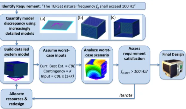
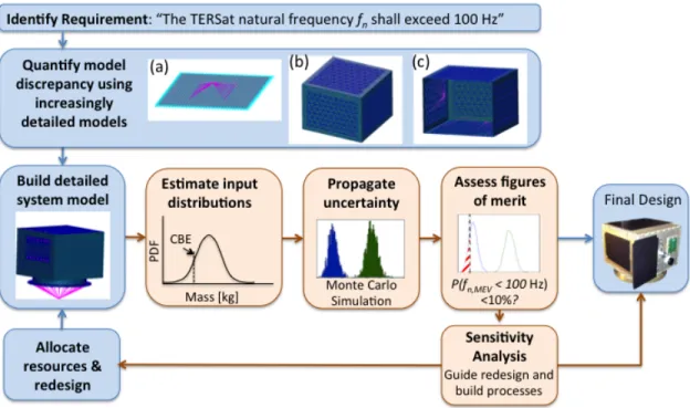
1-1 Traditional Spacecraft Design Approach . . . 19 1-2 Proposed Spacecraft Design Methodology includes uncertainty
prop-agation and sensitivity analysis to reduce the need for costly extra redesign steps late in program development . . . 21 1-3 Examples of exponential entropy for Gaussian, uniform, triangular,
and bimodal distributions . . . 24 1-4 Photograph of the TERSat prototype . . . 29 2-1 Setup of test system example . . . 32 2-2 Distribution of System TRLs after improving one part/subsystem by
one TRL based on two measures of uncertainty in the system showing that complexity was more effective for this test system . . . 35 2-3 Mass Probability Density Function with Improved TRLs selected based
on Mass Margin and Complexity . . . 36 2-4 Comparison of which approach caused the greatest improvement in
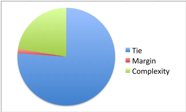
probability of meeting requirements, based on 1000 trials. Most of the results were ties, but of the remaining 10%, for 8% complexity was the superior guide for resource allocation . . . 37 2-5 Continuing timesteps with each approach until each reaches a
proba-bility under 10% . . . 38 2-6 Comparison of which approach caused the greatest improvement in
probability of meeting requirements using multiple TRL improvement steps, based on 1000 trials . . . 39
3-1 Illustration of TERSat with deployed 2.5m antenna booms . . . 42
3-2 Illustration of interaction between TERSat and DSX . . . 44
3-3 Overview of TERSat Prototype . . . 46
4-1 Histograms of mass budget Monte Carlo analysis over the course of the program . . . 57
4-2 Probability Density Functions of mass budget Monte Carlo simulation over the course of the program . . . 58
5-1 TERSat Structural Design Summary . . . 64
5-2 Finite Element Analysis Approach . . . 66
5-3 Finite Element Analysis model summary . . . 69
5-4 First mode of 101 Hz . . . 70
5-5 Stress analysis results of ESPA interface spacecraft panel . . . 71
5-6 Stress analysis results of the battery box . . . 72
5-7 Revised first mode of 109 Hz . . . 73
5-8 Histogram of Monte Carlo Analysis Results of CDR versus post-CDR 76 5-9 Probability Density Function of Monte Carlo analysis results of CDR versus post-CDR . . . 77
5-10 Histogram of Monte Carlo Analysis Results . . . 78
5-11 Probability Density Function of Monte Carlo analysis results . . . 79
5-12 Probability Density Function of Monte Carlo analysis results . . . 81
6-1 Photographs of the TERSat Prototype show the addition of smaller components . . . 86
6-2 TERSat STACER Shake Test Unit. The STACER was secured to the shake test interface plate with clamps to simulate the mounting of the STACER to the TERSat structure. A mesh cover protected surrounding workers from accidental deployment of the STACER. . . 89
6-3 TERSat STACER Shake Test Anomaly. The STACER antenna was not adequately secured with the TERSat housing design and shook loose during testing along the axis of the antenna. . . 91 6-4 The addition of a stopper to the TERSat STACER test setup prevented
the STACER from shaking loose during testing along the axis of the antenna. . . 92 6-5 TERSat STACER Shake Test, Final Configuration. The STACER
assembly successfully completed the rest of the shake test. . . 94 6-6 Comparison between TERSat subsystem mass predictions at PQR and
measured values of the as-built prototype. While there were substantial changes in subsystem masses, the sum of the changes was small (less than 2% of the CBE at PQR . . . 95
List of Tables
3.1 Mission Statements and Success Criteria . . . 45
3.2 TERSat Mass Budget . . . 47
3.3 TERSat Power Budget . . . 47
3.4 Payload Design Parameters . . . 48
4.1 Subsystem Mass Complexities after CDR . . . 59
5.1 Materials Data . . . 65
5.2 Modal Analysis Results, First Iteration . . . 70
5.3 Stress Analysis Results, First Iteration . . . 71
5.4 Modal Analysis Results, First Iteration . . . 72
5.5 Modal Analysis Results, First Iteration . . . 73
5.6 Density Inputs to Finite Element Analysis . . . 75
Chapter 1
Introduction
Space programs are increasingly complex and suffer from uncertainty in many quan-tities of interest, leading to schedule and cost overruns. NASA’s “Faster, Better, Cheaper” approach worked for some programs (for example, Stardust as described in Atkins, 2003 [3]), but for several high-profile Mars missions this approach led to failure and the aerospace industry abandoned it [17]. While many papers have been written giving statistics of cost and schedule overruns in aerospace systems, we can build on this literature by identifying practical next steps in implementing the knowledge from these statistics to efficiently manage uncertainty in space systems. As summarized by Collopy (2011), leading industry systems engineers agreed during a series of NASA and NSF workshops that uncertainty management is one of the most needed areas of research in space systems engineering [8]. According to Collopy, “Systems engineerings first line of defense against uncertainty is a semi-quantitative risk management process with no rigorous foundation in the theory or calculus of probability.” [8]
We propose a methodology for spacecraft design which consists of starting with traditional system models and using these models to characterize uncertainty in model outputs with Monte Carlo simulation, sensitivity analysis, and complexity character-ization to reduce the need for expensive redesign. We use the Trapped Energetic Radiation Satellite (TERSat) as a test case for evaluating this methodology.
quanti-ties of interest. We use uncertainty analysis of mass budgets to show how to integrate the statistics of space program mass budgets with space program development. Next, the methodology is extended to more complex analysis with finite element analysis of TERSat. Finally, the TERSat lessons learned are documented to reflect on the results of program uncertainty.
1.1
Motivations for Incorporating Space Program
Uncertainty Statistics
Space programs are complex systems and suffer from large uncertainties in cost and schedule. For example, a NASA study found that to obtain better than 65% joint con-fidence level in cost and schedule, programs need to maintain 30-50% reserve in cost budgets and schedules[23]. Such high reserves are considered politically untenable[23]. Critical quantities of interest in a program include cost, schedule, and mass margin, and these are often closely coupled. According to Karpati et al. (2012),
Especially for satellite systems, the mass margin is intimately tied to other engineering and management goals such as performance, cost, schedule, and risk. As the mass of the object to be launched approaches the throw-mass limit of the launch vehicle, decisions by the development team skew more aggressively toward mass savings at the expense of some combina-tion of performance, cost, schedule, or risk. Not all satellite development programs that are over their mass controls are cancelled, but the converse is usually true...that is, cancelled programs are almost always over their mass controls. [20]
The reason changes in certain quantities of interest can have such a great effect is that changes in any part of a system can propagate through a system. Giffin and de Weck (2009) studied the propagation of changes in complex systems and found that changes in components at the intersection of major functional areas have the greatest
Figure 1-1: Traditional Spacecraft Design Approach
effects, but even changes in one subsystem can still affect subsystems that are not closely related on a Design Structure Matrix (DSM) [11].
Many papers have studied the historical trends of these quantities of interest in space system development. For example, Kipp presented statistics of mass, power, schedule, and cost of numerous NASA missions [21]. In this paper, Kipp et al. correlated growth in these quantities of interest with instrument type, mass, and power. Another example of statistical studies of space programs is Dubos et al. (2007), which compared technical readiness level of space systems with trends in program schedule [14]. Finally, Browning (1999) identified sources of schedule risk in complex system development [7].
These studies showed that space systems tended to increase in mass, cost, and schedule over time and they help to identify the drivers for these difficulties. How-ever, a next step is needed to bridge the gap from the results of these papers to
implementing the knowledge in a real space system. This thesis proposes methods for incorporating uncertainty statistics in mass, natural frequency, and schedule into complex spaceflight program development.
For systems where a system of equations can fully describe the system, optimiza-tion under uncertainty is possible. For complex space systems, currently there is a limit to how much of the system can be described only by a system of equations with-out some human understanding in the loop. By incorporating studies of uncertainty with software tools currently in use, greater insights can be gained while maintaining practicality.
1.2
Research Objectives and Methodology
The objective of this work is to develop a spacecraft design methodology that reduces cost and schedule overruns while meeting program design requirements by identifying issues and design drivers early in development using uncertainty and sensitivity anal-ysis of detailed system models. The Trapped Energetic Radiation (TERSat) program is used as a test case for evaluating this methodology.
The research approach was to define the methodology and then apply it to TER-Sat as a test case. We evaluate success based on both quantitative and qualitative measures:
• Quantitative: Demonstrate reduction in risk of failing a requirement
• Qualitative: Guide for layout fine-tuning, improved understanding of uncertain-ties
As illustrated in Figure 1-2, the methodology begins with requirements on quan-tities of interest in the system. Validated models of increasing fidelity are built to model the quantity of interest. Then, rather than making assumptions about what the worst-case scenario might be, probability distributions are determined from his-torical data for inputs to the models. These uncertainties are propagated in the model using Monte Carlo simulation to determine the uncertainties in the output.
Figure 1-2: Proposed Spacecraft Design Methodology includes uncertainty propaga-tion and sensitivity analysis to reduce the need for costly extra redesign steps late in program development
The figure of merit of this methodology is the probability of failing the require-ment. Sensitivity analysis and measures of complexity can then be used to refine requirements on related quantities of interest or help in redesigning the system.
The first quantity of interest under study was the TERSat mass budget. This was selected for two reasons: (1) mass is a critical quantity to monitor because TERSat had a requirement to stay under 50 kg and (2) mass budgets are simple types of models because the numbers in the models sum linearly.
The next quantity of interest under study was the TERSat first fundamental frequency. TERSat has a requirement that the first mode must exceed 100 Hz. Finite element models using traditional margin techniques produced an expected value of 101 Hz for the baseline design, but this approach does not produce error bars on the result. Following the above methodology, the uncertainties identified in the mass budget analysis were used as inputs for the spacecraft modal analysis to show how likely it was that the satellite would meet requirements. Because the uncertainty analysis of the mass budget showed significantly higher likelihood of meeting the mass requirement than the frequency uncertainty analysis showed of meeting the frequency requirement, mass was added to stiffen the structure.
1.3
Literature Review
The literature review is focused on three areas: system complexity, system tainty, and current practices in space systems for managing complexity and uncer-tainty.
1.3.1
Measures of Complexity in Complex System Design
and Implementation
According to Shalizi (2006), “a complex system, roughly speaking, is one with many parts, whose behaviors are both highly variable and strongly dependent on the be-havior of the other parts.” [30] However, there are many methods of defining system
complexity. In a website, Shalizi even humorously summarizes the various complexity metrics by saying “Every few months seems to produce another paper proposing yet another measure of complexity, generally a quantity which can’t be computed for any-thing you’d actually care to know about, if at all. These quantities are almost never related to any other variable, so they form no part of any theory telling us when or how things get complex, and are usually just quantification for quantification’s own sweet sake.” [31]
In general, system complexity definitions fall into two categories, structural and behavioral. Structural complexity is a measure of how complex the architecture of a system is, while behavioral complexity is a measure of how unpredictable the behavior of a system is. Here we survey some of each type of metric. The exponential entropy metric was selected for use in the methodology we present.
Behavioral Complexity Metrics
Behavioral complexity draws from information theory. There are several definitions. Kolmogorov defined complexity based on the amount of entropy in a string [22]. Arthur Ferdinand defined complexity as a measurement of the errors in a system, in which a perfectly simple system has 0 complexity and no errors [2]. The META exponential entropy complexity metric from Willcox et al. (2011) is derived from the concept of differential entropy from information theory [39]. Differential entropy is defined as:
h(X) = − Z
Ωx
fx(x) log(fx(x))dx (1.1)
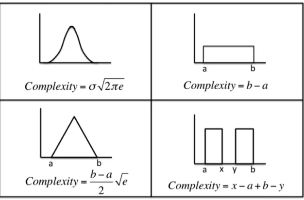
For example, for a uniform distribution spanning a to b, the differential entropy is ln(b − a). The exponential entropy metric defines complexity as:
C(Q) = eh(Q) (1.2) Thus, the units of the exponential entropy metric are the same as the units of the quantity of interest. This makes the exponential entropy metric more intuitive.
Figure 1-3: Examples of exponential entropy for Gaussian, uniform, triangular, and bimodal distributions
For example, for a uniform distribution, the exponential entropy is simply b-a. Some examples of distributions and their complexities are shown in 1-3.
Structural Complexity Metrics
de Weck and Murray (2011) [25] present an example of structural complexity that uses a combination of complexity terms. In this work, complexity is composed of three parts: structural, dynamic, and behavioral. These three terms are multiplied together to achieve an overall system complexity.
The structural complexity term is based on graph theory, in which the components of the system are nodes and component interfaces are edges of the graph. This definition is derived from the measure of energy of molecules.
The dynamic complexity is related to Shannon entropy, similar to the exponential entropy metric, but in this case dynamic complexity measures the interdependence of different quantities of interest in the system.
Another definition of complexity, specifically developed for space systems, is the Bearden (2003) model which relies on twenty one factors including design life, max distance from Earth orbit, ADCS type, and number of payload instruments. This complexity metric is used to determine the risk of pursuing an interplanetary mission since these have constrained schedules [4].
Complexity Metric Selection
Each of these measures of complexity is useful for different applications. For under-standing uncertainty, behavioral complexity is the most relevant complexity metric. The exponential entropy complexity metric offers a measure of complexity with con-venient units and useful response to discrete alternatives. This definition provides a complement to standard deviation as a measure of uncertainty and was selected for this methodology.
1.3.2
Uncertainty of Quantities of Interest in Complex
Sys-tem Design and Implementation
According to [5], there are three categories of uncertainty:
• Aleatory Uncertainty: This type of uncertainty represents the random errors in a system. On a target, this type of uncertainty represents the distribution, or precision, of the hits.
• Epistemic Uncertainty: This type of uncertainty represents systematic uncer-tainty in a system. In the example of a target, this represents the accuracy of the hits.
• Ambiguity: This represents a lack of system knowledge and behaves similarly to epistemic uncertainty.
Part of the META approach to systems engineering is that system uncertainty should be quantified and tracked throughout the systems engineering process. Un-der the META approach, both aleatory and epistemic uncertainty are combined into probability density functions. Sondecker (2011) went as far as describing how to iden-tify quantities of interest to use in the META framework, but did not implement the META complexity evaluation [33]. We take the next step by performing uncertainty analysis on spacecraft quantities of interest.
1.3.3
Notes on Optimization
Optimization is related to the topic of uncertainty analysis of complex systems. Some optimization problems deal with uncertainty of complex system design. Robust opti-mization and stochastic optiopti-mization are related to this field.
Stochastic optimization uses random variables to represent inputs in the setup of optimization problems. The goal of stochastic optimization is to find a good result with uncertain inputs using efficient computing. Similarly, robust optimization attempts to find an optimal solution that is optimal for a range of inputs. In contrast, deterministic methods fully sample a space, but this is inefficient for complex systems. In complex system design, optimization is often not the correct problem descrip-tion. In most cases, space systems need to achieve certain requirements such as mass, but it is not necessary to reach an absolute minimum mass to be successful. Thus, simply characterizing the uncertainty through Monte Carlo analysis and using sen-sitivity analysis to help determine resource allocation may be sufficient to address design issues without optimization.
However, these methods are not commonly used for complex multidisciplinary sys-tems such as space system design because these methods require a problem structure that is not widely found in these systems. Therefore we did not apply optimization to this methodology.
1.3.4
Current Practices in Complex Space System
Uncer-tainty Management
The most typical way uncertainty is accounted for in systems engineering is through margin and contingency. Karpati et al. (2012) provides an excellent summary of margin and contingency in space systems and provides guidelines for treatment of each by subsystem. There are also standards for accounting for margin. For example, the leading standard for mass margins is AIAA S-120-2006. Margins are difficult to account for because both under and over allotment of margin can lead to problems in program development. According to Karpati et al. (2012)
If a project takes on overly conservative margins at the beginning of a program, they may have let some mission performance go unrealized, or put themselves in an early decision to use expensive lightweight materials or risky lightweight technology. But projects that take margins that are too low walk the path of many developments where margins erode before launch and even more costly (or risky) late design trades must be made. [20]
However, this traditional method of margin management is limited in capability. It treats all uncertainties as a uniform probability distribution and does not account for the more detailed statistical results of studies like Browning’s. Emmons approaches this problem and provides helpful general strategies for reducing cost and schedule overruns, such as developing instruments before developing the spacecraft to avoid costs of “marching armies” when instruments are delayed [15].
Some new approaches in systems engineering allow space systems engineers to make architecture decisions with uncertainty in mind. Silver and de Weck (2007) developed “Time-Expanded Decision Networks” which allow a systems engineer to select more flexible architectures to account for uncertainties in the system [32].
de Weck’s 2006 paper on Isoperformance is another example of designing under uncertainty. In this paper, de Weck showed that optimization problems can return not just a single optimal point but a family of performance-invariant points that
can be compared by cost or other criteria [13]. Some people treat system design as an optimization problem, as Croisard (2010) did when using Evidence theory in optimizing the wet mass of the BepiColombo mission [10]. Wertz treats uncertainty in a system as a risk that can be traded with productivity. Wertz uses Markov chains to represent the chain of events of experiments, and simulates the performance loss with each ordering of experiments based on the risks of each experiment [38].
The most widespread new technique for uncertainty management in aerospace is the Joint Confidence Level technique used at NASA. This approach requires programs to demonstrate 30-50% reserves in cost and schedule. This has spurred some research in how to use Monte Carlo analysis for characterizing uncertainty in cost and schedule, such as Cornelius (2012) [9]. This technique can be extended to other quantities of interest, as we demonstrate in this thesis.
1.4
TERSat Program Summary
The Trapped Energetic Radiation Satellite (TERSat) is a 32 kg student-built nanosatel-lite developed under the University Nanosatelnanosatel-lite Program (UNP). The TERSat pro-gram began in the fall of 2010 and a prototype was completed in January of 2013. The TERSat program will investigate how VLF waves interact with the radiation en-vironment in Low Earth Orbit (LEO) by deploying a 5 m dipole, using a transmitter to radiate VLF waves over a range of voltage levels up to at least 600 V, frequencies from 350 kHz, and a range of magnetic field orientations. TERSat will also measure the strengths of the echoes with a low noise VLF receiver. A photograph of the TERSat prototype is shown in Figure 6-1.
Performing these experiments will help determine how well a deployed antenna system can overcome the antenna sheath impedance to radiate at VLF frequencies in the LEO plasma environment, how efficiently can VLF energy be radiated at LEO altitudes, and if we can explain the up to 1000 times (20 dB) model vs. observational differences in Starks et al. (2008). These experiments will be critical to the success of future missions to use VLF emissions for radiation belt remediation. The TERSat
Figure 1-4: Photograph of the TERSat prototype
experiments will also allow scientists to better calibrate underlying plasma physics models which have orders of magnitude uncertainties for geometries at LEO altitudes. TERSat’s requirements derive from the UNP requirements and from the two mis-sion statements:
MS1 Demonstrate and characterize transmission of low frequency (VLF) waves in the inner Van Allen radiation belt over a range of frequencies, over a range of power levels, and over a range of orientation to the magnetic field.
MS2 Demonstrate the ability to receive echoes/reflected signals resulting from the transmitted pulses using an on-board VLF receiver.
There are many technical performance measures that are derived from these re-quirements, including mass, power, and natural frequency. We focus on mass and natural frequency as the quantities of interest in the TERSat structural design test case for evaluating our proposed methodology.
Chapter 2
Methodology
This chapter describes in greater detail the methodology for characterizing uncer-tainty and complexity of quantities of interest. The methodology follows a bottom-up approach, first studying the uncertainties of individual inputs to models of quantities of interest. Next, these are incorporated into a model of the quantity of interest. For example, the model of the natural frequency of a spacecraft would be the finite element model of the spacecraft. Lastly, Monte Carlo simulation and sensitivity anal-ysis show the relative importance of different parameters to complex models. A test system is described in this chapter to illustrate the methodology.
2.1
Test System Setup
To illustrate this methodology, a test system can be used as a simple, generic exam-ple of a system. A single quantity of interest, in this case system mass, has inherent uncertainties due to uncertainties in the masses of the subsystems. Typically, if un-certainty is even considered, items with larger mass growth allowance are targeted for uncertainty reduction resources. The proposed methodology employs the exponential entropy metric instead.
In the most basic test system setup, resources are allocated to increase the tech-nical readiness level (TRL) of a subsystem by one. In one case, the subsystem with
Figure 2-1: Setup of test system example
the largest mass margin is targeted, while in the other case the subsystem with the largest complexity is targeted. This is illustrated in Figure 2-1.
To set up the problem, the system is assigned some parameters: number of parts/subsystems, distribution of TRL, and order of magnitude of mass. Then a list of subsystems are generated based on these parameters. Each subsystem has a TRL (randomly assigned using the program TRL distribution shape and with for the random number generation), a mass (randomly generated within 50% of the mass order of magnitude value), and a margin, which is determined by the TRL the sub-system has been assigned. This allows a variation in subsub-systems with each run of the analysis, enabling Monte Carlo analysis.
Next, the subsystem masses are compiled into mass probability density functions. To do this, many masses for each subsystem are generated using the mass margin to bound the uncertainty of the subsystem. In this illustrative example, subsystems with
higher TRLs use triangular distributions to account for engineers’ greater certainty in the subsystem design, while subsystems with lower TRLs have uniform probability density functions. (For reference, the actual mass budget simulation chapter uses different PDFs based on actual historical data).
These lists of subsystem masses are then compiled into histograms. Kernel Density Estimation (KDE) allows these to be turned into probability density functions, which are then used to compute complexity. To perform the KDE, the built-in KDE function in the Python SciPy package is used. This method assumes gaussian distributions for the kernels and uses the Scott rule of thumb method for determining the bandwidth of the distributions. According to Zucchini (2003), the shape of the kernel distribution does not have a significant effect on the KDE output [40]. The Scott rule of thumb is commonly used in cases of less than five dimensions, which this is [29].
These PDFs from the KDE are binned and each bin and probability density are integrated to find the complexity per Equation 1.2.
Now the system has both margin and complexity for each subsystem. Subsystems with larger margins and complexities are more uncertain that subsystems with lower margins and complexities. In the automated test system, the subsystem with the higher margin and complexity are selected for improving the subsystem TRL. Perfor-mance of each is then estimated by assuming a reference value for a requirement and determining the improvement in probability of meeting the requirement using each technique.
This test system has limitations. By automating every step, the intuition of the system engineer is removed. Interactions between subsystems are known to the systems engineer but automatically tracking and updating these interactions and their related uncertainties is outside the scope of this thesis. In a real program, which will be illustrated in later chapters, the systems engineer would use the complexity information to inform decision making in combination with the other information the system engineer has. Additionally, in a real world setup, TRL improvements can happen in parallel.
improve a subsystem by one TRL are equal, regardless of subsystem or initial TRL. Presumably this is not the case, as transitions between some TRL numbers require building of simple prototypes, while other transitions require significant field testing.
2.2
Test System: One Timestep Example
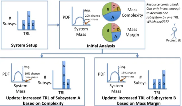
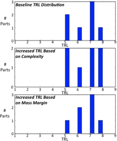
The first test system demonstration is of taking one TRL improvement step. The test system code randomly generates a TRL distribution for a system based on in-puts regarding likelihood of each subsystem TRL. Figure 2-2 shows an initial TRL distribution and the TRL distributions following the differing TRL improvement steps recommended by the mass margin uncertainty and complexity methods. Here, the complexity approach recommended improving one of the TRL 7 subsystems to TRL 8, while the mass margin approach recommended improving a TRL 5 subsystem.
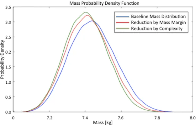
The mass probability density functions of these TRL distributions are shown in Figure 2-3. While both mass margin and complexity approaches reduced the system mass uncertainty, the complexity approach was slightly more effective for this case in shifting the system mass curve to the left and reducing the standard deviation of the curve.
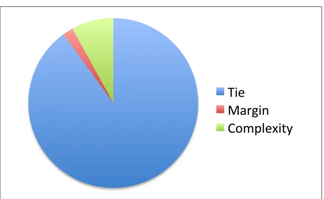
While in this example, complexity and margin approaches recommend different subsystems for TRL improvement, in many runs the two approaches recommend the same subsystem. As shown in Figure 2-4, a study of 1000 runs with these baseline inputs found that approximately 90% of the time complexity and margin recommend the same subsystem for TRL improvement. 8% of the time Complexity recommended a better course of action for TRL improvement than did Margin, measured by which subsystem TRL change caused greater improvement in probability of meeting the system mass requirement.
This is as expected. Complexity accounts for the shape of the distribution chang-ing as the subsystem uncertainty decreases with increaschang-ing TRL, while margin only accounts for the width of the distribution.
Figure 2-2: Distribution of System TRLs after improving one part/subsystem by one TRL based on two measures of uncertainty in the system showing that complexity was more effective for this test system
Figure 2-3: Mass Probability Density Function with Improved TRLs selected based on Mass Margin and Complexity
Tie
Margin
Complexity
Figure 2-4: Comparison of which approach caused the greatest improvement in prob-ability of meeting requirements, based on 1000 trials. Most of the results were ties, but of the remaining 10%, for 8% complexity was the superior guide for resource allocation
Figure 2-5: Continuing timesteps with each approach until each reaches a probability under 10%
2.3
Test System: Continuing Timesteps Example
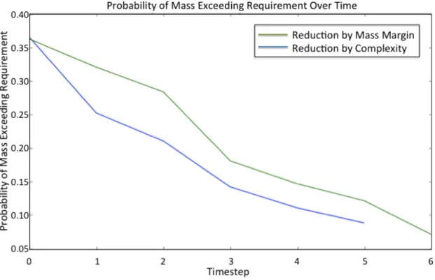
To further illustrate this point, the test system can also be run for many timesteps to see which approach reduces uncertainty most effectively with the least resources. Figure 2-5 shows an example. In this case, complexity proved to be a more effective approach to reducing uncertainty in the test system’s mass distribution than mass margin. While both approaches reduced the probability of failing the mass require-ment, the complexity approach was able to reduce the probability to under 10% with fewer steps than the mass margin approach required. In the real world, this would translate to fewer resources being required to reduce system risk.
In this example, the complexity approach is more effective than mass margin at reducing uncertainty in the system. However, in many cases the two approaches show roughly the same rate of improvement.
Tie
Margin
Complexity
Figure 2-6: Comparison of which approach caused the greatest improvement in proba-bility of meeting requirements using multiple TRL improvement steps, based on 1000 trials
Figure 2-6 shows that 76% of the trials resulted in a tie, with both approaches requiring the same number of steps to reach 10% probability of failing requirements. In 23% of the trials, complexity required fewer steps than margin to reduce the probability of failure to within 10%, and in only 1.4% of trials margin produced the better course of action.
These results show that most of the time, either approach will work, when the two differ complexity gives the better result. Of course, this hinges on inputs. A sensitivity analysis is required to determine what factors influence these percentages.
2.4
Test System: Parameter Variation
There are several factors that this analysis is sensitive to.
• Shape of distributions based on TRL: The analysis is based on assumptions about how the shape of the subsystem-level probabilities change with
improve-ments in TRL, but knowledge of the shape of these distributions is poor. • Distributions of subsystem TRL for the current baseline: Could the utility of
the tool vary with how developed the system is?
• Relative subsystem mass properties: The mass properties currently only vary by +/- 25%, but a wider distribution could skew results universally towards the heavier system.
• Stage in design (whether or not discrete architecture trades are open): Mass margin is not well defined for subsystems with open architecture trades, while this can be simply represented by a multimodal distribution in complexity anal-ysis. Various mass margin approaches will be compared with the complexity analysis results.
The test system example could be carried out to investigate each of these. How-ever, the simple example is only used to demonstrate the methodology, so we will proceed to answer these questions with the TERSat case study.
Chapter 3
Overview of the TERSat Program
Radiation damage caused by interactions with high-energy particles in the Van Allen Radiation Belts is a leading cause of component failures for satellites in low and medium Earth orbits (LEO, MEO). Strong solar storms can cause significant increases in radiation levels in the Van Allen belts leading to severe damage to nearby satellites and a significant reduction in satellite life expectancy. Solar storms and coronal mass ejections can also cripple or permanently disable spacecraft. Shielding against such events can increase the cost of space mission due to the additional mass and is not always even effective. However, it has been suggested that emissions of Very Low Frequency (VLF) waves could dissipate electrons from the radiation and mitigate the bulk of satellite exposure to intense radiation events [26].
Very Low Frequency (VLF) electromagnetic waves have been shown to couple en-ergy to high-enen-ergy radiation belt electrons and change their properties. VLF waves from lightning and plasma hiss from magnetospheric reconnection can scatter the pitch angle of high-energy particles, such that they rejoin the neutral lower atmo-sphere [18]. Due to the ionospheric plasma cutoff frequency limiting the efficiency in coupling VLF from the ground to space, it has been proposed that space-based antennas transmitting VLF waves could similarly help reduce the effects of radiation by scattering electrons.
However, the interaction between a VLF transmitter and the plasma environment is not sufficiently well understood. For example, Starks et al. (2008) summarizes how
Figure 3-1: Illustration of TERSat with deployed 2.5m antenna booms
models of field strength in the plasmasphere away from the magnetic equator appear to be overestimated by a large amount, 10-20 dB, and underestimated by 15 dB at the magnetic equator for L less than 1.5. The implication is that there are important physics not understood or captured in the ionosphere and LEO altitudes [34].
It is clear that on-orbit experimentation and demonstration are needed to analyze how best to tune and couple VLF energy to the electrons and ions even though terrestrial VLF equipment is well understood and low-risk.
The Trapped Energetic Radiation Satellite (TERSat) is a 32 kg student-built nanosatellite that will analyze how VLF waves interact with the radiation environ-ment at 550 km altitude by deploying two 2.5 m antennas to form a 5 m dipole, using a transmitter to radiate VLF waves over a range of voltage levels up to at least 600 V, frequencies from 350 kHz, and a range of magnetic field orientations. TERSat will also measure the strengths of the echoes with a low noise VLF receiver.
The TERSat science mission complements that of AFRLs Demonstration and Science Experiments (DSX) satellite. TERSat will perform a subset of the DSX experiments at a much lower orbit, giving insight into the effects of altitude-dependent plasma density and magnetic field strength on the wave-particle interactions. TERSat is also capable of interacting with DSX for bistatic experiments if the mission periods overlap. A CAD image of TERSat is shown in Figure 3-1.
and potentially reduce Van Allen Belt radiation by improving our understanding of transmitting and receiving VLF waves in a LEO satellite plasma environment.
3.1
Mission Overview
The Trapped Energetic Radiation Satellite (TERSat) is a student-designed nanosatel-lite (5 50 kg) that will investigate the ability of space-based Very Low Frequency (VLF) radio transmission to reduce the population of harmful high-energy particles in the inner Van Allen radiation belts. TERSat was conceived and first developed as MITs entry into the AFRL University Nanosatellite Program (UNP) competition and received design and engineering model support from UNP and NASA JPL. To date, TERSat has completed UNP-7s preliminary design review (PDR), critical de-sign review (CDR), the pre-prototype build Proto-Qualification Review (PQR), and the flight competition review (FCR). On June 30, 2012, TERSat flew a prototype VLF transmitter and tested their ground station receiver as a participant in AFRLs Student Hands On Training (SHOT II) high altitude balloon experiment.
TERSat will radiate VLF waves and measure the strength of the echoes. TERSat could also receive echoes from DSX transmissions, and could transmit for detection by the DSX receiver. The bus and deployed antennas are illustrated in Figure 3-1. TERSats baseline orbital altitude is 550 km, but altitudes up to 600 km will still satisfy the UNP de-orbit requirement and are thus acceptable.
Experiment parameters: TERSat will radiate VLF waves at 3, 25, and 47 kHz, 100, 300, and 600 V, and orientations of perpendicular, 45 degrees, and parallel to the magnetic field lines. TERSat will start with lower voltages and step up to at least 600 V due to uncertainty in the voltage at which arcing begins to occur.
A possible addition to the experiment plan would be to interact with the AFRL satellite DSX. Such an interaction would add an additional dimension to the wave-particle interaction measurements. According to Bortnik (2002), VLF waves not only travel and reflect along one magnetic field line, they also travel radially around and along other magnetic field lines [6]. This would allow TERSat and DSX to monitor
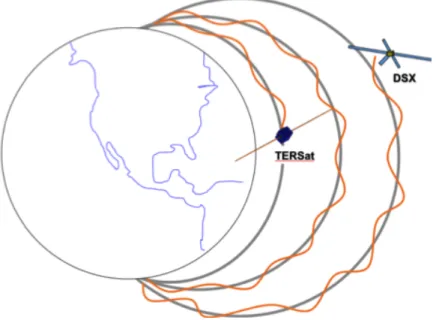
Figure 3-2: Illustration of interaction between TERSat and DSX
each others transmissions and provide a better understanding of radial VLF wave propagation. This interaction is illustrated in Figure 3-2. The orange curve indicates the VLF waves motion along the magnetic field lines. As noted by Bortnik (2002), the ability of a VLF wave to move radially has a dependence on transmitted frequency [6].
Additionally, because plasma density and magnetic field strength varies with or-bital parameters and altitude, TERSat could repeat DSX experiments to provide an understanding of how the density and field strength variations affect VLF propaga-tion.
3.2
Requirements and Success Criteria
The TERSat Mission Statements are shown in Table 3.1. To be successful, TERSat must accomplish both of the minimum success criteria: (i) transmit and characterize how effectively a VLF pulse is launched perpendicular to the local magnetic field, and (ii) receive VLF signals using an on-board receiver.
The objective success criteria characterize the effects of frequency, voltage (power) and magnetic field orientation on how well VLF waves interact with electrons in
Table 3.1: Mission Statements and Success Criteria Statement Description
MS1 Objective Success Criteria: Demonstrate and characterize transmis-sion of low frequency (VLF) waves in the inner Van Allen radiation belt over a range of frequencies, over a range of voltages, and over a range of orientations to the magnetic field.
Minimum Success Criteria: Demonstrate and characterize trans-mission of low frequency (VLF) waves in the inner Van Allen radi-ation belt near 50 kHz, at one voltage, with an orientradi-ation perpen-dicular to the magnetic field.
MS2 Objective Success Criteria: Demonstrate the ability to receive echoes/reflected signals resulting from transmitted pulses using an on-board VLF receiver.
Minimum Success Criteria: Demonstrate the ability to receive VLF signals using an on-board VLF receiver.
plasma. The minimum success criteria address a more basic but still critical science question: can a deployed antenna system overcome the antenna sheath impedance to radiate at VLF frequencies in the LEO plasma environment? Self-monitoring of the relative phase between the voltage and current on the transmitter should provide insight as to whether effective transmission occurs (if the voltage and current are in-phase, the system is well-matched). It is important to demonstrate the independent functionality of the VLF receiver by measuring other (natural or man-made) VLF signals in addition to any received self-echoes. For example, this would be useful if a reasonable match is measured at the transmitter and yet no self-echo is received.
3.3
Design Overview
TERSat is a 41 x 41 x 30 cm satellite with an as-built prototype mass of 32 kg. The TERSat payload will deploy two 2.5 m STACER antennas, transmit VLF waves using a student-designed and fabricated transmitter, and measure the strengths of the echoes and other VLF signals with a Stanford VLF receiver identical to the DSX receiver. The solar panels consist of donated solar panels from Vanguard and are body-mounted on five of the six outer structural panels. All electrical components are
Figure 3-3: Overview of TERSat Prototype
contained within the aluminum 6061-T6 chassis, including the batteries, computer, communications, and power electronics. The Attitude Determination and Control System (ADCS) uses three reaction wheels in conjunction with three customized torque coils. The spacecraft walls consist of skinned isogrid Al6061-T6 panels. Place-ment of these components is shown in Figure 3-3.
TERSat bus electronics take advantage of CubeSat technology, including a Pump-kin Motherboard and processor, a Clyde Space EPS, and an MHX S-band commu-nication system. This enables standardization of interfaces and reduced wiring needs for rapid design and integration. It also reduces the qualification testing associated with custom parts.
3.4
Technical Performance Measures
The TERSat Program has tracked technical performance measures including mass, power, data, and communications budgets to ensure design success. A master equip-ment list (MEL) has also been used to keep track of all system components.
As shown in the PQR mass budget in Table 3.2, the structures subsystem dom-inates the mass of TERSat. To ensure structural stability under earlier high uncer-tainty of other subsystems, the structure was over designed. The panels are formed of
isogrid aluminum rather than a more weight-efficient composite-honeycomb sandwich design to reduce complexity.
Table 3.2: TERSat Mass Budget
Subsystem Subtotal [kg] Margin Mass Budgeted [kg] Structures/Thermal 14.6 15% 16.8 Avionics/Comm. 3.03 15% 3.5 ADCS 1.00 15% 1.15 Power 6.72 25% 8.40 Wiring 3.00 50% 4.5 Payload 4.88 25% 6.10
System Subtotal 33.2 System Total 40.4
The TERSat power budget is shown in Table 3.3. In most modes, the thermal subsystem dominates TERSat power usage. Heaters protect temperature-sensitive components such as batteries when the rest of TERSat does not produce enough power to compensate in heat production.
Table 3.3: TERSat Power Budget
Subsystem Commissioning Nominal Payload Tx Safe Mode Comm 4.6 W 0.9 W 0.3 W 4.6 W Avionics 2.5 W 2.5 W 2.5 W 2.5 W ADCS 2.8 W 3.5 W 4.0 W 0.4 W Thermal 7.5 W 7.5 W 0.0 W 7.5 W Power 2.1 W 1.7 W 1.5 W 0.9 W Payload 0.2 W 0.0 W 40 W 0.0 W Total 19.9 W 16.2 W 48.2 W 16.0 W
One interesting feature of the power budget is the payload power during operation. While transmitter power can be estimated based on the plasma interaction models, only the input voltage (100-600 V) can be known with certainty as the radiated power depends on how well the transmitter circuit is tuned to the plasma environment, which cannot be known or adjusted until experiments commence on-orbit. Measurement and characterization of the power drawn is one of the expected results of the experiment.
3.5
Payload Design
The TERSat payload consists of three key elements: the STACER antennas, the VLF transmitter electronics, and the Stanford Wave-induced Precipitation of Electron Radiation (WIPER) VLF receiver. The transmitter electronics and the receiver each have a dedicated chassis, and although electrically connected, the STACER antennas mount to opposite panels to create a dipole when deployed. The payload design parameters were selected using a Matlab simulation of electromagnetic radiation in a plasma. The simulation predicts the expected power output for a range of inductance values assuming a 600 V input. As the inductance values were tuned from 0.3 H up to 1 H, the power output and resonant frequency of the circuit varied.
The final design parameters are shown in Table 3.4. The antenna length of 5 m was found to be sufficient for experimental needs while still short enough to be easily accommodated by existing facilities when deployed for testing. A peak voltage of 600 V is expected to provide sufficient margin on the minimum voltage of arcing in plasma.
Table 3.4: Payload Design Parameters Parameter Value
Antenna Length 5 m Peak Voltage in 600 V Frequency Range 3-50kHz Inductance Range 0.2-3.0 H
For the antenna, the STACER system developed by Ametek Hunter Spring was selected. The STACER is a coiled spring-type mechanism. For lengths less than 10 m (35 ft) the STACER can be purchased as a pop-up one-time deployment model using stored elastic energy to fully deploy. The key benefits of the STACER system are its versatility and 600 mission flight heritage. The TERSat STACER will use a conductive Beryllium-Copper alloy as it provides both structural rigidity as well as the electrical conductance needed for the science mission. TERSat has purchased a STACER and designed and machined STACER deployment structures for
develop-ment. Testing is now underway, including deployment reliability, control dynamics, and interface testing.
During payload operation, the TERSat transmitter will radiate VLF waves for 1 to 30 seconds within the range of 350 kHz. At least 600 V will be supplied from the transmitter to the antenna in order to radiate these waves. The core of the transmitter is the H-bridge circuitry, which takes power from the battery pack and a low-voltage logic signal from a microcontroller. The H-bridge will trigger off of the microcontroller pulse and continuously switch the direction of the current supplied by the batteries and form a full square wave. The output voltage will then be fed into a transformer that will be used to step up the output voltage to the desired maximum of 600 V. This stepped-up voltage will be supplied to the payload in the form of a sinusoidal waveform (using an RLC circuit to tune/impedance match, which will also filter out high-frequency components of the square wave) and will be used to radiate VLF waves. The transmitter voltage and current will be measured and their phase tracked in order to provide power estimates as well as information on the impedance match. It is important to characterize the impedance of all components in the transmitter as a function of frequency during testing. Preliminary tests of an engineering model have shown that at a low voltage and frequency, the H-bridge and transformer will be able to generate high-voltage VLF sinusoidal output.
The TERSat VLF receiver uses the Stanford WIPER VLF receiver chip. This chip has a wide bandwidth and is capable of receiving from 100 Hz to 1 MHz [24]. It is also low power, requiring less than 0.5 W to operate. This chip will be placed on a PCB with supporting electronics. EMI filtering will maintain the sensitivity of the chip and scrub the incoming signal from the dipole antenna. The receiver chip will interpret the signal and the primary avionics computer will process the data. The WIPER chip and supporting electronics will be housed in an aluminum chassis mounted to a side panel of the spacecraft.
3.6
Program Schedule
Moving forward from the AFRL UNP-7 schedule through January 2013, TERSat will transition from a heavily focused design and engineering model phase to a flight build phase. Preliminary steps for this phase have already occurred through the development of FlatSat demonstrations. During the process of ETU assembly for the UNP PQR (proto-qualification review) and FCR (flight competition review), both component and integrated functionality tests were performed on the components to assess operation and durability of the satellite. Component testing will evaluate the operation of individual components. Integrated testing will analyze the interactions between subsystems by testing communication among components, verifying correct power levels are being supplied to the subsystems and payload.
Chapter 4
Mass Budget Analysis
Spacecraft mass is a source of cost increase. Increased mass reduces margins on structural design, and this can lead to costly redesign. Additionally, mass tends to increase over the course of a program in an unpredictable way. The current approach of standard mass margins often fails to adequately predict how much the mass of a system can grow [16]. In an Aerospace Corporation study, the average mass growth of 10 systems was 43% over the course of a program, while typical industry guidelines recommend 30% reserves (both relative to Current Best Estimate, or CBE) [16]. However, increasing the reserved margin is not necessarily the answer, as designing structures and mechanisms to uniformly accomodate possible heavier systems may be unnecessarily difficult and costly.
System mass growth has several common sources, categorized as internal or ex-ternal sources, according to the AIAA [35]. The inex-ternal sources of mass growth are:
• Better definition of the design (Internal) • Out of scope (External)
• Redesign (Internal/External)
• Maturing component design (Internal) • Error in previous estimate (Internal)
• Uncontrolled vendor changes (External) • Mass reduction activity (Internal) • Measured vs. calculated (Internal)
• Mass added for cost/schedule reduction (Internal)
4.1
Potential of Uncertainty Analysis to Reduce
Cost and Schedule Growth
“Better definition of the original design” was found by Thompson et al (2010) to be the source of 54.5% of the total mass growth observed across a “small sample” of space vehicles [35]. Perhaps with a better characterization of uncertainties in the system mass early in design, this growth can be partially mitigated by reining in the current overdesign required for structures and propulsion systems designing under uncertainty. Performing uncertainty analysis and applying the exponential entropy complexity metric can help to identify characterize uncertainty in system mass.
Additionally, because mass budgets are such a simple model of a system, with masses of each component summing to achieve a total current best estimate of mass, this also provides an appropriate first case study of how to incorporate statistics of spacecraft uncertainty into a system model in general.
4.2
Traditional Approach
Mass budgets are commonly maintained in Excel spreadsheets. Uncertainty in the budget is accounted for with margin and contingency. The AIAA standard number AIAA S-120-200X gives a summary of recommended mass growth allowance and contingency [1]. This contains recommended margins for various subsystems, allowing differentiation between margins on wiring harnesses and mechanisms, for example. The recommended MGAs are provided for each phase of program development. de
Weck (2006) describes the traditional model of mass budget development of a complex space system [12]. Mass is estimated at each design review and contingency is added based on the AIAA specification. Once masses are estimated for each subsystem and margin and contingency is added, the margined masses are added to find an upper bound on the mass of the system. For many programs, this total system mass will be less than the maximum allowable value. Those programs that exceed the maximum allowable mass go through a redesign process to reduce system mass.
4.2.1
Literature on Space System Mass Budget Uncertainty
In addition to the AIAA mass growth allowance standard, studies show more statistics on mass growth. Kipp et al (2012) provides statistics on typical mass growth during NASA programs [21]. This study is based on 86 instruments across 32 NASA missions, and results are broken down by instrument type. This study found that the steepest increase in mass was between the start of Phase B and PDR.
Thompson (2010) performed detailed studies of mass growth over the course of 36 aerospace programs. He found that one out of three programs exceed the MEV recommended by the AIAA. Additional analysis of his data is given in Section 4.3.1.
4.3
Methodology for Uncertainty Management in
Mass Budgets
First, the mass budget is developed according to traditional means. This ensures that the advantages of the traditional techniques are maintained. The output of this traditional process is a spreadsheet of the spacecraft mass budget. This spreadsheet was read in with a Python script.
Next, the mass budget is revised to include a column listing the technical readiness level of each component. For mass budgets created during the architecture selection phase, columns are added to allow different quantities of each part. For example,
in one column, there may be three reaction wheels, while in another column the architecture may contain only torque coils.
This allows the different architectures to be described in a single mass budget. The technical readiness level allows the masses to tie in current statistics on uncertainties in masses by TRL of the parts. A Monte Carlo analysis determines the effects of these subsystem uncertainties on the overall system mass.
4.3.1
Shape of the Mass Probability Density Function
A Gaussian distribution was selected to represent the shape of the mass distributions. The principal of maximum entropy dictates that the maximum entropy representation of a distribution with an unknown support is Gaussian. We considered a uniform dis-tribution with the support spanning the current best estimate mass to the maximum expected value, but historical data indicates that mass distributions exhibit much longer tails than a uniform distribution can represent. Additionally, mass represents the sum of smaller parts, each of which has a value for mass that is its own random variable. By the central limit theorem the sum of random variables will become a Gaussian distribution for large numbers of samples.
Thompson (2010) performed a study of mass growth data from 36 aerospace pro-grams [35]. Anderson-Darling and Kolmogorov-Smirnov normality tests were per-formed on the data from the Thompson study. To do this test, historical data from Thompson (2010) was read in. The mean and standard deviation were calculated and the historical data was compared with a Gaussian distribution with the same mean and standard deviation. The normality test found a p-value of 0.14. A typical cutoff for rejecting the hypothesis of normality is 0.05 or smaller, so the test indicates the data is normal. One concern with using Gaussian distributions to represent this data was that the support of the distribution is infinite so it can produce negative results, but with the proposed distribution based on the Thompson data the probability of producing negative mass samples is negligible.
The mean and standard deviation of the subsystem mass distributions are modeled based on the relation of the mean and standard deviation from the Thompson data
set to the best estimate (0 percent mass growth) and the maximum expected value from the data. The mean is equal to the current best estimate of mass plus 0.85 times the mass contingency. The standard deviation of the mass probability distribution is equal to the mass contingency divided by 2.7 so that 30 percent of the curve exceeds the MEV.
4.3.2
Monte Carlo Analysis
Next a Monte Carlo analysis is performed to determine a histogram of possible masses, and then a probability density function is developed based on the histogram. From this probability density function, uncertainties can be developed, including standard deviation and exponential entropy. The data points are generated for each part with a distribution based on the TRL of the component. These are added, sorted, and turned into a histogram. Next, Kernel Density Estimation (KDE) is used to smooth the histogram and produce a probability density function. This is then discretized and used to calculate exponential entropy. Note that in the mass budget simulations, a gaussian distribution is used.
4.4
TERSat Mass Budget Case Study
The TERSat mass budget analysis was performed at three stages in the design: during an architecture re-design phase after PDR and before and after a design change around the time of CDR. The details of the CDR design change will be described in detail in Chapter 5 with a discussion of the structural analysis, but here we will discuss uncertainty analysis of the mass budget.
4.4.1
Mass Budget Analysis of the Architecture Change
Pe-riod Budget
Two months after the TERSat PDR, it was discovered that the original design (a 4 km tether antenna radiating electromagnetic ion cyclotron waves, or EMIC waves)
was not feasible. This was because EMIC wave coupling with plasma is only efficient when the antenna is parallel to Earth’s magnetic field lines, and the tether would only rarely be close enough to parallel to allow coupling due to libration and gravity gradient effects.
This precipitated a change in the design. The mission switched to radiating Very Low Frequency (VLF) waves, which required a much shorter antenna. Analysis pointed to a 5m antenna length with 32 W of power coupled to the plasma.
At that point, the architecture of the bus needed to be re-evaluated. The bus had been structured to support two 2 km tethers with cold gas deployment systems. Now the large volume was unnecessary to stow the payload. However, a larger bus size would allow greater volume for solar arrays, potentially eliminating the need for reaction wheels to point solar arrays. This led to two possible architectures: one with a larger bus and solar arrays and no reaction wheels (using torque coils for attitude control), and one with a smaller bus and solar arrays but with reaction wheels. The reaction wheel architecture was selected because the payload required reaction wheels to provide attitude control during payload operation because torque coils would have caused too much interference.
After considering the operations of the satellite during different mission phases, it was determined that reaction wheels were necessary during payload operation. Operating the torque coils to maintain pointing during payload operation would have caused interference with the payload, so reaction wheels were required. This led to the selection of the smaller bus architecture.
4.4.2
Mass Budget Analysis with CDR Design Change
Structural analysis was performed for CDR which indicated that the satellite natural frequency was dangerously close to the minimum of 100 Hz required for launch. This analysis is described in Chapter 5. With the knowledge of the mass budget probability distribution, mass was added to stiffen the base plate of the structure, increasing the margin of the satellite fundamental frequency. This explains the shift to the right in the post-CDR curves in Figure 4-2.
Figure 4-1: Histograms of mass budget Monte Carlo analysis over the course of the program
4.4.3
Results of Mass Budget Analysis
The histogram step is shown in Figure 4-1. It is apparent that the post-PDR distri-bution is significantly more uncertain than the later distridistri-bution because the width of the distribution is the widest. The redesign step is also apparent when comparing the CDR and post-CDR design change because the added stiffness increases the mass, shifting the curve to the right.
Figure 4-2 shows the resulting PDFs of the histograms. It is useful to see that there is significant margin on the mass at CDR and post-CDR.
These PDFs allow complexity and standard deviation to be calculated. Both of these quantities decreased as the program progressed, but that in itself is not especially useful. One would expect the uncertainty in the program to decrease as the design is developed. However, these quantities can also be computed by subsystem.
Figure 4-2: Probability Density Functions of mass budget Monte Carlo simulation over the course of the program
The complexity of the post-PDR system mass is 10.6 kg, the complexity of the CDR system mass is 3.9 kg, and the complexity of the post-CDR design change system mass is 3.8 kg.
Table 4.1 gives the complexities of each subsystem over the course of the program. It is important to note that the subsystems are inter-related. For example, in the post-PDR subsystems, the structure had the highest complexity because of trades involving power and ADCS. Still, it is useful to see which subsystems are most affected by design trades.
Additionally, it is clear that the wiring harness became one of the greatest sources of uncertainty after CDR. While the rest of the design had evolved, the wiring harness had barely begun to be conceptualized. This figure highlights the need for the team to incorporate wiring harness into the design as soon as possible. Comparing the