Changes in Human Horizontal Angular VOR
After the SpaceLab SL-1 Mission
by
John Theodore Liefeld
B.E.Sc. (Mechanical), University of Western Ontario, 1991
Submitted to the department of Aeronautics and Astronautics in Partial Fulfillment of
the Requirements for the Degree of
MASTER OF SCIENCE in
AERONAUTICS AND ASTRONAUTICS at the
MASSACHUSETTS INSTITUTE OF TECHNOLOGY Cambridge, Massachusetts
May 10, 1993
© Massachusetts Institute of Technology 1993. All rights reserved.
Signature of Author
Certified by _
Accepted by
De-par(mentf Aeronautics and Astronautics May 12, 1993
V• Dr. Charles M. Oman
Thsis
Supervisor; Senior Research EngineerProfessor Harold Y. Wachman Chairman, Department Graduate Committee
MASSACHUSETTS INSTITUTE OF TECHNOLOGY
[JUN 08
1993
LIBRARIES
Changes in Human Horizontal Angular VOR After the SpaceLab SL-1 Mission
By John Theodore Liefeld
Submitted to the Department of Aeronautics and Astronautics on May 10, 1993 in partial fulfillment of the
requirements for the Degree of Master of Science in Aeronautics and Astronautics
ABSTRACT
The human horizontal vestibulo ocular reflex (VOR) was studied in four crew members of the Space Lab SL-1 mission (1983). Five testing sessions were performed over the four months prior to flight, and three testing sessions were performed in the first four days after landing. Subjects were seated upright over the axis of rotation of a rotating chair. The chair was rotated in the dark at a constant velocity of ±120 */s for one minute then stopped. After stop, the subjects remained seated head upright for half the runs, and tilted their heads down 90* from t=5 to 10 seconds after stop for the other half. Eye movements were recorded throughout the spin, and for 60 seconds after chair stop via EOG.
A automated software package was developed to perform data analysis. Slow Phase eye velocity (SPV) was calculated using order statistic filtering. Statistical methods were used to remove outliers, and the data was fit to several VOR models. A first order exponential (10E) and Raphan Cohen derived three parameter model (3P) were used to analyze the data, while a new model using a fractional adaptation operator (sk, 0<k<1) and velocity storage was developed and tested against the other models. A new data acquisition and chair control software package was developed for use with future experiments. New methods were developed to improve the statistical robustness of the model fitting procedure.
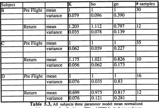
Due to poor data quality, one subject's data could not be reliably analyzed individually. Post flight changes in model parameters were different between subjects. Two subjects exhibited increased 3P normalized model gain post flight (p=.01, p=.06) while one showed a decrease(p=.001). All three subjects showed a decrease in 3P indirect pathway gain (not significant). One subject showed an increase in 10OE gain (p<0.1) and one showed a decrease (p<O. 1). 10OE apparent time constant decreased in all three subjects. A correlation was noted between reported space motion sickness intensity for the subjects, and the magnitude and direction of post flight changes. All three subjects showed significant changes when Et2 statistics were used to compare ensemble averaged pre and post flight data.
Comparison to previous analysis of this data set (Kulbaski, 1988), indicates that the new methods of data filtering and analysis are more effective. Some conclusions from the previous analysis have been overturned while others have been reinforced. Data filtering in the new methods has allowed reliable analysis of individual runs through model fitting.
Individual model fit results have confirmed the variability in individual preflight responses noted by Balkwill (1992) and Oman and Calkins (1993). This may have implications in the clinical testing of the VOR. Average parameters of individual fits show similar changes as the parameters of averaged fits.
The new sk model was found capable of fitting the data well, but was ill suited to this data set. Analysis of sk model parameters showed no significant changes post flight. Suggested improvements in this model could improve its effectiveness at measuring post flight changes. Comparison of the sk model with the 3P and 10E models showed that for analysis of individual run data, better fits to the data were obtained with higher order models (3-4 parameter), than with low order models (2 parameters). However when higher order models are used to fit individual runs, the model fitting routines may also exploit the additional degrees of freedom in an attempt to fit artifacts in the data. This increases the variance of the resulting model parameters.
Thesis Supervisor: Dr. Charles M. Oman
Title: Director
Man-Vehicle Laboratory Senior Research Engineer
Acknowledgments
There are many people that have helped me reach the end of this thesis, but I would first like to thank Jim Costello, for teaching me more than I ever wanted to know about electronics and life. Also thanks go to Dave Balkwill for all the help, even long after he graduated, and being the pathfinder.
For technical help, I would like to thank Nick Groleau for teaching me LabView, Alan Natapoff for helping me with the statistics, and Chuck Oman for the physiology, controls and all the little things that tied it together. Also thanks to Scott Stevenson, and Dan Merfeld for all the helpful discussions of the contents.
Thanks are especially out to Rick Paxon, Mark Schafer and Dave again for showing me that there is life after thesis. Also, Matt Butler, Beave, Pax, Scott, Mark and the rest for reminding me that there is life after midnight, but only across the river. Thanks to all the
MVL lunch crowd; the conversations were the comic relief that kept me (almost) sane. Thanks to Bev, Sherry, Kim, and Christian for keeping the world spinning despite the Gods.
For getting me through all those cold winter weekends, I must thank Dynamic, Salomon, and Tyrolia.
To my family, Mom, Dad, Oma, Jen, and by now Tony, I would like to thank you for all the support you gave me over the telephone. Even on the darkest days you seemed to find some sliver of light.
To Carolyn, I would like to thank you for putting up with me, especially at the end of this thing. Words alone will never suffice...
Thanks also to NASA Contract NAS 9-16523, for supporting this work, and especially for paying my tuition for the last two years.
Table of Contents Abstract 3 Acknowledgments 4 Table of Contents 5 List of Figures 8 List of Tables 9 1. Introduction 10 1.1 Thesis Organization 12 2.0 Background 13
2.1 The Vestibular system 13
2.2 The Vestibulo-Ocular Reflex 15
2.3 Duration of Nystagmus 17
2.4 Testing of Human VOR using Velocity Pulse Stimulation 18
2.5 Velocity Storage Tilt Suppression (Dumping) 19
2.6 Vestibular Models 20
2.7 Effects of Altered GIF 26
2.8 Previous Analysis of SL-1 Data 29
2.8.1 Preliminary Processing 30
2.8.2 Statistical Analysis 31
2.9 Justification for Reanalysis 32
3.0 Experimental Methods 33
3.1 Equipment 33
3.2 Subjects 35
3.3 Experimental Protocol 35
4.0 Data Analysis 38
4.1 New Algorithms for Data Reanalysis 38
4.2 Calibration Procedure 38
4.3 Order Statistic Filtering 39
4.3.1 Predictive FIR Median Hybrid Filter 39
4.3.2 Calculation of SPV using Adaptive Asymmetrical
Trimmed Mean (OS) Filter 40
4.4 Tachometer Analysis 41
4.5 Outlier Removal and Decimation 42
4.7 Individual Model Fits 46
4.7.1 First Order Model Fits 47
4.7.2 Three Parameter Model Fits 47
4.7.3 Sk Model Fits 48
4.8 Dumping Model Fits 48
4.9 Residual Analysis 49
4.10 Mean Model Fits 49
4.10.1 Statistical Comparison of Mean SPV Curves 50
5.0 Results 53
5.1 Calibration 53
5.2 Rejected Runs 55
5.3 Individual Model Fitting 56
5.3.1 Assessment of Model Gain Results 57
5.3.2 Three Parameter Model Directional Asymmetry Analysis 59
5.3.3 Normalization of Data 60
5.3.4 Comparison of Preflight and Post Flight Response 60
5.3.5 Evaluation of sk Model 66
5.3.5.1 Comparison of sk and Three Parameter Models 67
5.3.5.2 Comparison Using Synthetic Data 67
5.3.5.3 Fitting Both Models to real Data 69
5.3.6 Miscellaneous 72
5.4 Analysis of Dumping Runs 73
5.5 Analysis of Ensemble Averaged Responses 78
6.0 New Hardware and Software 85
6.1 Data Analysis Scripts 85
6.1.1 New Algorithms 85
6.1.2 Batch Analysis Scripts 87
6.2 EOG Amplification 89
6.3 LabView Data Acquisition and Chair Control 90
7.0 Conclusions 92
7.1 Trends in Data and Interpretation 92
7.2 Analysis of New Methods 97
7.3 Suggestions for Future Work 101
References 102
Appendix A. Data 105
Appendix C. MatLab External C Codes 126
Appendix D. Batch Analysis Scripts 136
List of Figures
Figure 2.1 Membranous Labyrinth of the right ear, and schematic diagram of one semi-circular canal.
Figure 2.2 Physiology of the otolith organ.
Figure 2.3 Theoretical relative slow phase velocity response to a step in angular velocity.
Figure 2.4 Robinson Model for VOR-OKN interaction for rotations in the dark. Figure 2.5 Raphan-Cohen model of OKN, OKAN, and Vestibular Nystagmus. Figure 2.6 Five parameter modified Laplace Transfer Function Model for
rotation in the dark without left-right asymmetries. Figure 2.7 Simple first order model (10E) for nystagmus decay Figure 2.8 SpaceLab SL-1 grouped mean post-rotatory SPV Figure 2.9 SpaceLab D-1 grouped mean post-rotatory SPV Figure 3.1 Experimental set-up
Figure 5.1a Normalized Three Parameter Model gain, K, for all subjects, both CW and CCW, per and post rotatory.
Figure 5. l1b Normalized Three Parameter Model ho, for all subjects, both CW and CCW, per and post rotatory..
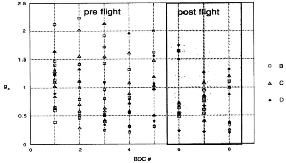
Figure 5. 1c Normalized Three Parameter Model go, for all subjects, both CW and CCW, per and post rotatory.
Figure 5.2a Normalized first order model gain, K, for all subjects, both directions, per and post rotatory.
Figure 5.2b Normalized first order model time constant, T, for all subjects, both directions, per and post rotatory.
Figure 5.3 Comparison of sk and three parameter models
Figure 5.4 sk and three parameter model fits to the C203 post-rotatory data Figure 5.5 Residuals of C203 post-rotatory model fits between sk model
and data, between three parameter model and data, and between models
Figure 5.6, C304 log-linear fits to before dumping region, dumping region, and after dumping regions
Figure 5.7 C205 log-linear fits to pre-dumping region, dumping region, and post-dumping regions
Figure 5.8a Subject B, Mean dumping model slopes Figure 5.8b Subject C, Mean dumping model slopes Figure 5.8c Subject D, Mean dumping model slopes
Figure 5.9 Subject B ensemble averaged preflight versus post flight Figure 5.10 Subject C ensemble averaged preflight versus post flight Figure 5.11 Subject D ensemble averaged preflight versus post flight Figure B1 DAM/DQML-mod6 front panel
Figure B2 Run/Cal front panel. Figure D1 Batch_analysis flow chart
14 15 19 21 22 22 23 27 28 33 61 61 62 62 63 68 70 70 74 75 76 76 77 79 79 80 124 125 138
List of Tables
Table 5.1a Run rejection status for subject A 55
Table 5.1b Run rejection status for subject B 55
Table 5. 1c Run rejection status for subject C 56
Table 5. ld Run rejection status for subject D 56
Table 5.2 Summary of directional asymmetry t-test results 59
Table 5.3 All subjects three parameter model mean normalized
model parameters 65
Table 5.4 All subjects first order model mean normalized
model parameters 65
Table 5.5 All subjects two-tailed t-test results 66
Table 5.6 Synthetic data generation parameters and model fit
parameters from figure 5.1 68
Table 5.7 Model fit parameters for sk and three parameter models to
C203 post-rotatory data 69
Table 5.8 Ensemble averaged model fit parameters for each subject 81 Table 5.9 X2 results for pre and post flight head up ensemble averaged
SPV curves 82
Table 5.10 sk model fit parameters to ensemble averaged data 83 Table 5.11 Two parameter sk model fits to ensemble averaged data 84 Table 7.1 Apparent time constant for ensemble averaged runs as found
previously (Kulbaski, 1988). 94
Table 7.2 Apparent time constant for ensemble averaged runs as found
in this study. 94
Table A. 1 a Horizontal calibration factors for subject A 106
Table A. lb Horizontal calibration factors for subject B 106
Table A. lc Horizontal calibration factors for subject C 106
Table A. id Horizontal calibration factors for subject D 106
Table A.2.1 Subject B per-rotatory model fit parameters 107
Table A.2.2 Subject B post-rotatory model fit parameters 108
Table A.3.1 Subject C per-rotatory model fit parameters 109
Table A.3.2 Subject C post-rotatory model fit parameters 110
Table A.4.1 Subject D per-rotatory model fit parameters 111
Table A.4.2 Subject D post-rotatory model fit parameters 111
Table A.5a Dumping log-linear model fits for subject B. 112
Table A.5b Dumping log-linear model fits for subject C. 112
Table A.5c Dumping log-linear model fits for subject D. 113
Table A.6.a Per rotatory sk model fit parameters for subject B. 113 Table A.6.b Post rotatory sk model fit parameters for subject B. 114 Table A.7.a Per rotatory sk model fit parameters for subject C. 114 Table A.7.b Post rotatory sk model fit parameters for subject C. 115 Table A.8.a Per rotatory sk model fit parameters for subject D. 115 Table A.8.b Post rotatory sk model fit parameters for subject D. 116
1. Introduction
As spacecraft have grown larger, from the small Mercury and Gemini vehicles, to the larger Sky-Lab and Space Shuttle in the US fleet, most astronauts have begun to experience a physical discomfort upon entry into the micro gravity environment, known as space motion sickness (SMS). First reported by cosmonaut G. Titov in 1961, approximately 60% of both American and Soviet crews experience some symptoms of
SMS while in micro gravity. The symptoms of SMS are similar to motion sickness on earth; pallor, sweating, lethargy, nausea and vomiting. The symptoms experienced by any individual vary, but generally decrease and disappear over the course of two to five days. Due to the great expense of space flights, the lost productivity of crew members due to SMS is of considerable concern, as are long term adaptation effects which could impact on longer space flights, such as the proposed manned Mars mission.
On the earth, The human body is subjected to a constant gravito-inertial force (GIF) caused by Earth's gravitational field, equaling 9.81 m/s2. The human brain processes information from its sensory systems (vestibular, proprioceptive, and visual) with knowledge of this 1-G bias in order to determine position and orientation. When the body is subjected to a GIF different from that to which it is accustomed, the body is forced to adapt the sensori-motor systems for the new environment. Adaptive change in the CNS processing of sensori-motor systems can result in symptoms similar to SMS . This has been seen in centrifuge studies (Guedry and Benson, 1978) and parabolic flight (Lackner and Graybiel, 1984) where the GIF acting on the body is changed.
The sensory conflict theory of SMS states that when conflicting information is passed to the central nervous system (CNS) by the sensory systems, the CNS is unable to convert the sensory information into a recognizable body orientation, resulting in physical
discomfort and illusions. If the unusual gravitational force persists, the CNS is able to adapt by creating new internal models with which to interpret body position. Thus,
symptoms decrease and disappear eventually as the unusual conditions persist.
In order to study this phenomenon, a set of experiments have been designed and performed in a series of space shuttle SpaceLab flights including the SL-1 (1983), D-1 (1985) and SLS-1 (1991) missions and the upcoming SLS-2 mission (1993). This thesis work is a re-analysis of one of these experiments from the SL-1 mission, the use of a rotating chair to identify the dynamics of the horizontal angular vestibulo-ocular reflex (VOR). Experiments were performed on five crew members preflight and four crew members post flight, after micro-gravity adaptation had occurred. Analysis of the D-1 data and previous analysis of the SL-1 data (Kulbaski, 1986; Oman and Wiegl, 1989) has shown some changes in how the CNS interprets sensory information after adaptation. However, new methods in data filtering and analysis, and the use of more complex models justifies re-analysis of the SL-1 data (see section 4.2).
The SL-1 data was compared against two mathematical models of the vestibular system to quantitatively determine the changes in the CNS after adaptation. A third VOR model was developed and compared to the existing models to assess its strengths and weaknesses. A new data acquisition and chair control system was developed, and the existing analysis algorithms were automated, and, in some cases improved, to allow rapid, on-site data processing and preliminary analysis on future missions.
1.1 Thesis Organization
Chapter 2 presents the physiology and previous research into the human vestibular system. Various models of the vestibular system are discussed.
Chapter 3 describes the experiment protocol and data acquisition.
Chapter 4 describes algorithms used in previous analysis of the SL-1 data, provides justification for reanalysis and describes the new algorithms developed.
Chapter 5 presents the results of the data analysis.
Chapter 6 introduces new software and hardware developed for future missions.
Chapter 7 is a discussion of the implications, and conclusions based on the data analysis. Also, recommendations for future work are included.
2.0 Background
The basis of human orientation is reflexive, and seldom is it consciously noted or controlled. Orientation is determined through CNS processing of the various sensory inputs available to it. This information is used to maintain balance, as well as awareness of the relative positions of limb and body. Visual and vestibular cues are used to stabilize vision in the presence of head movements. Vestibular information is used to stabilize vision during rapid head movements, while retinal slip helps to stabilize vision during
slow head movements, or steady state.
2.1 The Vestibular System
For a complete reference on the vestibular system, refer to Wilson and Jones, 1979.
The vestibular labyrinth is the location of the body's sensors of angular motion, linear motion, and gravity. Angular motions are sensed by the semi-circular canals while linear motions are sensed by the otolith organs. Each labyrinth comprises three canals, lying approximately orthogonal to each other, and two otoliths oriented horizontally (utricular otolith) and vertically (saccular otolith). The canals are arranged such that they are tilted approximately 20' back from the horizontal. The canal which lies closest to the horizontal plane is referred to as the horizontal semi-circular canal.
Each semicircular canal is composed of a semicircular duct, filled with endolymph fluid. In each duct, there is a diaphragm composed of gelatinous tissue which is attached to the ampula much like a drum skin. When the head is rotated in the plane of the semicircular canal, the inertia of the endolymph causes it to lag behind the head. This gives a relative motion between the endolymph and the head, which causes the cupula to deform, and a corresponding deflection of cilia of the sensory cells which are attached to the cupula. The deformation in the cilia causes a change from the resting firing rate of the sensory
cells. The change in the firing rate is proportional to cupula deflection and therefore head angular velocity, and is direction dependent. For large stimuli, the firing rate can saturate. The tension in the cupula and ampula causes a restoring force which accelerates the endolymph, and returns the cupula to the resting position. The cupular motion can be approximated by a highly damped torsional pendulum.
Superior omloircula
ampulls of
lateral micircular cwn
semicircular
canal endolymphatic duct
cochlear nervi
potaior
micircular cochle
utrile spire lion
Figure 2.1, Membranous Labyrinth of the right ear, and schematic diagram of one semi-circular canal showing the relationship between head rotation and cupula deflection. Actual deflections are very small.
[from Laurence Urdang, 1982, and Benson 1967]
Within the vestibule lie two large membranous sacks, part of the labyrinth, known as the utricle and saccule. Within each of these cavities lie the body's linear accelerometers, the otoliths. The sensory part of the cavities is called the macula. This consists of ciliated sensory cells covered by the otolithic membrane, and a calcium carbonate deposition in the membrane. These calcium crystals have a density approximately three times that of the surrounding endolymph, so when the head is subjected to a linear acceleration, the crystals lag behind the surrounding endolymph, shearing the crystals relative to the macula, bending the cilia and thereby causing the sensory cells to change their firing rates (Fernandez and Goldberg, 1976). Due to the equivalency of gravitational force and acceleration (Einstein equivalence principle) , the otoliths respond to changes in the
orientation and magnitude of the GIF as well as to linear accelerations and head rotations. Since the macula of the saccule lies in a predominantly vertical plane, gravity induces a bias in the resting position of the saccular macula. During exposure to micro gravity, the saccular otoconia are unloaded, removing the 1-G bias, and changing the resting firing rate of this macula. Pitch and roll head rotations in micro gravity will no longer cause the otoliths to sense a changing GIF, while centripetal forces due to head rotations and linear accelerations will still stimulate the otoliths normally. Thus, the otoliths will no longer give information on the orientation of the head to an external reference (i.e.
Otoconia
Macula
Sensory Cells
Utricular or Saccular Nerve
Figure 2.2, Physiology of the otolith organ. [from Wilson and Melvill Jones, 1979]
gravity) and the CNS must adapt to the absence of this signal.
2.2 The Vestibulo-Ocular Reflex
When you are looking at some target, and make a head movement, your eye must compensate by rotating the opposite direction to maintain a stable image on the retina.
For steady state gaze, and slow head movements image stabilization can be accomplished by the CNS by minimizing retinal slip. For fast head movements, the visual processing of retinal slip is too slow (about 70 msec) to stabilize the image, and the vestibular system is used to generate the requisite compensatory eye movements. This is called the vestibulo-ocular reflex (VOR). The VOR relies on the semicircular canals and otoliths to provide information on how the head is moving, and uses this to rapidly (about 10 msec latency (Robinson, 1975)) generate compensatory eye movements to prevent retinal slip, while retinal processing is used to correct small error remnants.
When head rotations are large or continuous, the magnitude of the required compensatory eye movements exceeds the physical limitations of eye rotation. When this happens, the eye will make a fast jump in the direction of motion, known as a saccade, and then continue tracking from this new position. For very long or continuous rotations, the eyes will saccade forward after they have counter rotated back past the center position, maintaining eye position biased towards the direction of rotation. A series of these saccades with reflexive slow tracking between is known as optokinetic nystagmus (Komatsuzaki et al, 1969). During nystagmus, the saccades are generally referred to as fast phases, while the tracking portion is referred to as the slow phase. The eye velocity of the slow phases (SPV) is equal to the velocity of the visual scene relative to the head, when a visual scene is presented to the subject. During rotations in darkness however, there is no longer a retinal slip signal from the eyes to fine-tune the eye movements, and the CNS relies entirely on vestibular information. Thus the eye movements are only due to the VOR. For long or continuous rotations in darkness, the nystagmus that is generated is known as vestibular nystagmus.
VOR is capable of being consciously modified by subjects rotating in the dark (Barr et al, 1976). When subjects were asked to imagine and stare at a point rotating with them in
front of their faces, they are able to partially suppress the VOR. Provided with a real point to fixate on, subjects can almost totally suppress the VOR. Level of mental alertness also affects VOR (Collins, 1962). Low levels of alertness also cause partial suppression of the VOR. Thus it is very important to properly and instruct subjects prior to testing.
2.3 Duration of Nystagmus
Through direct single unit neuron recordings in monkeys (Raphan et al, 1979), it has been seen that the firing rate of the sensory canal neurons during continuous rotation in the dark returns to the resting rate before nystagmus ceases. The deviation from the resting firing rate follows an approximately exponential decay with a time constant of approximately 5 seconds, while nystagmus decay follows a time course with a decay time constant closer to 20 seconds. From this, it has been hypothesized that there exists an element in the CNS that stores the sensory information from the canal afferents to prolong nystagmus. This is commonly referred to as velocity storage. From an evolutionary standpoint the existence of velocity storage would serve to aid the CNS in properly evaluating rotations that persist longer than the time constant of the cupula, when the vestibular system equilibrates and indicates no motion when in fact a steady state rotation has been achieved. Studies in optokinetic after nystagmus (OKAN) also support the theory of a velocity storage element. OKAN occurs when an immobile subject is exposed to a moving visual field which induces nystagmus. After the scene is stopped, nystagmus persists, which indicates the presence of a storage element.
Current theory holds that the source of velocity storage mechanisms in the brain is in the flocculus of the cerebellum, where vestibular, visual and proprioceptive cues are integrated. However, to date anatomists have been unable to determine the location of the velocity storage element, although recordings in the vestibular nucleus have found both
the afferent neuron signals from the vestibular system as well as units with signals corresponding to canal signals modified by the additional velocity storage element.
2.4 Testing of Horizontal VOR using Velocity Pulse Stimulation
Several tests of the human horizontal VOR have been developed. While various sorts of rotational stimuli are commonly used, only velocity pulse stimuli will be discussed here.
To test the human horizontal VOR, the subject is seated upright in a rotating chair, and rotated about the vertical axis. In order to isolate the VOR, sensory cues other than from the VOR are masked out by rotating in the dark with auditory and proprioceptive cues removed through the use of earphones and long clothing to eliminate wind cues.
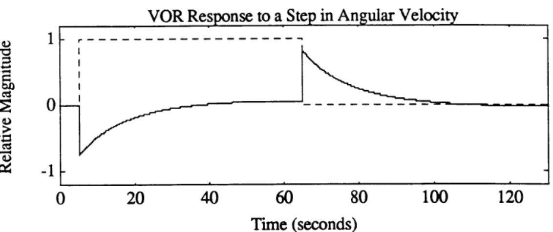
Subjects are subjected to a step in horizontal angular velocity . At the beginning of the stimulus, the VOR drives a rapid rise in SPV to a maximum usually between 0.5 and 0.8 of the stimulus velocity in the opposite direction to compensate. The cupula returns to its initial position rapidly, and the primary afferents return to their resting firing rate due to the absence of any angular acceleration at the constant rotation. Velocity storage prolongs the SPV of the eye movements which decay approximately exponentially to zero after 40 seconds. In humans and animals, often the SPV decay will "overshoot", briefly reversing nystagmus, giving SPV in the same direction as the stimulus with low magnitude. This is thought to be a result of neural adaptation, and has a time constant on the order of approximately 80 seconds. When the rotation is then stopped, an equal but opposite angular acceleration is induced in the canals causing nystagmus in the opposite direction with equal magnitude. The subject subjectively interprets this period as a rotation in the opposite direction although they are immobile. Figure 2.3 shows a typical SPV response to a velocity step input, calculated using a five parameter model (section 2.7).
-1
0
-
--0 20 40 60 80 100 120
Time (seconds)
Figure 2.3 Theoretical relative slow phase velocity response to a step in angular velocity. Solid line is SPV response. Dashed line is stimulus. Calculated using a five parameter model (Balkwill, 1992)
2.5 Velocity Storage Tilt Suppression (Dumping)
If, immediately following the cessation of rotation of a velocity step, the head is pitched forward, the CNS will receive conflicting information from the otoliths and canals. Following chair stop, the canal afferents signal the CNS that they are rotating in yaw. After the head is pitched, this is translated to an apparent rotation in roll in body axes coordinates. Meanwhile, the otoliths are recording a steady GIF, whereas if the head were rolling, the GIF would be changing relative to the otoliths. Other senses, such as the proprioceptors also indicate that no roll is taking place. This conflict persists until the cupula returns to its steady state position. The SPV response during this period has a characteristically faster decay approximating that of the canal time constant alone. It is theorized that in the presence of the conflicting information coming from the canals and otoliths, the CNS suppresses, or dumps the information in the velocity storage element. Presumably, the CNS realizes that it no longer has a reasonable estimate of body orientation, and is attempting to develop a new estimate from "scratch". Information from the velocity storage element is suppressed, not lost, for if the subject returns to the upright, the SPV time course will sometimes return to the appropriate velocity as if the head had remained upright continuously (Kulbaski, 1986).
An alternative theory of what happens during "dumping" is called axis shifting. As the head rotates forward, the CNS keeps track of the eye movements in global coordinates. While the head is pitched down, the CNS calculates the axis of rotation between the original vertical axis and the new horizontal axis. Eye movements are shifted accordingly, reducing horizontal nystagmus while beginning torsional nystagmus. Experiments in monkeys have shown some evidence of axis shift during passive head movements (Merfeld, 1990), however recent experimentation in humans has shown no evidence of axis shift following active head movements (Fetter et al, 1992 in progress).
2.6 Vestibular Models
As this thesis is primarily concerned with modeling the human horizontal angular VOR, the inputs and outputs of each model are chosen to be the rotational velocity stimulus, and the eye SPV respectively. The following models have several differences between them, but there are several areas in which they are in agreement. The dynamics of the semicircular canals are modeled in each case as a low pass filter on head angular acceleration, giving head velocity as output over a mid-frequency range. All three models assume implicitly at least, that the brain uses an internal model of SCC dynamics. It is this model that generates the brain's best estimate of head velocity based upon the most recent sensory inputs. In the absence of new information, such as during prolonged rotation, the model continues to update the estimate of body rotation based upon its model of the dynamics.
The characteristics of the VOR are commonly modeled using engineering controls methods designed for linear systems. In general, Laplace transform methods will be used here to describe the models.
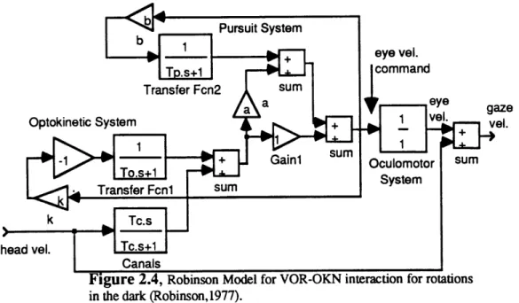
The Robinson model (Robinson, 1971) is based on the idea that the sole purpose of the VOR-OKN system is to provide a signal proportional to head velocity for low frequencies where the canals are ineffective (see figure 2.4). The positive feedback loop of eye velocity command (upper feedback loop in figure 2.4) gives the system the high forward gain and long time constant to mimic velocity storage. In the dark, this will increase the main VOR time constant from Tc to Tapparent, the apparent time constant of the VOR. bPursuit System + eye vel. T.s+1command Transfer Fcn2 sum a eye gaze
Optokinetic System + vei. vel.
Gain1 sum
-1 + Gain Oculomotor sum
System Transfer Fcn sum
k Tc.s head vel. Tc.s+1
Canals
Figure 2.4, Robinson Model for VOR-OKN interaction for rotations
in the dark (Robinson, 1977).
The Raphan-Cohen Model (Raphan et al, 1977) is shown in figure 2.5. This model takes into account all of the characteristics of the VOR mentioned above. The Raphan-Cohen model can be simplified and rendered into Laplace notation using some simplifying assumptions. First, rotation in the dark allows the neglect of the visual portion of the model. Second, we assume that the system is left-right symmetrical, allowing removal of the direction asymmetry terms. Next, cupula dynamics are assumed to be a simple exponential decay with a gain K, and time constant, Tc. Finally, adaptation
effects are treated as another exponential decay in series with the cupula (Fernandez and Goldberg). This is here referred to as a five parameter modified Raphan-Cohen VOR
model or more simply, the five parameter model(Balkwill, 1992) (see figure 2.7). In this thesis, the five parameter model is used with Ta and Tc frozen at values of 80 and 6 seconds respectively. This is referred to as the three parameter (3P) model.
Direct Vestibular Pathway Head
Velocity.
Output
ye velocity)
Figure 2.5, Raphan-Cohen model of OKN, OKAN, and vestibular
nystagmus (From Raphan et al, 1979).
eye velocity
head velocity
Canal Dynamics Neural Adaptation
Sum1
Indirect
Pathway Gain
Leak rate
Figure 2.6, Five parameter modified R-C Laplace Transfer Function
Model for rotation in the dark without left-right asymmetries.
In this model, the eye velocity signal is a sum of the activity in both the direct and indirect pathways. One major difference between this model, and the Robinson model, is that the storage effects of the system are modeled as efferent feedback in the Robinson model, whereas the modified Raphan-Cohen model assumes that the integrator
represents a separate state of the system, and models this using feed forward. A significant feature of the modified Raphan-Cohen model, is that the zero associated with the indirect pathway is believed to cancel the canal pole. Thus, as with the Robinson model, the response can be approximated by a single apparent time constant that lies between the adaptation and indirect pathway time constants.
Both the Robinson and modified Raphan-Cohen models can be simplified to a simple first order model representation (10E model). This consists of a first order lag, with a gain and time constant to describe the decay of horizontal nystagmus in the dark (see figure 2.7). The time constant can be likened to the apparent time constants of the previous models. An apparent time constant is the time constant of a first order equivalent system to a higher order VOR model. It does not represent the dominant time constant of the higher order model, but is influenced by both time constants.
angular velocity > SPV
>Ta.s+l
Gain Simple Lag
Figure 2.7, Simple first order model (10E) of nystagmus decay.
An alternative model is based upon work carried on the semicircular canal afferent fibers of the pigeon (Landolt and Correia, 1980). This model, here referred to as the sk model, uses a different method to express the effects of canal adaptation. Canal afferent response to accelerations can be modeled with a transfer function of the form,
H(s) = Gsk 1 1
(,Ls + 1) (rss + 1)
Here, the parameter G represents the system gain, k is an adaptation constant ( 0<k<l ), and rL and Ts are the long and short time constants of the torsion pendulum model of the cupula. The term s k can be decomposed into a series of polynomials in s of the form;
sk C Jiris
A single term equivalent to this expansion, C' Ji ri s / ( 'ris + 1) is similar to the neural
adaptation term found in the five parameter model above. The C' term is a magnitude adjustment for reducing the infinite sum to a single term. The Ji term is the value of a probability density function, J(T), evaluated at r = r . The Probability density
function (Thorsen and Biederman-Thorsen, 1974) has the form; S 1
k+1
Lz
for all r > 0
This has the effect of amplifying fast acting time constants the most, and long time constants very little. As the fractional Laplace operator (sk) was originally developed for use with visco-elastic materials, there is an analog to these we can use (Gross, 1953). For a fast acting force/response, the material behaves elastically like a spring. For slower force/response, the material relaxes, or creeps. One significant feature of this relaxation spectrum for vestibular modeling, is that for the longer time constants, the Ji term is much smaller than for shorter time constants, and thus faster time constants are more heavily weighted in the overall response.
Due to its small effect on the response (two orders of magnitude below the (,L s + 1)-1 for the frequency range concerned here), the (, rs + 1)- 1 term was ignored in this model,
simplifying it to;
H(s) = Gsk
( rs + 1)
Given an input acceleration impulse stimulus of amo/second the model response in the time domain becomes;
r(t)= (G )[y*(-k,- )e- ]
y*(a,x) = e x x tale'dt V(a) o
is the incomplete gamma function (which is single valued and finite in terms of a and t) and T(a) is the complete gamma function evaluated at a. At negative values of t, for -1< a <1, the incomplete gamma function can be evaluated using the following series;
y*(a,x)= 1 1+a "
*(a,x) = F(1 + a) [i + (n + a)n!where y =
txI
To change this from a canal model to a VOR model, velocity storage terms, using the same notation as for the five parameter model, were added. This gives the VOR model transfer function as;
H(s) = GskS A + h}
,rS+1 S+h
1- rL(go + h)
A=Y-h
B=- 90
The time response of this system to an acceleration impulse may then be written as r(t) = ( )[Ay * (-k,- )e- L + By * (-k,-hot)e"' ]
This model will be referred to as the sk model although it also incorporates VOR velocity storage effects.
Motivation for the use of this model arises from Correia, et al (1992). Correia found that following 14 days of space flight, two Rhesus monkeys showed increased gain and adaptation in SCC afferents. This suggested that one or more components of the vestibular end organ was transiently modified following space flight, and that the sites of
plasticity of vestibular responses may not be exclusively within the CNS. The modified Raphan-Cohen models do not predict gain changes due to changes in peripheral neuron adaptation. The sk model accounts for neural response changes through the k parameter, which affects both gain and apparent time constant.
2.7 Effects of Altered GIF
Early tests of VOR response in centrifuge have shown, that the magnitude and duration of nystagmus was shorter when the head was reclined during a GIF greater than one. Later testing in parabolic flight (DiZio and Lackner, 1988) has shown that the apparent time constant of decay in both O-G and 1.8-G is significantly shorter than it is in 1-G. Active head movement provoked velocity storage dumping was observed in both the 1-G and 1.8-G trials, but not in the 0-G trials. This implies that the presence of an altered GIF magnitude is equivalent to the dumping head movement, which alters the direction of the GIF, in provoking velocity dumping in humans.
Adaptation to altered GIF has been studied previously as part of the D-1 and SLS-1 SpaceLab missions. Also, there has been some previous examination of the SL-1 data presented here.
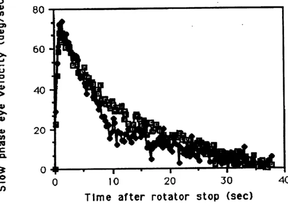
Previous analysis of the SL-1 data (Kulbaski, 1986) was confined to SPV responses averaged across all subjects and all five pre-flight data sessions versus the first two post-flight sessions (refer to section 3 for a description of the SL-1 experiment). A first order exponential model was fit to the first twenty seconds of averaged head up data, and t=5 to t=10 of dumping head movement data. This analysis found that while the head up time constant decreased significantly after exposure to micro-gravity (11.7 seconds pre-flight versus 9.3 seconds post-flight), the gain ( 0.60 pre-flight versus 0.59 seconds post-flight) and the dumping time constants (3.2 seconds pre-flight versus 3.4 seconds post-flight)
were unchanged . x2 analysis showed significant differences existed between the head up runs pre and post-flight from 6 to 20 sec after stop, and between the head up and dumping runs from 5 to 10 seconds after stop. SL-1 post-rotatory SPV averaged across subjects are shown in figure 2.9. It was believed that the change in pre-flight versus post flight responses, while there was no change in dumping responses, was due to two reasons; first, in the altered GIF environment of space, the CNS had partially suppressed the VOR velocity storage as a result of altered GIF, and second, over the time in flight, the CNS adapted to this altered GIF, and remained so for a short period post-flight. Because tilt suppression still occurred following exposure to micro gravity, there was no
evidence that the otoliths were ignored by the CNS following exposure to micro
U u 0 Q U) r 41, '~i 41 U)
80
60
40
20
0
0
10
20
30
Time after rotator stop (sec)
40
Figure 2.8 SpaceLab SL-1 grouped mean post-rotatory SPV
gravity, and thus further tilt suppression beyond the adaptive tilt suppression was still possible.
On the D-1 mission, (Oman and Weigl, 1989), horizontal VOR was tested in five SpaceLab crew members 4 times pre-flight and five times post flight. Two of the subjects were directionally asymmetrical, while the other three subjects showed no change in VOR gain, and a more rapidly decaying SPV response post-flight then pre-flight. A X2 analysis showed a significant difference in the post-flight versus pre-flight at the p < .001 level. D-1 post-rotatory SPV averaged across subjects are shown in figure 2.8. 80 70 60 50 40 20 10 40 0 10 20 30
TIME (sec)
Figure 2.9, SpaceLab D-1 grouped mean post-rotatory SPV
pre-flight (squares) versus post-pre-flight (circles). 0 3 0 *
8
* Qe'1 o 9 ar e Ib,On the SLS-1 mission (Balkwill, 1992), four crew members were tested on four days pre-flight, and four days post-flight. The subjects were rotated at 120 */second for sixty seconds while seated upright. The chair was stopped and the subjects remained upright for half the runs, and pitched their heads forward 90* after chair stop, for the other half. The dumping protocol was changed from the SL-1 and D-1 missions, in order for two reasons. First, this allowed a full sixty seconds of dumping data to be collected and modeled for changes, and second, as there is some uncertainty as to whether nystagmus suppression stops completely following return to the head erect position, analysis of post-dumping sections of previous data sets had been excessively complex. For SLS-1, the SPV was calculated, and fit to the five parameter modified Raphan-Cohen model (see section 2.6), and subjective duration of rotation was recorded. The apparent time constant of decay of the SPV was found to be lower post-flight than pre-flight, suggesting adaptation within the velocity storage mechanism. The change was believed to be a result of changes in indirect pathway gain on the model. Subjective responses were also found to be significantly shorter post-flight than pre-flight for three out of four subjects. For use on the SLS-1 and subsequent missions, new methods of analysis were developed including the use of order statistic filtering, automated dropout and outlier removal, iterative model fitting techniques, and Xt2 testing (Balkwill, 1992).
2.8 Previous Analysis Methods used on SL-1 Data
Previous analysis of the SL-1 rotating chair data set was carried out in 1986 by Mark Kulbaski. Following digitization of the data, three data processing steps were carried out; SPV was determined, manual SPV editing was performed, and data was resampled at 4 Hz for statistical analysis.
2.8.1 Preliminary Processing
The SPV was calculated using the acceleration based Massoumnia algorithm (Massoumnia, 1983). The algorithm first differentiated the angular position signal to get angular eye acceleration. The algorithm then used a set of rules based on eye acceleration to classify each eye movement as either a fast phase or a slow phase of Nystagmus. Fast phase movements were replaced with a linear interpolation between adjacent slow phases. The Massoumnia algorithm occasionally failed to properly classify eye movements, and
thus fast phases that were not removed had to be removed through manual editing.
Misclassification was due to several causes. One was that the low pass filters rounded out the peaks of high amplitude nystagmus preventing the algorithm from detecting the fast phase. A second cause was when the algorithm correctly determined a fast phase, but failed to accurately determine its beginning and end before interpolating across it. This was interpolated at an incorrect velocity as the interpolation would be between transition phases instead of slow phases. A third cause of errors was associated with transients in the EOG signal. There were two typical sources of transients: When the head tilted down during dumping runs, an electrode motion artifact occurred during each pitch movement. Also whenever the amplifier DC offset was manually adjusted to compensate for electrode drift, a transient was injected into the EOG. Finally, if the signal to noise ratio of the signal was low, the noise would confuse the algorithm, and it would completely fail to detect phases correctly.
Manual editing was performed on a PDP-11 using an interactive program known as SPARTA (Digital Equipment Corp., Maynard, MA). The program read the SPV file from the Massoumnia algorithm, and displayed the SPV on a CRT. Using potentiometers, the user positioned two cursors on the screen to mark the beginning and end of a fast phase. The data between the cursors was replaced with values linearly
interpolated between the values at the marked points. Following manual editing, the SPV files were resampled to 4 Hz before further processing.
Of the 145 runs analyzed, 21 of them were then discarded at this point on the following basis. If there was an abrupt change in the noise level in the EOG signal, this would suggest an electrode had lost contact. If an EOG signal had a low signal to noise ratio, the Massoumnia algorithm would fail to determine the SPV profile. If the SPV profile was markedly atypical the run would be discarded. If the SPV response lagged significantly behind chair motion, this indicated that the subject wasn't paying attention. In all of these cases, the runs were discarded. However, all criteria were only semi-quantitative.
2.8.2 Statistical Analysis
Two forms of statistical analysis were performed. The first was to conduct a X2 analysis to determine if two response curves were different. The second was to fit a simple exponential model to the data, and then to use ANOVA and t-tests to determine if the model gain and time constant were significantly different.
The CW and CCW responses were tested by X2 to determine if responses were directionally symmetrical. As no directional asymmetries were found, the CW and CCW runs were normalized for direction and averaged together. X2 analysis was performed to determine whether there was a trend across test days for all subjects. As no trend was determined, all pre-flight data was averaged together for each subject, and the first two post-flight sessions were averaged together for each subject. However this left the possibility of trends within individual subjects, which was not tested. Subsequently, Balkwill (1992) noted that Kulbaski had actually calculated the Yt2 statistic and assumed that it followed the X2distribution, which is not valid for small n.
Model fits were performed on averaged data sets for each subject using a simple exponential model. This was carried out through the use of a log-linear least squares fit to the data over the first twenty seconds of data for PRN and per-rotatory portions, and from 5-10 seconds after the chair stop for dumping runs.
Results from this analysis were reported in chapter 7.
2.9 Justification for Reanalysis
Previous analysis of SL-1 data had several weaknesses. First, the manual SPV editing was a potential source of error. Manual editing is always subject to variability due to human inconsistencies, and therefore standards for selection of edited portions on different runs may have varied. Also, the edited data was included in all subsequent processing even though the actual data had been replaced by an interpolated line. Thus interpolated points were inserted into the data at the interpolation regions that was then used for calculation of run statistics. Another weakness is the use of only semi-quantitative run exclusion criteria. A third weakness is that no individual runs were fit; all analysis was performed on data averaged over several trials. Analysis of individual runs would allow extraction of the variability of the responses. Individual and day to day variations were smoothed over by averaging. Through analysis of individual data, trends within subjects become much easier to see, where they are hidden by the averaging process and other analysis such as ANOVA become possible. A third weakness was the limitations of the model fit to the data. Only simple exponential models were fit to the data, and velocity storage was not modeled. New insight might be gained through re-analysis of this data using newer models such as the five parameter model and sk models. Further justification for reanalysis is that new methods in EOG signal filtering have been developed (Balkwill, 1992) that can be used to improve the data quality.
3. Experimental Methods.
3.1 Equipment
The experimental apparatus was composed of the equipment used for the NASA Spacelab E072 F02 rotating chair experiment. This consisted of a motor driven rotating chair, and EOG data collection equipment.
The rotating chair (see figure 3.1) was constructed as an undergraduate thesis project by MIT students for use in the SL-1 and subsequent experiments (Johnson and Gidney, 1983). The chair was driven by a .75 hp, 27 ft-lbs torque DC motor, capable of smooth rotation of the chair at angular velocities up to 200'/sec. An Inland Motor Division TPA series motor controller and tachometer provided closed loop control of motor speed. The velocity control command was generated by a voltage across a potentiometer which was dialed by hand. Chair stop was initiated by grounding the velocity command using a toggle switch, which generated approximately a step velocity change.
Rotating Chair
FM Tape Instrument Recorder
WCommand Generation
Rotating Chair Base and Filter Box (Motor + Controller)
Data collection was accomplished through the use of electro-oculography (EOG). Five infant cardiac electrodes were placed above and below the right eye, on the left and right temples and either at the center of the forehead. The eye position was determined through measuring the relative voltage between pairs of electrodes. Since the eye has a dipolar magnetic field associated with its cornea (the corneo-retinal potential), movement of the eyes changes the induced voltages across electrode pairs, allowing eye position to be determined. The electrode pair at the temples monitored horizontal eye position, the electrode pair above and below the right eye monitored vertical eye position, while the fifth electrode was used as a reference ground for common mode rejection. Variability induced by inexact electrode placement and changing corneo-retinal potentials, was removed through calibration of the EOG using targets at known positions relative to the head. Electrode leads were connected to a differential amplifier (nominal gain 3000) mounted on the chair seat. Amplifier output was two voltage signals corresponding to horizontal and vertical eye position, with magnitudes between ± 15 volts. A manually controlled DC offset was added to these signals in the amplifier in order to keep the signals within ± 10 volts. The position voltage signals were passed through slip rings at the base of the chair shaft to the chair panel, and then through three cascaded first order analog low pass filters with corner frequencies at 30 Hz. Filtered EOG signals and the tachometer signal were recorded analog on FM tape using a calibrated Hewlett Packard
3964A Instrumentation Recorder.
The data was digitized in the MIT Man-Vehicle Laboratory (MVL) in two batches. The first batch consisted of all pre-flight runs, and post-flight runs for subjects A, C, and D. This was digitized from the FM tape using the same FM recorder playing into a Macintosh Mac II computer running the Labtech Notebook version 1.0.1 software package, sampling at 120 Hz. The output range of the recorder was limited to ± 3 volts, and for this batch of data, input range on the Mac II A/D board was set to ± 10 volts.
The second batch of data consisted of all subject B post-flight runs. This was digitized using the Labview version 2.1 software package sampling at 120 Hz. For this batch, A/D input range was ± 1 volt, with the recorder output being adjusted to ± 1 volt. Both batches were saved in identical binary form and all further processing was identical.
3.2 Subjects
Subjects used in this experiment were all members of the SL-1 crew team. Six subjects were tested preflight, including the four SL-1 payload specialists and two alternate payload specialists. Post flight testing was only conducted on the four payload specialists, as the alternate payload specialist did not fly on the mission. All subjects tested were male and all were free of any overt vestibular disease. To preserve confidentiality, flight subjects were assigned the code letters A, B, C and D and will be referred to as such herein.
Subjects were tested on five separate days before the flight. The pre-flight tests were performed on F-151, F-121, F-65, F-43, and F-10 days before launch. Post-flight testing was conducted on three days after recovery, R+1, R+2, and R+4 days after landing. All experiments were performed at the NASA Dryden Research Facility at Edward's Air Force base, California, by Dr. Oman.
3.3 Experimental Protocol
The same protocol was used for each subject on each test day. Deviations from this protocol are noted at the end of this section.
The subjects were seated upright in the rotating chair with their heads directly above the axis of rotation. Prior to electrode placement, the subjects skin was cleaned with alcohol. EOG surface electrodes were placed on the skin in the pattern previously
mentioned (section 3.1). Subjects were given a blindfold and stereo earphones in order to suppress visual and auditory signals. Subjects were asked to wear long sleeved shirts and pants to remove tactile wind cues, however, this was not consistently done by the subjects. Subjects were instructed to look straight ahead and keep their eyes open at all times during the runs.
The subjects performed two types of runs. The first was termed a post-rotatory nystagmus run (PRN). The second was termed a dumping run. For the PRN runs, the subject was subjected to a steep ramp in angular velocity up to 120 */second, done by turning the dial on the velocity command potentiometer. This angular velocity was maintained for approximately 60 seconds, timed using a stopwatch, then the chair was stopped within one second. Eye movements were recorded for 45 seconds following chair stop as the subject remained upright. For a dumping run, the chair stimulus was identical to the PRN run, however following chair stop, the following protocol was observed. When the chair stopped, the operator would begin counting seconds aloud, '0-1-2-3-4- "down" -5-6-7-8-9- "up" '. As the operator called out "down", five seconds after stop, the subject would tilt their head down approximately 90 ', and remain so until the operator called out "up" at ten seconds after chair stop. Eye movements were recorded
for 45 seconds following chair stop as with the PRN run.
Stimulus runs were performed in both clockwise (CW) and counter-clockwise (CCW) directions. Direction of runs was alternated between successive runs in order to prevent residual effects from the long time constant of neural adaptation from building up and biasing results. The nominal experimental protocol was as follows;
run # 1 2 3 4 5 6 7-9 10 EOG calibration CW PRN CCW PRN EOG calibration CW dumping CCW dumping
additional sinusoidal runs, part of a separate investigation EOG calibration.
Not all data sessions were completed according to this pattern. For subject A, the non-standard sessions were; F-121, additional CCW dumping run performed. For subject B; F-121, additional CCW dumping performed; F-43 runs # 2 and 4 not done. For subject C; F-65, run #4 not done, F-43 runs # 2 and 4 not done. For subject D; F-121 additional CW and CCW dumping runs performed, F-65 runs #3,4,5 not done.
Each run was given a unique code, known as its run code, which were used to identify runs for the remainder of this work. The run code consists of the subject letter (A-D) followed by a one digit number representing the BDC session(1-8), followed by a two digit number representing the run # (1-11). Hence B304 would represent subject B, on the third BDC session (F-65) on the fourth run.
4.0 Data Analysis
4.1 New Algorithms for Data Reanalysis
All data analysis for the SL-1 data set was conducted in the MatLab 3.5 software package (The MathWorks Inc., Natick, MA). MatLab can be used as a fourth generation language for programming 'scripts', while it also allows execution of C language code from within the program as MatLab external (MEX) files. The analysis routines used a mixture of scripts and C code.
Prior to data analysis, all digitized data was resaved into MatLab format using a C language program, batch_chairconvert, a modification of BDCF_convert (Balkwill,
1992).
4.2 Calibration Procedure
Calibration of EOG potentials was carried out using the NysA Nystagmus Analysis package (Balkwill, 1992). The NysA calibrate script determines the calibration factors from A/D units to degrees of eye movement with a semi-automated procedure. The horizontal eye position of a calibration run is displayed. The user marks the regions of the signal where the subject is focused on the right and left calibration targets using the mouse. The calibration factor in degrees/unit is calculated as the ratio of the angular difference in calibration targets (200 ) to the difference in the mean value of the A/D units over the selected regions.
Due to significant EOG drift, some calibration factors had to be calculated differently. Over a short time period (e.g., ten seconds), the EOG drift can be approximated as linear. When the user selects the fixation regions, a first order fit was made over each region, and these lines were projected to the midpoint between the two regions. The
calibration factor was then taken as the ratio of the angular difference in calibration targets (200 ) to the difference in the projection of the linear fits onto the midpoint between the regions, in A/D units.
Calibration factors were calculated for each of the three calibration runs for each subject, for each BDC session. If calibrations were repeated within the run by the subject, the more consistent calibration was used to generate the calibration factor. Calibration factors for each stimulus run were then calculated by linearly interpolating between the calibration runs. If the middle calibration run was omitted, the calibration factors would be interpolated between the two known calibrations. If either the first or last calibration was missing, calibration factors were calculated by projecting the interpolated line from the other two calibrations over the stimulus runs.
4.3 Order Statistic Filtering
Prior to model fitting and data analysis, EOG data was filtered using two non-linear order statistic (OS) filters and one linear filter. This was to remove noise in the eye position signal, differentiate the position signal (linear filter), and remove saccades in the eye velocity signal. Filtering programs were originally written by Balkwill, 1992. Filter output corresponded to smoothed SPV profiles.
OS filters are a class of non-linear digital filters that operate on the local statistical properties of their input data streams. Since they are non-linear, they do not have a unique transfer function representation in the frequency domain.
4.3.1 Predictive FIR Median Hybrid Filter
Predictive FIR mean hybrid filters (PFMH) are a subtype of OS filters that work as follows (Heinonen and Nuevo, 1987). A sliding window of odd length moves along the
data. At each point, the data in the window is rank ordered, and the output corresponding to the middle of the window is assigned a value based on the statistics of the sorted data of the windowed samples. The first and last half window lengths of filter output are undefined, as there isn't a full window of data available. PFMH filters assume the existence of a root signal. As the filter is applied, it reduces the difference between the input data and the root signal. Repeated application of PFMH filters allows the filter output to asymptotically approach the root signal.
For this analysis, PFMH filters with a root signal corresponding to piecewise continuous polynomials are used. These filters use a window of length 2*N+l. The first and last N samples are used to calculate first order polynomials (root signals), which then are used to estimate the value at the middle, N+1st, point. Filter output is the median of the two predicted values, and the original value at the center of the window. Two filters were used, of lengths N=6, and N=10, and each filter made two passes on the data.
Since first order segments were used as the root signals, as the filters removed noise, they also tended to sharpen the corners of the nystagmus signals, which had previously been rounded off by the analog filtering prior to digitization.
4.3.2 Calculation of SPV using Adaptive Asymmetrical Trimmed Mean (OS) Filter PFMH filtered eye position was differentiated to yield eye velocity using a linear nine point FIR velocity filter consisting of a three point differentiating filter convoluted with a seven point low pass filter with a 10 Hz cut off frequency (Massoumnia, 1983). The z-transform of the filter can be expressed as;
-. 0332z-4-.0715z3- -. 0678z- 2-. 0522z-'+.0678z2 +.0715z3+.0332z
4
Tz-4 where T is the sampling period, 1/120 seconds.