HAL Id: hal-03040364
https://hal.archives-ouvertes.fr/hal-03040364
Preprint submitted on 4 Dec 2020
HAL is a multi-disciplinary open access
archive for the deposit and dissemination of
sci-entific research documents, whether they are
pub-lished or not. The documents may come from
teaching and research institutions in France or
abroad, or from public or private research centers.
L’archive ouverte pluridisciplinaire HAL, est
destinée au dépôt et à la diffusion de documents
scientifiques de niveau recherche, publiés ou non,
émanant des établissements d’enseignement et de
recherche français ou étrangers, des laboratoires
publics ou privés.
Function Evaluation
Maxime Christ, Luc Forget, Florent de Dinechin
To cite this version:
Maxime Christ, Luc Forget, Florent de Dinechin. Lossless Differential Table Compression for Hardware
Function Evaluation. 2020. �hal-03040364�
Lossless Differential Table Compression
for Hardware Function Evaluation
Maxime Christ, Luc Forget, Florent de Dinechin
Abstract—Hsiao et al. recently introduced, in the context of multipartite table methods, a lossless compression technique that replaces a table of numerical values with two smaller tables and one addition. The present work improves this technique and the resulting architecture by exposing a wider implementation space, and an exhaustive but fast algorithm exploring this space. It also shows that this technique has many more applications than originally published, and that in many of these applications the addition is for free in practice. These contributions are implemented in the open-source FloPoCo core generator and evaluated on FPGA and ASIC, reducing area up to a factor 2.
Index Terms—Table of numerical values, hardware function evaluation, compression, computer arithmetic, ASIC, FPGA.
I. INTRODUCTION
Tables of precomputed values are pervasive in the design of application-specific hardware, especially in the field of elementary function evaluation [1], [2]. For low precisions (typically up to 12 bits), a look-up table may store the value of a function for all the possible input values. For larger precisions, many evaluation methods may be used [1], [2]. These methods often rely on tables of precomputed values [3], [4], [5], [6], [7], [8]. These table-based methods expose a trade-off between storage and computation. This enables FPGA designers to finely tune their architecture to the target device, and ASIC designers to match the silicon budget or performance requirements of an application.
Hsiao et al. introduced [6] then improved [7] a technique for compressing one specific table appearing in multipartite table methods [3]. This lossless differential table compression (LDTC) replaces one table with two smaller tables and an addition (Fig. 1). The present article extends this work in several ways.
A first contribution is, in Section II, an improvement to the compression method itself: the space of compression opportunities is wider than previous works suggest, and can be explored exhaustively by a simple and fast algorithm.
A second contribution is to show in Section III that this technique is not limited to multipartite table methods: it is applicable as soon as the tabulated function presents small local variations, which is a very common case. Although LDTC was developed for low-precision function evaluation (up to 24 bits), it actually improves most function evaluation
Maxime Christ is with Universit´e Grenoble Alpes and CITI-Lab, Univ. Lyon, INSA-Lyon, Inria.
Luc Forget and Florent de Dinechin are with CITI-Lab, Univ. Lyon, INSA-Lyon, Inria.
{Maxime.Christ, Luc.Forget, Florent.de-Dinechin}@insa-lyon.fr. This work was supported by the MIAI and the ANR Imprenum project.
TABLE I
NOTATIONS USED IN THIS ARTICLE
original table T: A 7→ R input and output sizes wA, wR
subsampling table Tss: B 7→ H
input and output sizes wB= wA− s, wH
difference table Td: A 7→ L
input and output sizes wA, wL
number of overlap bits v= wH+ wL− wR
methods, including those that scale to 64-bit precision and beyond. It could even be used in some software contexts. Besides, since this compression is errorless, it is very easy to plug into existing table-based methods, as illustrated with examples in the open-source core generator FloPoCo.
A last contribution in Section IV is the observation that in many of these applications, LDTC is lossless in terms of functionality, but also in terms of performance. Indeed, the addition in LDTC adds two numbers with only a few bits of overlap (Fig. 1, Fig. 4). When the table value is itself added to a bit array [13] to be computed thanks to a compressor tree [14], [15], then the area overhead will be very little, and there will usually be no timing overhead.
Section V gathers experimental results that support all the previous claims.
II. LOSSLESS DIFFERENTIAL TABLE COMPRESSION
Fig. 1(a) shows an uncompressed table T with wA = 8
address bits and wR= 19 output bits. A table T has some
potential for compression if its output for consecutive values of the address A present small variations with respect to the full output range of the table1. For instance, the TIV (Table of Initial Values) of the original article [6] samples a continuous and differentiable function at regularly spaced points. What is important, however, is not the possible mathematical properties (here continuity) of the underlying function, but the “small local variations” property of the discrete table. For illustration, Fig. 3 plots the content of two tables that are the result of a numerical optimization process [16]. There is no closed-form real function of which such a table is a sampling, the content of the C3 table is not even monotonic, and still these tables
are perfectly suitable for the compression studied here.
1The only really formal and accurate formulation of this condition is
A
wA
T
R
wR
(a) Without compression
A s Tss B H wH Td L wL v
+
R (b) With compression Fig. 1. Table compression example (here for the TIV of a multipartite architecture for sin(π4x) on [0, 1) with 16-bit inputs and outputs) A. Previous work
The core idea [6] of LDTC is the following. The original table T is sub-sampled by a factor 2s, which gives a
sub-sampling table Tss. Obviously, Tss is smaller than T since it
has fewer entries (2wA−s instead of 2wA). Each value of the original table is then reconstructed by adding, to one entry of Tss, the difference of this entry to the original value of T .
This difference is stored in a second table Td of 2wA entries
– as many as the original table. However, thanks to “small local variations” property of the original table, the output range wL of Td is smaller than that of T (as Tdonly contains
differences). Hence Tdhas fewer output bits than the original
table, and is therefore also smaller. There is a compression as soon as the sum of the sizes of the two smaller tables is smaller than the original size of T [6]. Reconstructing the value of T requires an addition, whose architectural cost will be discussed in Section IV.
In all the following, we call a slice of T the subset of 2s consecutive values to be reconstructed from one value of Tss. If built as exposed previously, Td systematically has 2s
entries equal to 0, one for each slice. This suggests that a further optimization is possible (these systematic zeroes should themselves be somehow compressed). The solution proposed in [7] is to add, to each entry of Td, the value of the wR− wL
least significant bits (LSB) of the corresponding Tss entry.
Thus, these bits can be removed from Tss, reducing its output
size by wR− wL bits. However, the addition may overflow,
enlarging the output size of Td by one bit.
B. A wider implementation space
The possible overflow bit in Td is expensive, since it is added to 2wA entries. The refinement introduced in the present paper attempts to avoid this Tdoverflow bit. Instead of always removing the maximum number of output bits from Tss as in
[7], we consider leaving some of these bits, in the hope that it allows to avoid the overflow bit in Td. If k extra output bits
in Tssallows for a Tdwithout overflow, the extra cost is k × 2s
bits and the benefit is 2wA bits, so there is a potential net gain in storage.
Conversely, once we acknowledge that Tdmay overflow and
that its output size wL must be enlarged, it is worth attempting
to reduce wH by one bit (its least significant bit) to benefit from
the new freedom that a wider wL provides.
More simply, for a given table T with its input and output sizes wA and wR, a compression parameter vector is defined
as the triplet (s, wH, wL). A vector is valid if it possible
to achieve LDTC with these parameters. A vector also has an implementation cost, estimated thanks to a cost function cost(wA,s,wH,wL), further discussed in Section II-D.
The implementation space thus defined is a strict superset of the one explored in [7]. In particular, as Section V will show, the optimal solution often shows v = 2 bits of overlap between H and L (see Figures 1 and 4), and is therefore out of the space explored by previous approaches [6], [7].
C. Improved LDTC optimization algorithm
A generic LDTC optimization is then provided by Algo-rithm 1. It simply enumerates this parameter space, and selects among the valid vectors the one with the smallest cost. This space is fairly small since s, wH, and wL are numbers of bits.
Algorithm 1: Generic LDTC optimization function optimizeLDTC(T, wA, wR) bestVector← (0, wR, 0) ; // no compression bestCost← cost(bestVector) ; forall (s, wH, wL) do c← cost(wA, s, wH, wL); if c < bestCost then if isValid(T, wA, wR, s, wH, wL) then bestCost← c; bestVector← (s, wH, wL); end if end if end forall return bestVector
Actually, Algorithm 1 first filters by cost, then by validity, because cost (see Section II-D) is faster to evaluate than validity. Algorithm 2 determines if a parameter vector is valid.
Algorithm 2: Is a parameter vector valid ? function isValid(T, wA, wR, s, wH, wL)
for B ∈ (0, 1, . . . , 2wA−s− 1) ; // loop on slices do
S← {T [ j]}j∈{B·2s...(B+1)·2s−1} ; // slice M← max(S) ; // max on slice
m← min(S) ; // min on slice
mask← 2wR−wH− 1 ;
H← m − (m & mask) ; // wHupper bits of m
Mlow← M − H ; // max diff value on this slice
if Mlow≥ 2wL then
return false ; // one slice won’t fit: exit with false
end if end for return true
Note that Algorithm 2 is faster than attempting to fill the tables: it only needs the max and min of T on each slice,
TABLE II
POSSIBLE TABLE COST FUNCTIONS
number of bits cbit(m, n) = 2m× n
number of FPGA LUT cLUT(m, n) = 2min(m−`,0)× n
ASIC standard cells [17] cSC(m, n) = 20.65 min(m,n)× 20.19|m−n|
which can be computed only once for each value of s, and memoized. Therefore one invocation of Algorithm 2 require time proportional to 2wA−s, not to 2wA.
Altogether, with a little obvious pruning of this parameter space, its exploration is almost instantaneous on current com-puters for any practical size.
D. Cost functions
The cost of a solution may be evaluated as: cost(wA,s,wH,wL)= c(Tss) + c(Td) + c(add).
The cost of the addition will be discussed in Section IV. The hardware cost of a table with m input bits and n output bits can be estimated in various ways, e.g. those given in Table II. Most previous works [3], [6], [7] use cbit(m, n),
which counts the total number of stored bits. On FPGAs, cLUT(m, n) estimates the number of FPGA architectural LUTs
with ` inputs. This model is both pessimistic (it ignores the optimizations performed by synthesis tools) and optimistic (it doesn’t count LUTs used as address decoding multiplexers for large m), but it is accurate for small tables. The third function, cSC(m, n), defined empirically [17], estimates the cost of a
table implemented in ASIC as standard cells.
III. AREVIEW OF APPLICATIONS
This section gives a non-exhaustive list of applications of the LDTC technique to function evaluation [1], [2] beyond the original multipartite approximation.
First, LDTC works, and even works extremely well, for plain function tables with wA= wR. Such tables are routinely
used for very low precisions (up to 12 bits). Table III shows that the gain may in such cases exceed 50%.
For larger precisions, approximation techniques must be used. Many generic function evaluation methods (including the multipartite methods) are variations or refinements of piecewise polynomial approximation. Fig. 2 shows a typical uniform piecewise approximation architecture [18], [19], [8]. The input domain of the function is decomposed in 2wA segments of identical size by a simple splitting of the input word X in its wA leading bits (which become the segment
address A) and its remaining least significant bits (which become the index Y within a segment). On each segment, a good polynomial approximation is precomputed and its coefficients Ciare stored in a table indexed by A. It is possible
to use more complex architectures where the segments of the input domain may have have different sizes [5], [20], there is nevertheless a coefficient table.
For LDTC, instead of the wide table of Fig. 2, we consider as many independent tables as there are coefficients. It turns
× + × + × + Polynomial Coefficient Table
C0 C1 C2 C3 X A wA w Y w− wA e Y3 Ye2 e Y1= Y final round R
Fig. 2. A fixed-point polynomial evaluator, using uniform segmentation and a Horner scheme with truncated multipliers – see [18] for more details.
0 5 10 15 20 25 30 −2 −1.5 −1 −0.5 0 ·104 interval index A coef ficient v alue C2 0 5 10 15 20 25 30 20 40 60 80 interval index A C3
Fig. 3. Plot of all the degree-2 and degree-3 coefficients (the values of C2 and C3 in Fig. 2) of a 24-bit, degree 3 piecewise (wA= 5) polynomial
approximation to log(1 + x) when using machine-efficient polynomials [16].
out that each coefficient table has the property of small local variations. This is an indirect consequence of a requirement of all these approximation methods, namely that the function must be differentiable up to a certain order. For instance, the degree-one coefficient C1is closely related to the derivative of
the function, taken somewhere in each segment. As long as the derivative itself is continuous, C1(A) will present small local
variations. For illustration, Fig. 3 shows C2(A) and C3(A) for
a degree-3 approximation to log(1 + x), and Table III shows the compression achieved in each of the coefficients of a degree-2 approximation to the sine function (all obtained using FloPoCo’sFixFunctionByPiecewisePolygenerator).
Another large class of applications consists in function-specific range reduction algorithms that rely on large tables of precomputed values. It was pioneered in software by Tang [21] then used in hardware to implement e.g. exponential [22, Fig. 2], [23, Fig. 10], logarithm [23, Fig. 6] or trigonometric functions [12, Fig. 2]. These tables all present small local variations and are suitable for LDTC, as illustrated by Table III on the eA table of [22] (obtained using FloPoCo’s FPExp).
Such range reduction techniques may be used iteratively, as in most CORDIC variants [1], in which case the table is addressed by the iteration index. It is unclear if there is compression potential in this case, however there is in hig-radix iterative algorithms [1] [24, Fig. 1].
Finally, table-based methods have been also used to im-plement multiplication by constants [9], [10], [11] which are themselves used in elementary function implementations [22, Fig. 2] [23, Fig. 6][12, Fig. 2]. Again the tables there are perfectly suited to LDTC. However, it is less obvious here that this potential can be exploited, as the tables are already finely tailored to the LUT-based logic of the FPGAs [10], [11].
IV. WITH COMPRESSION TREES, LDTCIS FOR FREE
If an adder is used to compute the sum, it should be obvious from Fig. 1(b) that the adder size is only wH bits (the wR− wH
uncompressed compressed with LDTC table output:
complete bit heap:
Fig. 4. The dot-diagram overhead of lossless table compression, here for the 24-bit multipartite implementation of sin(π
4x)
However, in many of the applications reviewed in Sec-tion III, the table result is added to a value that it itself computed by a compression tree. This is the case in the original multipartite method (where it is added to multi-operand addition) [3, Fig. 7]. It is also the case for all the coefficients except C3 in Fig. 2: in the Horner evaluation
scheme [1] used there, each Ci is added to a product, and
the best way to implement this product is also a compression tree [25], [15] (if a parallel evaluation scheme is used [8] only C0is added to a product). The table outputs are also summed
in table-based constant multiplication techniques [10], [11], and in many other cases (e.g. [23, Fig. 6] where the tabulated E× log(2) is added to another term).
In all these cases, thanks to merged arithmetic [13], the addition adds only v = wH+ wL− wR bits to the bit array.
This is illustrated in Fig. 4. The area cost of the addition therefore becomes proportional to the overlap v, in other words negligible. Furthermore, as long as the addition of these v bits does not entail one more compression stage [15] (this is definitely the case in Fig. 4), the delay overhead will be zero.
V. EVALUATION
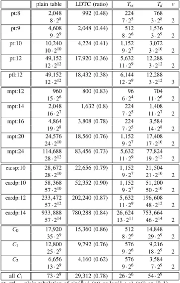
LDTC is now available in FloPoCo (git master branch), where it will benefit to all the table-based operators. Table III reports the compression rate in terms of bit count for a repre-sentative range of application (see section III). Compression ratio up to 0.36 are possible, to be be compared to the best ratio of 0.74 in the previous state of the art [7, Table VII].
A general observation on Table III is that the best com-pression ratios are observed for functions with the smaller difference between wR and wA. The intuition here is that the
larger table is always Td, and that Tdhas very few output bits
when wR≈ wA. Note that LDTC even works when wR< wA.
Looking at the pt results, the compression ratio seems to improve with the initial table size.
The optimal often has an overlap of v = 2 bits. As the ptl line shows, this is not a strict rule.
Table IV compares the cbitof the previous state of the art in multipartite methods [7, Tables 2 and 3] to that achieved by the multipartite implementation of FloPoCo when enhanced with LDTC. The function used here is sin(π
4x), the only one
on which we could reproduce the results of [7]. LDTC always improves upon MP, but not always over the hierarchical mul-tipartite method [7] which brings other improvements. There is one more addition in MP+LDTC than in HMP, however remark that the total number of bits input to the compressor tree is smaller for MP+LDTC (7+14+10+8+6+4=49, versus 20+12+10+8+6=56 for HMP) — both observations also hold in the 24-bit case, not detailed for space. Therefore the cost of the compressor tree is likely to be smaller for MP+LDTC.
TABLE III
COMPRESSION RESULTS IN TERMS OF BIT STORAGE
plain table LDTC (ratio) Tss Td v
pt:8 2,048 992 (0.48) 224 768 8 · 28 7 · 25 3 · 28 2 pt:9 4,608 2,048 (0.44) 512 1,536 9 · 29 8 · 26 3 · 29 2 pt:10 10,240 4,224 (0.41) 1,152 3,072 10 · 210 9 · 27 3 · 210 2 pt:12 49,152 17,920 (0.36) 5,632 12,288 12 · 212 11 · 29 3 · 212 2 ptl:12 49,152 18,432 (0.38) 6,144 12,288 12 · 212 12 · 29 3 · 212 3 mpt:12 960 800 (0.83) 96 704 15 · 26 6 · 24 11 · 26 2 mpt:14 2,048 1,632 (0.8) 224 1,408 16 · 27 7 · 25 11 · 27 2 mpt:16 4,864 3,808 (0.78) 224 3,584 19 · 28 7 · 25 14 · 28 2 mpt:20 24,576 18,560 (0.76) 1,152 17,408 24 · 210 9 · 27 17 · 210 2 mpt:24 114,688 83,456 (0.73) 5,632 77,824 28 · 212 11 · 29 19 · 212 2 ea:sp:10 28, 672 22,656 (0.79) 1, 152 21, 504 28 · 210 9 · 27 21 · 210 2 ea:dp:10 58, 368 52,352 (0.90) 1, 152 51, 200 57 · 210 9 · 27 50 · 210 2 ea:dp:12 233, 472 202,240 (0.87) 5, 632 196, 608 57 · 212 11 · 29 48 · 212 2 ea:dp:14 933, 888 780,288 (0.84) 26, 624 753, 664 57 · 214 13 · 211 46 · 214 2 C0 17,920 15,360 (0.86) 512 14,848 35 · 29 8 · 26 29 · 29 2 C1 12,800 9,792 (0.76) 576 9,216 25 · 29 9 · 26 18 · 29 2 C2 6,656 4,160 (0.62) 576 3,584 13 · 29 9 · 26 7 · 29 2 all Ci 73 · 29 29,312 (0.78) 26 · 26 54 · 29
pt, ptl plain tabulation of sin(π
4x) (pt) or log(1 + x) (ptl) on [0, 1)
mpt first table of a multipartite approximation [6] to sin(π
4x) on [0, 1)
ea eA table of [22], for single (sp) or double (dp) precision
Ci coefficients of a degree-2 uniform piecewise approximation [18]
to sin(π
4x) on [0, 1) for 32-bit accuracy (wA= 9)
TABLE IV
COMPARISON WITH THE STATE OF THE ART IN MULTIPARTITE METHODS
24 bits 16 bits
HMP [7] 166,528 6, 272 = 20 · 27+ 12 · 27+ 10 · 27+ 8 · 26+ 6 · 26
MP+LDTC 158,208 6, 752 = 7 · 25+ 14 · 28+ 10 · 27+ 8 · 27+ 6 · 26+ 4 · 26
TABLE V FPGAIMPLEMENTATION RESULTS FORsin(π
4x) (ADDITION INCLUDED)
case without LDTC with LDTC (ratio) pt:8 27 LUT 5.5 ns 26 LUT (0.96) 6.4 ns (1.17) pt:9 61 LUT 6.3 ns 46 LUT (0.75) 6.7 ns (1.08) pt:10 134 LUT 6.8 ns 83 LUT (0.62) 7.5 ns (1.1) pt:12 536 LUT 9.8 ns 287 LUT (0.54) 8.7 ns (0.89) mpt:12 76 LUT 7.6 ns 73 LUT (0.96) 7.7 ns (1.02) mpt:14 102 LUT 8.1 ns 98 LUT (0.96) 8.1 ns (1.0) mpt:16 184 LUT 8.9 ns 190 LUT (1.03) 9.3 ns (1.04) mpt:20 676 LUT 12.8 ns 637 LUT (0.94) 12.5 ns (0.98) mpt:24 2489 LUT 18.1 ns 2322 LUT (0.93) 16.1 ns (0.89) Results after implementation on Kintex7 using Vivado 2020.2. The
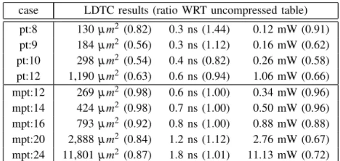
TABLE VI ASICIMPLEMENTATION RESULTS FORsin(π
4x) (ADDITION INCLUDED)
case LDTC results (ratio WRT uncompressed table) pt:8 130 µm2(0.82) 0.3 ns (1.44) 0.12 mW (0.91) pt:9 184 µm2(0.56) 0.3 ns (1.12) 0.16 mW (0.62) pt:10 298 µm2(0.54) 0.4 ns (0.82) 0.26 mW (0.58) pt:12 1,190 µm2(0.63) 0.6 ns (0.94) 1.06 mW (0.66) mpt:12 269 µm2(0.98) 0.6 ns (1.00) 0.34 mW (0.96) mpt:14 424 µm2(0.98) 0.7 ns (1.00) 0.50 mW (0.96) mpt:16 793 µm2(0.92) 0.8 ns (1.00) 0.88 mW (0.88) mpt:20 2,888 µm2(0.84) 1.2 ns (1.12) 2.76 mW (0.67) mpt:24 11,801 µm2(0.87) 1.8 ns (1.01) 11.13 mW (0.72)
Results obtained with Synopsys design compiler using STMicroelectronics 28nm FDSOI standard cell library. The compressor tree used for mpt is
FloPoCo’s default, which is currently optimized for FPGAs.
Results for FPGA and ASIC synthesis are reported in Tables V and VI respectively. All the LDTC were optimized using the cbit cost function, the other cost functions of Table II failing
to provide any significant improvement so far.
The area compression ratios in the synthesis results are not as good as those of Table III, and the difference cannot be explained by the addition cost only: the logic optimization of synthesis tools somehow discover some of the compression opportunity exploited by LDTC [17].
The compressed plain tables (pt lines in Table V) include an adder. Its area overhead is smaller than the area gained on the tables for precisions larger than 8 bits, however it adds to the critical path delay. Still, for large tables, LDTC also reduces the delay, both on ASIC and on FPGA.
In the multipartite cases (mpt lines in Table V), this addition is merged in the compressor tree (see Figure 4) and the delay is essentially unchanged in most cases, as expected2. However the area reduction is less dramatic as only one table out of several is compressed, and for some precisions LDTC may even be counter-productive area-wise.
We do not report results targetting FPGAs with block RAM. Actual savings will depend on the block RAM capabilities of the target, which are very discrete (e.g. M20k blocks on Altera/Intel devices can be configured as 29× 40, 210× 20,
or 211× 10 bits, while the Xilinx/AMD 36kbit blocks can do from 29× 72 to 215× 1). The larger the table, the higher the
chances that LDTC is useful.
VI. CONCLUSION
This work adds one optimization technique to the bag of tricks of arithmetic designers: lossless differential table com-pression can reduce up to a factor two the storage requirement of most tables used in function evaluation, at the cost of one small integer addition that can be hidden for free in an existing compressor tree. The optimal solution can be found by an exhaustive enumeration. This technique is available in the open-source FloPoCo core generator.
Acknowledgement: Many thanks to Fr´ed´eric P´etrot for his comments and his help with ASIC synthesis.
2The mpt timing variation in Table V are routing artifacts – even the
improvement for mpt:24 is actually due to variations in input buffer net delay.
REFERENCES
[1] J.-M. Muller, Elementary functions, algorithms and implementation, 3rd Edition. Birkha¨user Boston, 2016. [Online]. Available: https://hal-ens-lyon.archives-ouvertes.fr/ensl-01398294
[2] A. Omondi, Computer-Hardware Evaluation of Mathematical Functions. Imperial College Press, 2016.
[3] F. de Dinechin and A. Tisserand, “Multipartite table methods,” IEEE Transactions on Computers, vol. 54, no. 3, pp. 319–330, 2005. [4] J. Detrey and F. de Dinechin, “Table-based polynomials for fast hardware
function evaluation,” in Application-specific Systems, Architectures and Processors. IEEE, 2005, pp. 328–333.
[5] D.-U. Lee, P. Cheung, W. Luk, and J. Villasenor, “Hierarchical segmen-tation schemes for function evaluation,” IEEE Transactions on VLSI Systems, vol. 17, no. 1, 2009.
[6] S.-F. Hsiao, P.-H. Wu, C.-S. Wen, and P. K. Meher, “Table size reduction methods for faithfully rounded lookup-table-based multiplierless func-tion evaluafunc-tion,” Transacfunc-tions on Circuits and Systems II, vol. 62, no. 5, pp. 466–470, 2015.
[7] S.-F. Hsiao, C.-S. Wen, Y.-H. Chen, and K.-C. Huang, “Hierarchical multipartite function evaluation,” Transactions on Computers, vol. 66, no. 1, pp. 89–99, 2017.
[8] D. De Caro, E. Napoli, D. Esposito, G. Castellano, N. Petra, and A. G. Strollo, “Minimizing coefficients wordlength for piecewise-polynomial hardware function evaluation with exact or faithful rounding,” IEEE Transactions on Circuits and Systems I: Regular Papers, vol. 64, no. 5, pp. 1187–1200, 2017.
[9] K. Chapman, “Fast integer multipliers fit in FPGAs (EDN 1993 design idea winner),” EDN magazine, no. 10, p. 80, May 1993.
[10] M. Wirthlin, “Constant coefficient multiplication using look-up tables,” Journal of VLSI Signal Processing, vol. 36, no. 1, pp. 7–15, 2004. [11] F. de Dinechin, S.-I. Filip, L. Forget, and M. Kumm, “Table-based versus
shift-and-add constant multipliers for FPGAs,” in 26th IEEE Symposium of Computer Arithmetic (ARITH-26), Jun. 2019.
[12] F. de Dinechin, M. Istoan, and G. Sergent, “Fixed-point trigonometric functions on FPGAs,” SIGARCH Computer Architecture News, vol. 41, no. 5, pp. 83–88, 2013.
[13] E. E. Swartzlander, “Merged arithmetic,” IEEE Transactions onComput-ers, vol. C-29, no. 10, pp. 946 –950, 1980.
[14] H. Parendeh-Afshar, A. Neogy, P. Brisk, and P. Ienne, “Compressor tree synthesis on commercial high-performance FPGAs,” ACM Transactions on Reconfigurable Technology and Systems, vol. 4, no. 4, 2011. [15] M. Kumm and J. Kappauf, “Advanced compressor tree synthesis for
FPGAs,” IEEE Transactions on Computers, vol. 67, no. 8, pp. 1078– 1091, 2018.
[16] N. Brisebarre and S. Chevillard, “Efficient polynomial L∞-
approxima-tions,” in 18th Symposium on Computer Arithmetic. IEEE, 2007, pp. 169–176.
[17] O. Gustafsson and K. Johansson, “An empirical study on standard cell synthesis of elementary function lookup tables,” Asilomar Conference on Signals, Systems and Computers, pp. 1810–1813, 2008.
[18] F. de Dinechin, M. Joldes, and B. Pasca, “Automatic generation of polynomial-based hardware architectures for function evaluation,” in Application-specific Systems, Architectures and Processors. IEEE, 2010.
[19] S.-F. Hsiao, H.-J. Ko, and C.-S. Wen, “Two-level hardware function evaluation based on correction of normalized piecewise difference func-tions,” IEEE Transactions on Circuits and Systems II: Express Briefs, vol. 59, no. 5, pp. 292–296, 2012.
[20] D. Chen and S.-B. Ko, “A dynamic non-uniform segmentation method for first-order polynomial function evaluation,” Microprocessors and Microsystems, vol. 36, pp. 324–332, 2012.
[21] P. T. P. Tang, “Table-driven implementation of the exponential function in IEEE floating-point arithmetic,” ACM Transactions on Mathematical Software, vol. 15, no. 2, pp. 144–157, 1989.
[22] F. de Dinechin and B. Pasca, “Floating-point exponential functions for DSP-enabled FPGAs,” in Field Programmable Technologies, Dec. 2010, pp. 110–117.
[23] M. Langhammer and B. Pasca, “Single precision logarithm and ex-ponential architectures for hard floating-point enabled FPGAs,” IEEE Transactions on Computers, vol. 66, no. 12, pp. 2031–2043, 2017. [24] J.-A. Pi˜neiro, M. Ercegovac, and J. Bruguera, “High-radix logarithm
with selection by rounding: Algorithm and implementation,” Journal of VLSI signal processing systems for signal, image and video technology, vol. 40, no. 1, pp. 109–123, 2005.
[25] M. D. Ercegovac and T. Lang, Digital Arithmetic. Morgan Kaufmann, 2004.
![Fig. 2. A fixed-point polynomial evaluator, using uniform segmentation and a Horner scheme with truncated multipliers – see [18] for more details.](https://thumb-eu.123doks.com/thumbv2/123doknet/14233125.485803/4.918.477.835.257.373/polynomial-evaluator-uniform-segmentation-horner-truncated-multipliers-details.webp)