Dual Coordinate Ascent Methods for
Linear Network Flow Problems*
by
Dimitri P. Bertsekas and Jonathan Eckstein Laboratory for Information and Decision Systems
and Operations Research Center Massachusetts Institute of Technology
Cambridge, Mass. 02139
Abstract
We review a class of recently-proposed linear-cost network flow methods which are amenable to parallel implementation. All the methods in the class use the notion of c-complementary slackness,
and most do not explicitly manipulate any "global" objects such as paths, trees, or cuts. Interestingly, these methods have also stimulated a large number of new serial computational complexity results. We develop the basic theory of these methods and present two specific
methods, the E-relaxation algorithm for the minimum-cost flow problem, and the auction algorithm for assignment problem. We show how to implement these methods with serial complexities of
O(N3 log NC) and O(NA log NC), respectively. We also discuss practical implementation issues and computational experience to date. Finally, we show how to implement e-relaxation in a completely asynchronous, "chaotic" environment in which some processors compute faster than others, some processors communicate faster than others, and there can be arbitrarily large communication delays.
Key Words: Network flows; relaxation; distributed algorithms; complexity; asynchronous algorithms.
* Supported by Grant NSF-ECS-8217668 and by the Army Research Office under grant DAAL03-86-K-0171. Thanks are due to Paul Tseng and Jim Orlin for their helpful comments.
1.
Introduction
This paper considers a number of recent developments in network optimization, all of which originated from efforts to construct parallel or distributed algorithms. One obvious idea is to have a processor (or virtual processor) assigned to each node of the problem network. The intricacies of coordinating such processors makes it awkward to manipulate the "global" objects - such as cuts, trees, and augmenting paths - that are found in most traditional network algorithms. As a
consequence, algorithms designed for such distributed environments tend to use only local
information: the dual variables associated with a node and its neighbors, and the flows on the arcs incident to the node. For reasons that will become apparent later, we call this class of methods dual coordinate ascent methods. Their appearance has also stimulated a flurry of advances in serial computational complexity results for network optimization problems.
Another feature of this class of algorithms is that they all use a notion called e-complementary slackness. As we shall see, this idea is essential to making sure that a method that uses only local information does not "jam" or halt at a suboptimal point. However, e-complementary slackness is also useful in the construction of scaling algorithms. The combination of scaling and
e-complementary slackness has given rise to a number of computational complexity results, most of them serial. Some of the algorithms behind these results use only local information, but others use
global data, usually to construct augmenting paths.
In this paper, we will concentrate on local algorithms, since they are the ones which hold the promise of efficient parallel implementation, and show how they can be regarded as coordinate
ascent or relaxation methods in an appropriately-formulated dual problem. We will then take a detailed look at what is perhaps the generic algorithm of the class, the e-relaxation algorithm, and
give both scaled and unscaled complexity results for it. We will also consider a related algorithm for assignment problems, which we call auction, along with its scaled and unscaled complexities. We discuss the practical performance of these algorithms, based on preliminary experimentation.
Finally, we will present an implementation of e-relaxation that works in a completely asynchronous, chaotic environment.
2.
Basic Concepts
2.1. DualityWe first introduce the minimum-cost flow problem and its dual. Consider a directed graph with node set N and arc set A, with each arc (i, j) having a cost coefficient aij. Letting fij be the flow of the arc (i, j), the classical min-cost flow problem ([36], Ch.7) may be written
minimize X(ij)eA aijfij (MCF)
subject to
Z(i,j)eA fij - C(j,i)eA fji = Si V i E N (1)
bij < fij < cij ~V (i, j) E A, (2)
where aij, bij, ci, and si, are given integers. In order for the constraints (1) to be consistent, we require that liEN Si = 0. We also assume that there exists at most one arc in each direction
between any pair of nodes, but this assumption is for notational convenience and can be easily dispensed with. We denote the numbers of nodes and arcs by N and A, respectively. Also, let C denote the maximum absolute value of the cost coefficients, max(i, j)e A laijl.
In this paper, aflow f will be any vector in RA, with elements denoted fij, (i, j) E A. A
capacity-feasible flow is one obeying the capacity constraints (2). If a capacity-feasible flow also obeys the conservation constraints (1), it is afeasible flow.
We formulate a dual problem to (MCF) by associating a Lagrange multiplier Pi with each conservation of flow constraint (1). Letting f be a flow and p be the vector with elements Pi, i e N, we can write the corresponding Lagrangian function as
L(f, p) = ](i,j)EA (aij + Pj - Pi) fij + XiEN SiPi (3)
One obtains the dual function value q(p) at a vector p by minimizing L(f, p) over all capacity-feasible flows f. This leads to the dual problem
maximize q(p) (4)
subject to no constraint on p, with the dual functional q given by
= (i,j)EA qij(Pi - Pj) + lieN SiPi (5a) where
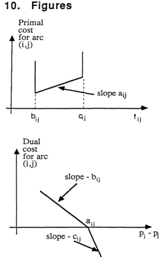
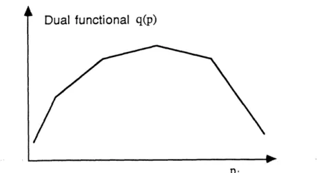
qij(Pi - pj) = min fij {(aij + Pj - Pi)fij I bij < fij < cij } (5b) The function qij is shown in Figure 1. This formulation of the dual problem is consistent with conjugate duality frameworks [39], [40] but can also be obtained via linear programming duality theory [32], [36]. We henceforth refer to (MCF) as the primal problem, and note that standard duality results imply that the optimal primal cost equals the optimal dual cost. We refer to the dual variable Pi as the price of node i.
The results of this paper admit extension to the case where some or all of the cij are infinite, introducing constraints into the dual problem. We omit these extensions in the interest of brevity.
2.2. Primal-Dual Coordinate Ascent: the Up and Down Iterations
We have now obtained a dual problem which is piecewise-linear and unconstrained. A straightforward approach to distributed unconstrained optimization is to have one processor
responsible for maximization along each coordinate direction. However, the nondifferentiability of the dual function q presents special difficulties.
Because of these difficulties, the algorithms we will examine in this paper are in fact primal-dual methods, in that they maintain not only a vector of prices p, but also a capacity-feasible flow f such that f and p jointly satisfy (perhaps approximately) the complementary slackness conditions
fij <cij Pi- Pj < aij V(i, j) e A (6a)
bij < fij Pi- Pj > aij V (i,j) E A . (6b)
Standard linear programming duality theory gives that f and p are jointly optimal for the primal and dual problems, respectively, if and only if they satisfy complementary slackness and f is feasible.
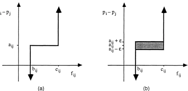
Appealing to conjugate duality theory ([39] and [40]), there is a useful interpretation of the complementary slackness conditions (6a-b). Referring to Figure 1, the complementary slackness conditions on (i, j) and the capacity constraint bij < fij < cij are precisely equivalent to requiring that -fij be a supergradient of the dual function component qij at the point Pi-Pj. This may be written -fij E aqij(pi-pj). Adding these conditions together for all arcs incident to a given node i and using the definition of the dual functional (5a), one obtains that the surplus of node i, defined to be
is in fact a supergradient of q(p) considered as a function of Pi, with all other node prices held constant. We may express this as gi E
aqi(Pi;
p), where qi( ; p) denotes the function of a single variable obtained from q by holding all prices except the ith fixed at p. The surplus also has theobvious interpretation as the flow into node i minus the flow out of i given by the (possibly infeasible) flow f. Thus a flow f is feasible if and only if the corresponding surpluses gi are zero for all iE N. (Note that the sum of all the surpluses is zero for any flow.)
We make a few further definitions: we say that an arc (i, j) is
Inactive if Pi < aij + Pj (8a)
Balanced if Pi = aij + Pj (8b)
Active if Pi > aij +Pj . (8c)
The combined condition -fij e aqij(pi-pj) may then be reexpressed as
fij = bij, if (i, j) active (9a)
bij <fij < cij, if (i, j) balanced (9b)
fij = cij, if (i, j) active . (9c)
Figure 2 displays the form of the dual function along a single price coordinate Pi. The breakpoints along the curve correspond to points where one or more arcs incident to node i are balanced. Only at the breakpoints is there any freedom in choosing arc flows; on the linear portions of the graph, all arcs are either active or inactive, and all flows are determined exactly by (9a) and (9c).
It is now clear how to maintain a pair (f, p) satisfying complementary slackness while altering a single dual variable Pi. Each time Pi passes through a breakpoint, one simply sets each arc incident to i to its upper flow bound if it has become active, or to its lower flow bound if it has become inactive. Often, however, it is useful to perform a somewhat more involved calculation that takes advantage of the supergradient properties of the surplus gi. This calculation also supplants any direct computation the directional derivatives of q. Suppose that we have (f, p) satisfying complementary slackness, some node i for which gi > 0, and we are at a breakpoint in the dual cost. Since gi is a supergradient of qi(pi; p), decreasing Pi must decrease the dual objective value q, so either the current value of Pi is optimal or it should be increased. We then try to decrease the surplus gi of i by "pushing" flow on the balanced arcs incident to i - that is, increasing the flow on balanced outgoing arcs and decreasing the flow on incoming balanced arcs, to the extent permitted by the capacity constraints (2). If the surplus can be reduced to zero in this way, we conclude that Oe aqi(Pi; p), and hence that the current value of Pi is optimal. Otherwise, we set all outgoing balanced arcs to their maximum flow, and all incoming balanced arcs to their minimum. The resulting surplus gi is then the minimal member of aqi(pi; p), and hence (by the concavity of
q) the directional derivative of q in the positive Pi direction. Consequently, we may improve the dual objective by increasing Pi until we reach the next breakpoint, that is, until another arc becomes balanced. At this point, we repeat the entire procedure, stopping only when we obtain gi = 0.
What we have just described is the basic outline of what we call the up iteration, which is central to all dual coordinate ascent methods. It maximizes q along the Pi coordinate by increasing Pi, while maintaining the capacity constraints and the complementary slackness of f and p. It reduces the surplus of the node i to zero. There is also an entirely analogous down iteration that applies to nodes with gi < 0, reduces the variable Pi, and increase gi to zero.
2.3. Jamming and the RELAX Approach
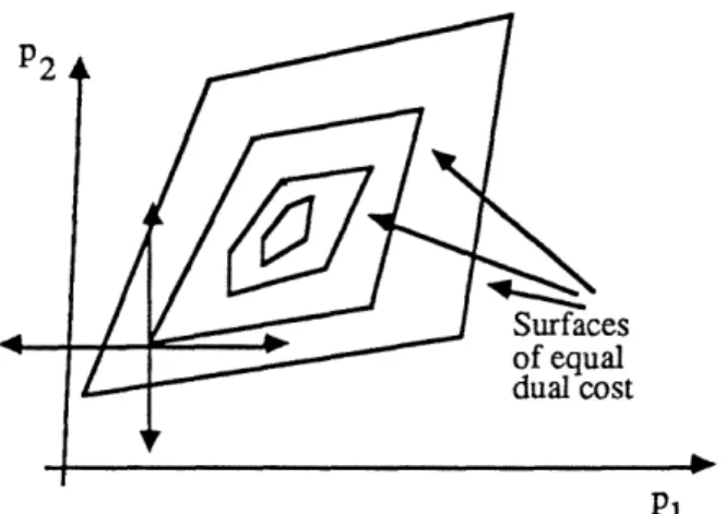
At this point, it may seem appealing to consider maximizing the dual function by starting with some arbitrary pair (f, p) satisfying (9a-c) and repeatedly applying up and down iterations until all nodes have zero surplus. It would then follow that the final f and p obtained would be primal and dual optimal, respectively. Unfortunately, as shown in Figure 3, a nondifferentiable function such as q, although continuous and concave, may have suboptimal points where it cannot be improved by either increasing or decreasing any single variable. If this naive algorithm were to encounter such a point, it would perform an infinite sequence of changes to the flow fij without ever halting or changing the dual prices p. We call this phenomenon jamming.
One way of avoiding the jamming problem is embodied in the RELAX family of serial
computer codes (see [11], [13], [43]). Essentially, these codes make dual ascents along directions that have a minimal number of non-zero components, which means that they select coordinate directions whenever possible. Only when jamming occurs do they select more complicated ascent directions. These codes have proved remarkably efficient in practice; however, they are not particularly suitable for massively parallel environments because of the difficulties of coordinating
simultaneous multiple-node price change and labelling operations.
Note that jamming would not occur if the dual cost were differentiable. If the primal cost function is strictly convex, then the dual cost is indeed differentiable, and application of coordinate
ascent is straightforward and well-suited to parallel implementation. Proposals for methods of this type include [41], [19], [35], [21], and [33]. [45] contains computational results on a simulated parallel architecture, and [44] results on an actual parallel machine. [14] and [15] contain
2.4. The Auction Approach
A different, more radical approach to the jamming problem is to allow small price changes, say by some amount £, even if they worsen the dual cost. This idea dates back to the auction algorithm ([8],[9],[10]), a procedure for the assignment (bipartite matching) problem that actually predates the RELAX family of algorithms. In this algorithm, one considers the nodes on one side of the bipartite graph to be "people" or agents placing bids for the "objects" represented the nodes on the other side of the graph. The dual variables pj co:responding to the "object" nodes may then be considered to be the actual current prices of the objects in the auction. The phenomenon of jamming in this context manifests itself as two or more people submitting the same bid for an
object. In a real auction, such conflicts are resolved by people submitting slightly higher bids, thus raising the price of the object, until all but one bidder drops out and the conflict is resolved (we give a more rigorous description of the auction algorithm later in this paper).
This idea of resolving jamming by forcing (small) price increases even if they worsen the dual cost is also fundamental to the central algorithm of this paper, which we call c-relaxation. First, we must introduce the concept of E-complementary slackness.
2.5. e-Complementary Slackness
The e-complementary slackness conditions are obtained by "softening" the two inequalities of the conventional complementary slackness conditions (6a-b) by an amount £ 2 0, yielding:
fi < cij Pi - Pj < aij + £ (10a)
bij < fij ~ Pi - pj 2 aij - £ . (10b)
The "kilter diagrams" of Figure 4 display the relationship imposed between Pi - pj and fij by both e-complementary slackness and regular complementary slackness. We say that the arc (i, j) is
e-Inactive if Pi < aij +Pj- (1la)
E--Balanced if pi = aij +Pj - ( lb)
E-Balanced if aij + pj - £ < Pi < aij + pj +£ (11c)
£+-Balanced if Pi = aij + Pj p + (1 ld)
e-Active if Pi > aij ++ £ (1 le)
Note that e--balanced and £+-balanced are both special cases of e-balanced The e-complementary slackness conditions (combined with the arc capacity conditions) may now also be expressed as
fij = bij if (i, j) is e-inactive (12a)
fij = cij if (i, j) is c-active . (12c) The usefulness of £-complementary slackness is evident in the following proposition:
Proposition 1: If £ < 1/N, f is primal feasible (it meets both constraints (1) and (2)), and f and p jointly satisfy c-CS, then f is optimal for (MCF).
Proof: If f is not optimal then there must exist a simple directed cycle along which flow can be increased while the primal cost is improved. Let Y+ and Y- denote the sets of arcs of forward and backward arcs in the cycle, respectively. Then we must have
(i,j)Ey+ aij - (ij)Y- aij < 0 (13a)
fi < cij for (i, j)e Y+ (13b)
bij < fij for (i,j) E Y-. (13c)
Using (10a-b), we have
Pi < pj + aij + £ for (i,j) e Y+ (14a)
Pj < Pi- aij +£ for (i,j) e Y-. (14b)
Adding all the inequalities (14a) and (14b) together and using the hypothesis e < 1/N yields (ij) y+ aij - (ij) Y- aij > - Ne > -1
Since the aij are integral, this contradicts (13a). QED.
A strengthened form of Proposition 1 also holds when the arc cost coefficients and flow bounds are not integer, and is obtained by replacing the condition e<1/N with the condition
£ < A min I of arc Length Lengthof Y < 0 (15)
All directed cycles Y Number of arcs in Y
where
Length of cycle Y = yi(ij)EY+ aij - J(ij)e y- aij (16)
The proof is obtained by suitably modifying the last relation in the proof of Proposition 1. A very useful special case is that f is optimal if e < d/N, where d is the greatest common divisor of all the arc costs. When all arc costs are integer, we are assured that d > 1.
The notion of e-complementary slackness was used in [8], [9], and introduced more formally in [13], [14]. It was also used in the analysis of [42] (Lemma 2.2) in the special case where the flow vector f is feasible. A useful way to think about e-complementary slackness is that if the pair (f, p) obey it, then the rate of decrease in the primal cost to be obtained by moving flow around a directed
cycle Y without violating the capacity constraints is at most IYle. It limits the steepness of descent along the elementary directions (using the terminology of [39]) of the primal space.
2.6. The Basics of the e-Relaxation Method
We are now ready to describe the outlines of the e-relaxation algorithm. It starts with any integer flow f and prices p satisfying e-complementary slackness. Such a pair may be constructed by choosing p arbitrarily and then constructing f so as to obey (12a-c). The algorithm then
repeatedly selects nodes i with positive surplus (gi > 0) and performs up iterations at them. Unlike the basic up iteration described above, though, these iterations set Pi to a value e above the
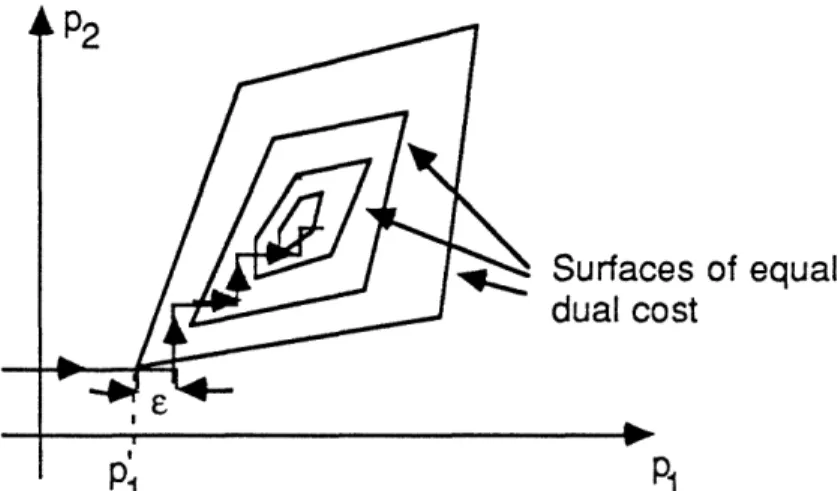
maximizer of the dual cost with respect to Pi. The flow is adjusted to maintain integrality and e-complementary slackness, but not necessarily regular e-complementary slackness. As we shall prove below, this process will eventually drive all the nodes' surpluses to zero, resulting in a pair (f, p) satisfying the conditions of Proposition 1 (presuming e < 1/N). It avoids jamming by following paths such as those depicted in figure 5. If e > d/N, where d is the greatest common divisor of the arc costs, the algorithm will still terminate with a feasible flow, but this flow may not be optimal.
2.7. The Goldberg-Tarjan Maximum Flow Method
Another important algorithm belonging to the dual coordinate ascent class is the maximum flow method of Goldberg and Tarjan ([26] and [27]). This algorithm was developed roughly
concurrently with, and entirely independently from, the RELAX family of codes. The original motivation for this algorithm seems to have been quite different than the theory we have developed above; it appears to have been originally conceived of as a distributed, approximate computation of the "layered" representation of the residual network that is common in maximum flow algorithms
[23]. However, it turns out that the first phase of this two-phase algorithm, in its simpler implementations, is virtually identical to e-relaxation as applied to a specific formulation the maximum flow problem. This connection will become apparent later. Basically, the distance estimates of the maximum flow algorithm may be interpreted as dual variables, and the method in fact maintains e-complementary slackness with e=1.
The connection between the Goldberg-Tarjan maximum flow and c-relaxation provided two major benefits: e-relaxation gives a natural, straightforward way of reducing the maximum flow method to a single phase, and much of the maximum flow method's complexity analysis could be applied to the case of e-relaxation.
2.8. Complexity Analysis
There are several difficulties in adapting the maximum flow analysis of [26] and [27] to the case of c-relaxation. The first is in placing a limit on the amount that prices can rise. The approach taken here synthesizes the ideas of [7] with those of [28]-[30]. This methodology can also be applied directly to solving maximum flow problems with arbitrary initial prices.
Another problem is that offlow looping. This is discussed in Section 4.4 (see figure 7), and refers to a phenomenon whereby small increments of flow move an exponential number of times around a loop without any intermediate price changes. To overcome this difficulty one must initialize the algorithm in a way that the subgraph of arcs along which flow can change is acyclic at all times. In the max-flow problem this subgraph is naturally acyclic, so this difficulty does not arise. Flow looping is also absent from the assignment problem because all arcs may be given a capacity of 1, and (as we shall see) the algorithm changes flows by integer amounts only.
Section 4.4 also discusses the problem of relaxing nodes out of order. The acyclic subgraph mentioned above defines a partial order among nodes, and it is helpful to operate on nodes
according to this order. This idea is central in the complexity analysis of [7], and leads to a simple and practical implementation that maintains the partial order in a linked list. We call this the sweep
implementation. This analysis, essentially given in [7], provides an O(N23/£) complexity bound
where
3
is a parameter bounded by the maximum simple path length in the network where the length of arc (i, j) is laijl. Maximum flow problems can be formulated so that 3/£=O(N), giving an O(N3) complexity bound for essentially arbitrary initial prices. For other minimum cost flow problems, including the assignment problem, the complexity is pseudopolynomial, being sensitive to the arc cost coefficients. The difficulty is due to a phenomenon which we call price haggling. This is analogous to the ill-conditioning phenomenon in unconstrained optimization, and ischaracterized by an interaction in which several nodes restrict one another from making large price changes (see section 6 and 7.1). This paper emphasizes degenerate price rises, which are critical to overcoming price haggling, and shows that they can be implemented in a way that does not alter the e-relaxation method's theoretical complexity.
2.9. Developments in Scaling
e-complementary slackness is also useful in constructing scaling algorithms, which conversely help to overcome the problem of price haggling. We first distinguish between two kinds of
scaling: cost scaling and e-scaling. In cost scaling algorithms (which have their roots in [23]), one holds e fixed and gradually introduces more and more accurate cost data; in e-scaling, the cost data
may be greater than or equal to d/N. Computational experiments on e-scaling in the auction algorithm were done in 1979 [8] and again in 1985 [9]. The method of c-scaling was first analyzed in [28], where an algorithm with O(NAlog(N)log(NC)) complexity was proposed, and a contrast with the method of cost scaling was drawn. The complexity of this algorithm was fully established in [29] and [30], where algorithms with O(N5/3A2/31og(NC)) and O(N31og NC) complexity were also given, and parallel versions were also discussed. The first two algorithms use complex, sophisticated data structures, while the O(N31og(NC)) algorithm makes use of the sweep implementation. Both also employ a variation of e-relaxation we call broadbanding, which will be described later in this paper. Independent discovery of the sweep implementation (there called the wave implementation) is claimed in [30]. These results improved on the complexity bounds of all alternative algorithms for (MCF), which in addition are not as well suited for parallel implementation as the e-relaxation method. Scaling analyses similar to [28] appeared later in such works as [24], [25], and [2].
In this paper we show how to moderate the effect of price haggling by using a similar but more traditional cost scaling approach in place of e-scaling. This, in conjunction with the sweep
implementation, leads to a simple algorithm with an O(N31ogNC) complexity. This approach also bypasses the need for the broadbanding modification to the basic form of the e-relaxation method, introduced in [28]-[30] in conjunction with e-scaling.
Usually the most challenging part of scaling analysis ([18], [23], [28]-[30], [34], [38], [42]) is to show how the solution of one subproblem can be used to obtain the solution of the next
subproblem relatively quickly. Here, the main fact is that the final price-flow pair (p, f) of one subproblem violates the e-CS conditions for the next one by only a small amount. A way of taking advantage of this was first proposed in Lemmas 2-5 of [28] (see also [29], [30]). A key lemma is Lemma 5 of [28], which shows that the number of price changes per node needed to obtain a
solution of the next subproblem is O(N). There is a similar lemma in [18] that bounds the number of maximum flow computations in a scaling step in an O(N4logC) algorithm based on the primal-dual method. Our Lemma 5 of this paper is a refinement of Lemma 5 of [28], but is also an extension of Corollary 3.1 of [7]. We introduce a measure 3(pO) of suboptimality of the initial price vector pO, whereas [28]-[30] use an upper bound on this measure. This extension allows the lemma to be used in contexts other than scaling.
3.
The £-Relaxation Method in Detail
To discuss e-relaxation in detail, we must first be more specific about when the method is actually allowed to change the flow along an arc.
3.1. The Admissible Graph
When the e-relaxation algorithm is performing an up iteration at some node i, it only performs two kinds of flow alterations: flow increases on outgoing e+-balanced arcs (i, j) with fij < cij, and flow decreases on incoming e--balanced arcs (j, i) with fji > bji. We call these two kinds of arcs admissible. The admissible graph G* corresponding to a pair (f, p) is the directed (multi)graph with node set N, an edge (i, j) for each e+-balanced arc (i, j) in A with fij < cij, and a reverse edge (j, i) for each e--balanced arc (i, j) in A with fij > bij. It is similar to the residual graph
corresponding to the flow f which has been used by many other authors (see [36], for example), but only contains edges corresponding to arcs that are admissible.
3.2. Push Lists
To obtain an efficient implementation of c-relaxation, one must store a representation of the admissible graph. We use a simple "forward star" scheme in which each node i stores a linked list containing all the arcs corresponding to edges of the admissible graph outgoing from i - that is, all arcs whose flow can be changed by iterations at i without any alteration in p. We call this list a push list. Although it is possible to maintain all push lists exactly at all times, doing so requires
manipulating unnecessary pointers; it is more efficient to allow some inadmissible arcs to creep onto the push lists. However, all push lists must be complete: that is, though it may contain some extra arcs, i's push list must contain every arc whose flow can be altered by iterations at i without a price change.
The complexity results in most of the earlier work on the dual coordinate ascent class of algorithms ([26],[27],[28],[7]) implicitly require push lists or something similar. The first time push lists seem to have been discussed explicitly is in [30], where they are called edge lists.
3.3. The Exact form of the Up Iteration
Assume that f is a capacity-feasible flow, the pair (f, p) obeys E-complementary slackness, a push list corresponding to (f, p) exists at each node, and all these lists are complete. Let ie N be a node with positive surplus (gi > 0).
Up Iteration:
Step 1: (Find Admissible Arc) Remove arcs from the top of i's push list until finding one which is still admissible (this arc is not deleted from the list). If gi > 0 and the arc so found is an outgoing arc (i, j), go to step 2. If gi > 0 and the arc found is an incoming arc (j, i), go to step 3. If the push list has become empty, go to Step 4. If an arc was found but gi= 0, stop.
Step 2: (Decrease surplus by increasing fij) Set
fij := fij + 6 gi := gi -gj := -gj + ,
where 5 = min{gi, cij - fij}. If 6 = cij - fij, delete (i, j) from the i's push list (it must be the top item). Go to step 1.
Step 3: (Decrease surplus by reducing fji) Set
fji:= fji- a
gi := gi - 6 gj := gj + ,
where 6 = min{gi, fji - bji}. If 6 = fji - bji, delete (i, j) from the i's push list (it must be the top item). Go to step 1.
Step 4: (Scan/Price Increase) By scanning all arcs incident to i, set
pi :=min{{pj + aij+e [ (i,j) E A andfij < cij} u
{pj - aji + (j, i) E A and bji < fji}} (17) and construct a new push list for i, containing exactly those incident arcs which are admissible with the new value of Pi. Go to Step 1. (Note: If the set over which the minimum in (17) is taken is empty and gi > 0, halt with the conclusion that the problem is infeasible - see the comments below. If this set is empty and gi = 0, increase Pi by £ and stop.)
The serial e-relaxation algorithm consists of repeatedly selecting nodes i with gi > 0, and
performing up iterations at them. The method terminates when gi < 0 for all iE N, in which case it follows that gi = 0 for all ie N, and that f is feasible.
3.4. Basic Lemmas
To see that execution of step 4 must lead to a price increase note that when it is entered, fij = cij for all (i, j) such that Pi > Pj + aij + e (18a) bji = fji for all (j, i) such that Pi >pj - aji + e, (18b) which may be obtained by combining that the push list is empty and complete with e-complementary slackness. Therefore, when Step 4 is entered we have
Pi < min{pj + aij + e
I
(i, j) E A and f ij < cij} (19a) Pi < min{pj - aji + e [ (j, i) E A and bji < fji} . (19b)It follows that step (4) must increase Pi, unless gi > 0 the set over which the minimum is taken is empty. In that case, fij = cij for all (i, j) outgoing from i and bji = fji for all (j, i) incoming to i, so the maximum possible flow is going out of i while the minimum possible is coming in. If gi > 0 under these circumstances, then the problem instance must be infeasible.
Lemma 1. The e-relaxation algorithm preserves the integrality of f, the e-complementary slackness conditions, and the completeness of all push lists at all times. All node prices are monotonically nondecreasing throughout the algorithm.
Proof: By induction on the number of up iterations. Assume that all the conditions hold at the outset of an iteration at node i. From the form of the up iteration, all changes to f are by integer amounts and 8-complementary slackness is preserved. By the above discussion, the iteration can only raise the price of i. Only inadmissible arcs are removed from i's push list in steps 1, 2, and 3, and none of these steps change any prices; therefore, steps 1, 2, and 3 preserve the completeness of push lists. In step 4, i's push list is constructed exactly, so that push list remains complete. Finally, we must show that the price rise at i does not create any new admissible arcs that should be on other nodes' push lists. First, suppose (j, i)e A becomes e+-balanced as a result of a price rise at i. Then (j, i) must have been formerly e-active, hence fji =cji, and (i, i) cannot be
admissible. A similar argument applies to any (i, j) that becomes 8--balanced as a result of a price rise at i. We have thus shown that all edges added to the admissible graph by step 4 are outgoing
from i. QED.
Lemma 2. Suppose that the initial prices Pi and the arc cost coefficients aij are all integer multiples of e. Then every execution of step 4 results in a price rise of at least e, and all prices remain multiples of e throughout the 8-relaxation algorithm.
Proof: It is clear from the form of the up iteration that it preserves the divisibility of all prices by
execution of step 4 results in a price increase. The lemma follows by induction on the number of up iterations. QED.
We henceforth assume that all arc costs and initial prices are integer multiples of £. A
straightforward way to do this, considering the standing assumption that the aij are integer, is to let
£ = l/k, where k is a positive integer, and assume that all Pi are multiples of 1/k. If we wish to satisfy the conditions of proposition 1, a natural choice for k is N+1.
Lemma 3. An up iteration at node i can only increase the surplus of nodes other than i. Once a node has nonnegative surplus, it continues do so for the rest of the algorithm. Nodes with negative surplus have the same price as they did at the outset of the algorithm.
Proof: The first statement is a direct consequence of the statement of steps 2 and 3 of the up iteration. The second then follows because each up iteration cannot drive the surplus of node i below zero, and can only increase the surplus of adjacent nodes. For the same reasons, a node with negative surplus can never have been the subject of an up iteration, and so its price must be the same as at initialization, proving the third claim. QED.
3.5. Finiteness
We now prove that the £-relaxation algorithm terminates finitely. Since we will be giving an exact complexity estimate in the next section, this proof is not strictly necessary. However, it serves to illuminate the workings of the algorithm without getting involved in excessive detail. Proposition 2: If problem (MCF) is feasible, the pure form of the e-relaxation method terminates with (f, p) satisfying e-CS, and with f being integer and primal feasible.
Proof: Because prices are nondecreasing (lemma 1), there are two possibilities: either (a) the prices of a nonempty subset N°°of N diverge to +oo, or else (b) the prices of all nodes in N remain bounded from above.
Suppose that case (a) holds. Then the algorithm never terminates, implying that at all times there must exist a node with negative surplus which, by lemma 3, must have a constant price. Thus, N-is a strict subset of N. To preserve e-CS, we must have after a sufficient number of iterations
fij = cij for all (i, j) E A with i e N°°, j X N° (20a) fji = bji for all (j, i) e A with i E N° , j X No (20b) while the sum of surpluses of the nodes in No is positive. This means that even with as much flow as arc capacities allow coming out of N° to nodes j X N-° , and as little flow as arc capacities allow coming into N°° from nodes j o N°°, the total surplus I{gi I i E N°°} of nodes in N°°is
positive. It follows that there is no feasible flow vector, contradicting the hypothesis. Therefore case (b) holds, and all the node prices stay bounded.
We now show that the algorithm terminates. If that were not so, then there must exist a node i E N at which an infinite number of iterations are executed. There must also exist an adjacent £--balanced arc (j, i), or £+-£--balanced arc (i, j) whose flow is decreased or increased (respectively) by an integer amount during an infinite number of iterations. For this to happen, the flow of (j, i) or (i, j) must be increased or decreased (respectively) an infinite number of times due to iterations at the adjacent node j. This implies that the arc (j, i) or (i, j) must become £+-balanced or e--balanced from e-balanced or £+-balanced (respectively) an infinite number of times. For this to happen, the price of the adjacent node j must be increased by at least 2e an infinite number of times. It follows that pj--o which contradicts the boundedness of all node prices shown earlier. Therefore the algorithm must terminate. QED.
3.6. Variations
3.6.1. Degenerate Price Rises
Note that when the push list is empty, the price Pi of the current node will be raised at the end of an up iteration even when gi = 0. We call such a price rise degenerate. Such price rises can be viewed as optional, and do not affect the finiteness or complexity of the algorithm. It is possible to
omit them completely, and halt the up iteration as soon as gi = 0. However, our computational experience has shown that degenerate price rises are a very good idea in practice. Similar price changes are very useful in the RELAX family of algorithms.
Following the analysis of directional derivatives and supergradients of section 2.3, one may show that at the end of the iteration, Pi equals e plus the largest value that maximizes the dual cost with respect to Pi with all other prices kept fixed. An exception is when Step 4 terminates with gi =0 and the set in (17) empty. In this case, one can show that the dual cost is constant as Pi increases without bound, and there is no largest real value of Pi maximizing the dual cost. We can thus interpret the algorithm as a relaxation method, although "approximate relaxation" may be a better term. If degenerate price rises are omitted, then the up iteration leaves Pi at e plus the smallest maximizer of the dual objective with the other prices held fixed (refer to figure 6). Except in the above exceptional case, each execution of step 4 corresponds to moving from the
neighborhood of one breakpoint of the dual cost to the next.
3.6.2. Partial Iterations
Actually, it is not necessary to approximately maximize the dual cost with respect to Pi. One can also construct methods that work by repeatedly selecting nodes with positive surplus and applying
partial up iterations to them. A partial up iteration is the same as an up iteration, except that it is permitted to halt following any execution of step 2, 3, or 4. Such algorithms are not constrained to reducing gi to zero before turning their attention to other nodes. It turns that out that these
algorithms retain the finiteness and most of the complexity properties of e-relaxation, but it might be more appropriate to call them approximate descent methods. They become important when one analyzes synchronous parallel implementations of c-relaxation.
3.6.3. Broadbanding
Another useful variation on the basic up iteration, which we call broadbanding, is due to Goldberg and Tarjan [28]-[30]. In our terminology, broadbanding amounts to redefining the admissible arcs to be those that are active and have fij < cij, along with those that are inactive and have fij > bij. Using c-complementary slackness (6a-b), it follows that the admissible arcs consist of
(i, j) such that fij < cij and Pi - pj E (aij, aij + £] (21a) (j, i) such that fji > bji and pj - pj E [aji - £, aij) . (21b)
We use the name broadbanding because arcs admissible for flow changes from their "start" nodes can have reduced costs anywhere in the band [--, 0), whereas in regular e-relaxation the reduced cost must be exactly -e. A similar observation applies to admissible arcs eligible for flow changes from their "end" nodes.
Broadbanding makes it possible to drop the condition that c divide all the arc costs and initial prices, yet still guarantee that all price rises are by at least £, which is useful in e-scaling.
3.6.4. Down Iterations
It is possible to construct a down iteration much like the above up iteration, which is applicable to nodes with gi < 0, and reduces (rather than raises) Pi. Unfortunately, if one allows arbitrary mixing of up and down iterations, the e-relaxation method may not even terminate finitely.
Although experience with the RELAX methods ([11], [13], [14]) suggests that allowing a limited number of down iterations to be mixed with the up iterations might be a good idea in practice, our computational experiments with down iterations in c-relaxation have been discouraging. Although we do not see these results as conclusive, we henceforth assume that the algorithm consists only of up iterations.
4.
Basic Complexity Analysis
We now commence a complexity analysis of e-relaxation. We will develop a general analysis for that will apply both to the (pure) e-relaxation algorithm we have already introduced, and to the
scaled version we will discuss later.
4.1. The Price Bound 3(p)
We now develop the price bound P[(p), which is a function of the current price vector p, and serves to limit the amount of further price increases. For any path H, let s(H) and t(H) denote the start and end nodes of H, respectively, and let H+ and H- be the sets of arcs that are positively and negatively oriented, respectively, as one traverses the path from s(H) to t(H). We call a path simple if it is not a circuit and has no repeated nodes. For any price vector p and simple path H we define
dH(p) = max { 0, (i,j)E H+ (Pi - Pj - aij) - (i,j)E H- (Pi - Pj - aij)
I
= max{O 0, Ps(H)- Pt(H) - (ij)EH+ aij + X(iJ)e H- aij} I (22)
Note that the second term in the maximum above may be viewed as a "reduced cost length of H", being the sum of the reduced costs (Pi - pj - aij) over all arcs (i, j)E H+ minus the sum of
(pi -Pj - aij) over all arcs (i, j)e H-. For any flow f, we say that a simple path H is unblocked with respect tof if we have fij < cij for all arcs (i, j) E H+, and we have fij > bij for all arcs (i, j) E H-. In words, H is unblocked with respect to f if there is margin for sending positive flow along H (in addition to f) from s(H) to t(H) without violating the capacity constraints.
For any price vector p, and feasible flow f, define
D(p, f) = max{dH(p) I H is a simple unblocked path with respect to f}. (23)
In the exceptional case where there is no simple unblocked path with respect to f we define D(p, f) to be zero. In this case we must have bij = cij for all (i, j), since any arc (i, j) with bij < cij gives rise to a one-arc unblocked path with respect to f. Let
D(p) = min{D(p, f) I feZA is feasible flow) . (24)
There are only a finite number of values that D(p, f) can take for a given p, so-the minimum in (24) is actually attained for some f. The following lemma shows that P(p) provides a measure of suboptimality of the price vector p. The computational complexity estimate we will obtain shortly is proportional to 3(p0), where pO is the initial price vector.
Lemma 4: (a) If, for some y > 0, there exists a feasible flow f satisfying y-CS together with p then
0 < (p) < (N-1)y. (25) (b) p is dual optimal if and only if 3(p) = 0.
Proof: (a) For each simple path H which is unblocked with respect to f and has IHI arcs we have, by adding the y-CS conditions given by (6a-b) along H and using (22),
dH(P) < IHIy _ (N-l)y, (26)
and the result follows from (23) and (24).
(b) If p is optimal then it satisfies complementary slackness together with some primal optimal vector f, so from (26) (with y= 0) we obtain [3(p) = 0. Conversely if 3(p) = 0, then from (24) we see that there must exist a primal feasible f such that D(p, f) = 0. Hence dH(p) = 0 for all unblocked simple paths H with respect to f. Applying this fact to single-arc paths H and using the definition (16) we obtain that f together with p satisfy complementary slackness. Hence p and f are optimal.
QED.
4.2. Price Rise Lemmas
We have already established that 3(p) is a measure of the optimality of p that is intimately connected with c-complementary slackness. We now show that 3(p) also places a limit on the amount that prices can rise in the course of the e-relaxation algorithm. Corollary 3.1 of [7] is adequate for establishing such a limit for the unscaled algorithm, but a more powerful result is required for the analysis of scaling methods. The first such result is contained in Lemmas 4 and 5
of [28], but does not use a general suboptimality measure like 1(p). The following lemma
combines the analysis of [28] with that of [7], and is useful in both the scaled and unscaled cases. Lemma 5. If (MCF) is feasible, the number of price increases at each node is O(D(p0)/e + N). Proof: Let (f, p) be a vector pair generated by the algorithm prior to termination, and let f0 be a flow vector attaining the minimum in the definition (24) of 13(pO). The key step is to consider
y = f- f0, which is a (probably not capacity-feasible) flow giving rise to the same surpluses {gi, ie N} as f. If gt > 0 for some node t, there must exist a node s with gs < 0 and a simple path H with s(H) = s, t(H) = t, and such that Yij > 0 for all (i, j) E H+ and Yij < 0 for all (i, j) E H-.
(This follows from Rockafellar's Conformal Realization Theorem, [39], p. 104.)
By the construction of y, it follows that H is unblocked with respect to f0. Hence, from (23) we must have dH(pO) < D(pO, f0O) = P(pO), and by using (22),
The construction of y also gives that the reverse of H must be unblocked with respect to f. Therefore, e-complementary slackness (6a-b) gives pj < Pi - aij + e for all (i, j)e H+ and Pi <pj + aij + £for all (i, j)e H-. By adding these conditions along H we obtain
-Ps+ Pt + (ij)EH+ aij - (i,j)EH- aij < IHI £ < (N-1)£ , (28)
where IHI is the number of arcs of H. We have ps0= Ps since the condition gs < 0 implies that the price of s has not yet changed. Therefore, by adding (27) and (28) we obtain
Pt - PtO < 3(p0) + (N - 1)e (29)
throughout the algorithm for all nodes t with gt > 0. From the assumptions and analysis of the previous section, we conclude that all price rises are by at least e, so there are at most 3(pO)/A + (N- 1) price increase at each node through the last time it has positive surplus. There may be one final degenerate price rise, so the total number of price rises is 1(p0)/e + N per node. QED.
In some cases, more information can be extracted from f - f0 than in the above proof. For instance, Gabow and Tarjan [25] have shown that in assignment problems it is not only possible to bound the price of the individual nodes, but also the sum of the prices of all nodes with positive surplus. They use this refinement to construct an assignment algorithm with complexity
O(N1/2A log NC); however, the scaling subroutine used by this algorithm is a variant of the Hungarian method, rather than a dual coordinate ascent method. Ahuja and Orlin [2] have adapted this result to construct a hybrid assignment algorithm that uses the auction algorithm as a
subroutine, but has the same complexity as the method of [25]. This method switches to a variant of the Hungarian method when the number of nodes with positive surplus is sufficiently small. This bears an interesting resemblance to a technique used in the RELAX family of codes ([1 1], [13], [43]), which, under certain circumstances typically occurring near the end of execution, occasionally use descent directions corresponding to a more conventional primal-dual method. 4.3. Work Breakdown
Now that a limit has been placed on the number of price increases, we must limit the amount of work involved associated with each price rise. The following basic approach to accounting for the work performed by the algorithm dates back to Goldberg and Tarjan's early maximum flow analysis ([26], [27]): we define:
Scanning work to be the work involved in executing step (4) of the up iteration - that is, computing new node prices and constructing the corresponding push lists. We also include in this category all work performed in removing items from push lists.
Saturating Pushes are executions of steps 2 and 3 of the up iteration in which an arc is set to its upper or lower flow bound (that is, 6 = cij - fij in step 2, or 6 = fji - bji in step 3). Nonsaturating Pushes are executions of steps 2 and 3 that set an arc to a flow level strictly
between its upper and lower flow bounds.
Limiting the amount of effort expended on the scanning and saturating pushes is relatively easy. From here on we will write
f3
for [3(pO) to economize on notation.Lemma 6. The amount of work expended in scanning is O(A([/£e + N)).
Proof: We already know that 0([/£ + N) price rises may occur at any node. At any particular node i, step 4 can be implemented so as to use O(d(i)) time, where d(i) is the degree of node i. The work involved in removing elements from a push list built by step 4 is similarly O(d(i)). Thus the total (sequential) work involved in scanning for all nodes is
O( [lieN d(i)] ([/E + N)) = O(A(3/£ + N)) . (30)
QED.
Lemma 7. The amount of work involved in saturating pushes is also O(A(D/£ + N)). Proof: Each push (saturating or not) requires O(1) time. Once a node i has performed a
saturating push on an arc (i, j) or (j, i), there must be a price rise of at least 2e by the node j before another push (necessarily in the opposite direction) can occur on the arc. Therefore, O(f3/E + N) saturating pushes occur on each arc, for a total of O(A(/£e + N)) work. QED.
4.4. Node Ordering and the Sweep Algorithm
The main challenge in the theoretical analysis of the algorithm is containing the amount of work involved in nonsaturating pushes. There is a possibility of flow looping, in which a small amount of flow is "pushed" repeatedly around a cycle of very large residual capacity. Figure 7 illustrates that this can in fact happen. As we shall see, the problem can be avoided if the admissible graph is kept acyclic at all times. One way to assure this is by having e < 1/N. In that case, one can easily prove that the admissible graph must be acyclic by an argument similar to proposition 1.
However, we also have the following:
Lemma 8. If the admissible graph is initially acyclic, it remains so throughout the executions of the e-relaxation algorithm.
Proof: All "push" operations (executions of steps 2 and 3) can only remove edges from the admissible graph; only price rises can insert edges into the graph. Note also that in lemma 1, we
proved that when edges are inserted, they are all directed out of the node i at which the price rise was executed. Consequently, no cycle can pass through any of these edges. QED.
Thus, it is only necessary to assure that the initial admissible graph is acyclic.
If it is acyclic, the admissible graph has a natural interpretation as a partial order on the node set N. A node i is called a predecessor of node j in this partial order if there is a directed path from i to j in the admissible graph. If i is a predecessor of j, then j is descendent of i. Each push operation
moves surplus from one node to one of its immediate descendents, and surplus only moves "down" the admissible graph in the intervals between price changes.
The key to controlling the complexity of nonsaturating pushes is the interaction between the order in which nodes are processed and the order imposed by the admissible graph. The
importance of node ordering was originally recognized in the max-flow work of [26] and [27], but the particular ordering used there does not work efficiently in the minimum-cost flow context.
To proceed with the analysis, we must first prohibit partial up iterations (see section 3.6.2): every up iteration must drive the surplus of its node to zero. Secondly, we assume that the
algorithm be operated in cycles. A cycle is a set of iterations in which all nodes are chosen once in a given order, and an up iteration is executed at each node having positive surplus at the time its turn comes. The order may change from one cycle to the next.
A simple possibility is to maintain a fixed node order. The sweep implementation, given except for some implementation details in [7], is a different way of choosing the order, which is
maintained in a linked list. Every time a node i changes its price, it is removed from its present list position and placed at the head of the list (this does not change the order in which the remaining nodes are taken up in the current cycle; only the order for the subsequent cycle is affected). We say that a given (total) node order is compatible with the order imposed by the admissible graph if no node appears before any of its predecessors.
Lemma 9. If the initial admissible graph is acyclic and the initial node order is compatible with it, then the order maintained by the sweep implementation is always compatible with the admissible graph.
Proof: By induction over the number of flow and price change operations. Flow alterations only delete edges from the admissible graph, so the preserve compatibility. After a price rise at node i, i has no predecessors (by the proof of lemma 1), hence it is permissible to move it to the first
Lemma 10. Under the sweep implementation, if the initial node order is acyclic and the initial node order is compatible with it, then the maximum number cycles is O(N(1/e + N)).
Proof: Let N+ be the set of nodes with positive surplus that have no predecessor with positive surplus, and let NObe the set of nodes with nonpositive surplus that have no predecessor with positive surplus. Then, as long as no price increase takes place, all nodes in NOremain in NO, and the execution of a complete up iteration at a node iE N+ moves i from N+ to N0. If no node changed price during a cycle, then all nodes of N+ will be added to NOby the end of the cycle, implying that the algorithm terminates. Therefore there will be a node price change during every cycle except possibly for the last cycle. Since the number of price increases per node is O(3/e + N), this leads to an estimate of a total of O(N(3/e + N)) cycles. QED.
Lemma 11. Under the same conditions as lemma 10, the total complexity of nonsaturating pushes is O(N2([3/e + N)).
Proof: Nonsaturating pushes necessarily reduce the surplus of the current node i to zero, so there may be at most one of them per up iteration. There are less than N iterations per cycle, giving a total of O(N2(P/E + N)) possible nonsaturating pushes, each of which takes 0(1) time. QED.
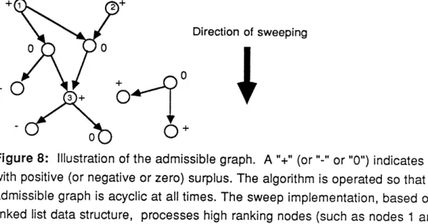
Figure 8 depicts the sweep implementation.
Proposition 3. Under the sweep implementation, if the initial admissable graph is acyclic and the initial node order is compatible with it, then the total complexity of the sweep implementation is O(N2(0/e + N)).
Proof: Combining the results of lemmas 6, 7, and 11, we find that the dominant term is
O(N2([3/e + N)), corresponding to the nonsaturating pushes (since we assume at most one arc in each direction between any pair of nodes, A = O(N2)). The only other work performed by the algorithm is in maintaining the linked list, which involves only 0(1) work per price rise, and scanning down this list in the course of each cycle, which involve O(N) work per cycle. As there are O(N2(1/e + N)) price rises and O(N(f/e + N)) cycles, both these leftover terms work out to O(N2(3P/e + N)). QED.
A straightforward way of meeting the conditions of proposition 3 is to choose p arbitrarily and set fij = cij for all active (as opposed to e-active) arcs and fij = bij for all inactive ones. Then there will be no admissible arcs, and the initial admissible graph will be trivially acyclic. The initial node order may then be chosen arbitrarily.
The above proof also gives insight into the complexity of the method when other orders are used. At worst, only one node will be added to NOin each cycle, and hence that there may be
Q(N) cycles between successive price rises. In the absence of further analysis, one concludes that the complexity of the algorithm is a factor of N worse.
An alternate approach is to eschew cycles, and simply maintain a data structure representing the set of all nodes with positive surplus. [30] shows that a broad class of implementations of this kind have complexity O(NA(3/£ + N)). (Actually, these results are embedded in a scaling analysis, but the outcome is equivalent.)
We now give an upper bound on the complexity of the pure (unscaled) e-relaxation algorithm, using the sweep implementation. Suppose we set the initial price vector pO to zero and choose f so that there are initially no admissible arcs. Then a crude upper bound on
1
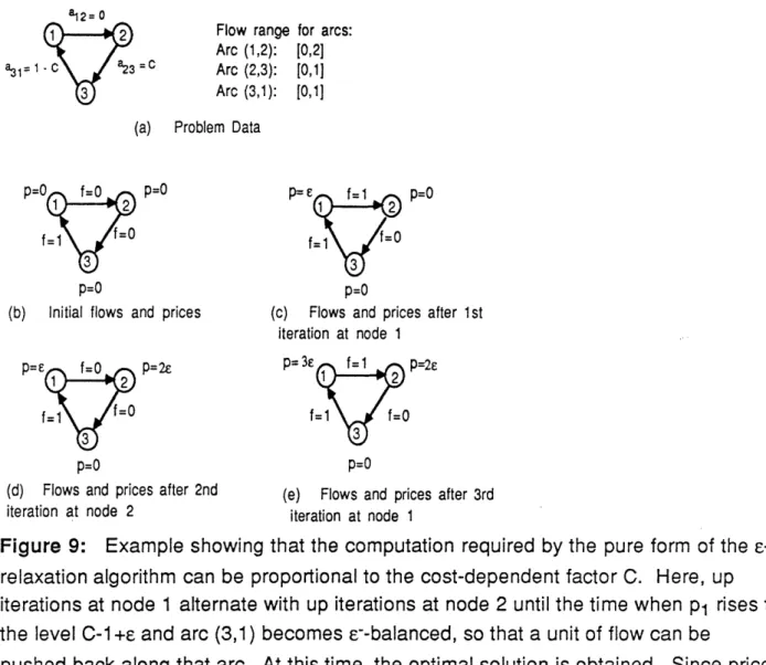
is NC, where C is the maximum absolute value of the arcs costs, as in section 2. Letting e = 1/(N + 1) to assure optimality upon termination, we get an overall complexity bound of O(N4C). Figure 9demonstrates that the time taken by the method can indeed vary linearly with C, so the algorithm is exponential.
Note also that any upper bound P* on [3 provides a means of detecting infeasibility: If the problem instance (MCF) is not feasible, then the algorithm may abort in step 4 of some up iteration, or some group of prices may diverge to +oo. If any price increases by more than
3*
+ N£, then we may conclude such a divergence is happening, and halt with a conclusion of infeasibility. Thus, the total complexity may be limited to O(N2(f*/e + N)), even without the assumption of feasibility. NC is always a permissible value for3*.
5.
Application to Maximum Flow
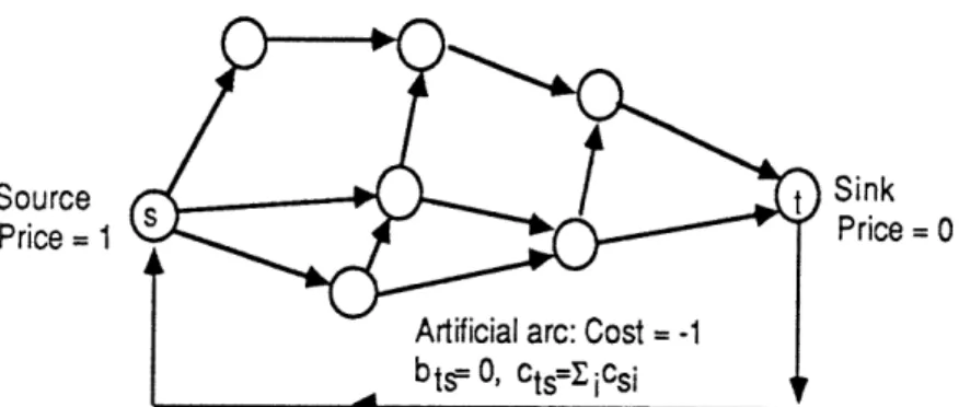
For classes of problems with special structure, a better estimate of 1(pQ) may be possible. As an example, consider the max-flow problem formulation shown in Figure 10. The artificial arc (t, s) connecting the sink t with the source s has cost coefficient -1, and flow bounds bts = 0 and cts = Lie N Csi . We assume that aij = 0 and bij = O < cij for all other arcs (i, j), and that si= 0 for all i. We apply the e-relaxation algorithm with initial prices and arc flows satisfying e-complementary slackness, where £ = l/(N+1). The initial prices may be arbitrary, so long as there is on 0(1) bound on how much they differ. Then we obtain dH(p0) = 0(1) for all paths H, 1(p0) = 0(1), and an O(N3) complexity bound. Note we may choose any positive value for £ and negative values for ats, as long as £ = -ats/(N+l) (more generally £ = -ats/(l+ Largest number of arcs in a cycle containing (t,s))).
Applied like this to the maximum flow problem, e-relaxation yields an algorithm resembling the maximum flow algorithm of [26]-[27], and having the same complexity. However, it has only one
phase. The first phase of the procedure of [26]-[27] may in hindsight considered to be an
application of e-relaxation with £ = 1 to the (infeasible) formulation of the maximum flow problem in which one considers all arcs costs to be zero, ss = -o, and st = + oo.
6.
Scaling Procedures
In general, some sort of scaling procedure ([ 18], [23], [38]) must be used to make the c-relaxation algorithm polynomial. The basic idea is to divide the solution of the problem into a polynomial number of subproblems (also called scales or phases) in which £-relaxation is applied,
with 3(pO)/c being polynomial within each phase. The original analysis of this type, as we have mentioned, is due to Goldberg ([28] and, with Tarjan, [30]), who used e-scaling. In order to be sure that all price rises are by gQ(£) amounts, both these papers use the broadbanding variant of e-relaxation as their principal subroutine (though they also present alternatives which are not dual coordinate ascent methods). Here, we will present an alternative cost scaling procedure that results in an overall complexity of O(N3log NC).
6.1. Cost Scaling
Consider the problem (SMCF) obtained from (MCF) by multiplying all arc costs by N+1, that is, the problem with arc cost coefficients
aij' = (N+1)aij for all (i, j). (31)
If the pair (f ', p') satisfies 1-complementary slackness (namely e-complementary slackness with £2= 1) with respect to (SMCF), then clearly the pair
(f, p)=(f', p'/(N+l)) (32)
satisfies (N+1)-l-complementary slackness with respect to (MCF), and hence f' is optimal for (MCF) by Proposition 1. In the scaled algorithm, we seek a solution to (SMCF) obeying 1-complementary slackness.
Let
M = Llog2 (N+1)CJ + 1 = O(log(NC)) . (33)
In the scaled algorithm, we solve M subproblems, in each case using the sweep implementation of c-relaxation. The mth subproblem is a minimum cost flow problem where the cost coefficient of
each arc (i, j) is
aij(m) = Trunc( aij'/ (2M - m) ), (34)
where Trunc( · ) denotes integer rounding in the direction of zero, that is, down for positive and up for negative numbers. Note that aij(m) is the integer consisting of the m most significant bits in the
M-bit binary representation of aij'. In particular, each aij(l) is 0, +1, or -1, while aij(m+l) is obtained by doubling aij(m) and adding (subtracting) one if the (m+l)st bit of the M-bit representation of aij' is a one and aij' is positive (negative). Note also that
aij(M) = aij', (35)
so the last problem of the sequence is (SMCF).
For each subproblem, we apply the unscaled version of the algorithm with e = 1, yielding upon termination a pair (ft(m), pt(m)) satisfying 1-complementary slackness with respect to the cost coefficients aij(m).
The starting price vector for the (m+1)st problem (m = 1, 2, .... , M-1) is
pO(m+1) = 2pt(m). (36)
Doubling pt(m) as above roughly maintains complementary slackness since aij(m) is roughly doubled when passing to the (m+l)st problem. Indeed it can be seen that every arc that was 1 balanced (1 active, 1 inactive) upon termination of the algorithm for the mth problem will be 3 -balanced (1 - active, 1 - inactive, respectively) at the start of the (m+1)st problem.
The starting flow vector fO(m+l) for the (m+l)st problem may be obtained from ft(m) in any way that obeys 1-complementary slackness, keeps the admissible graph acyclic, and allows straightforward construction of a compatible node order. The simplest way to do this is to set
f0ij(m+l) = ftij(m) for all balanced arcs (i, j), (37a) foij(m+l) = cij for all active arcs (i, j), and (37b)
f0ij(m+l) = bij for all inactive arcs (i, j). (37c)
This procedure implies that the initial admissible graph for the (m+l)st problem has no edges, and so an arbitrary node order (such as the one from the end of the last subproblem) may be used. A procedure that does not alter as many arc flows (and hence likely to generate fewer nodes with
nonzero surplus) is to set
f0ij(m+l) = cij for all 1 - active arcs (i, j), f0ij(m+l) = bij for all 1 - inactive arcs (i, j),
f0ij(m+l) = cij for all 1+ - active arcs (i, j) that were not admissible at the end of the previous phase,
f0ij(m+l) = bij for all 1- - active arcs (i, j) that were not admissible at the end of the previous phase, and
f0ij(m+l) = ftij(m) for all other arcs (i, j).
In this case, the edge set of the new admissible graph will be a subset of that prevailing at the end of subproblem m, hence the new graph will be acyclic. Furthermore, the node order at the end of phase m will be compatible with the new admissible graph, and may be used as the starting node order for phase m+l. For the first subproblem, however, there is no prior admissible graph, so the procedure (37a-c) must be used, and the initial node order can be arbitrary. The starting prices may be arbitrary so long as there is an O(N) bound on how much they can differ.
6.2. Analysis
Using the analysis of section 4, it is now fairly straightforward to find the complexity of the scaled form of the algorithm as outlined above.
Proposition 4. The complexity of the scaled form of the c-relaxation algorithm is O(N3log NC).
Proof: Using Proposition 3 and e = 1, the complexity of the scaled form of the algorithm is O(N2B + N3M) where
M
B =
X,
m(p0(m)) (38)m= 1
and [3m(-) is defined by (22) - (24) but with the modified cost coefficients aij(m) replacing aij in (22). We show that
3m(p0(m)) = O(N) for all m, (39)
thereby obtaining an O(N3 log NC) complexity bound, as M = O(log NC). At the beginning of the first subproblem, we have
pi-Pj=O(l), aij(l) = O(l) for all arcs (i, j), (40) so we obtain dH(p 0(l)) = O(N) for all H, and l3 (pO(1)) = O(N). The final flow vector ft(m) obtained from the m-th problem is feasible, and together with pO(m+l) it may be easily seen to satisfy 3-complementary slackness. It follows from Lemma 4(a) that
13m+l(p 0(m+l)) < 3(N-1) = O(N) . (41)
It then follows that B = O(NM), and the overall complexity is O(N3 log NC). QED.
Of course, many variations are possible. For example, it is not necessary to use the sweep implementation to achieve polynomial complexity. Also, it is possible to increase the accuracy of the cost data by factors other than two. Our limited computational experiments on the NETGEN
family of problems seems to indicate that it is more efficient to increase accuracy by a factor between 4 and 8 between consecutive subproblems.
6.3. Further Developments in Scaling
Other recent developments in scaling include Gabow and Tarjan's [25], which is also a cost scaling method. Ahuja and Orlin, working jointly with Goldberg and Tarjan, have also developed a double scaling method which scales not only £, but also surpluses and arc capacities, and has complexity O(NA (log log U) log NC), where U is the maximum arc capacity cij [3] .
Furthermore, analysis in [30], drawing on some ideas of Tardos [42], shows that a strongly polynomial bound (that is, one polynomial in N and A) may be placed on a properly implemented
scaling algorithm.
7.
The Auction Algorithm
7.1. Motivation
Despite the good theoretical complexity bounds available for the scaled form of e-relaxation and its relatives, dual coordinate algorithms have not yet proven themselves to be good performers in practice. Although nonsaturating pushes are the theoretical bottleneck in the algorithm, they present little problem in practice. We have observed that typically there are only a few flow alterations between successive price rises. The real problem with the algorithm is the tendency of prices to rise at the theoretically minimum rate - by only £ or 2e per price change. This is the phenomenon of price haggling. Essentially, the algorithm is following a "staircase" path in the dual (such as in figure 5), where the individual steps are very small.
Without scaling, the amount of price haggling can be exponential (as in figure 9), so scaling is clearly necessary to make e-relaxation efficient. However, even with scaling, our computational experiments have shown that haggling is still a serious difficulty. It often manifests itself in a prolonged "endgame" at the close of each subproblem, in which only a handful of nodes have positive surplus at any given time. Our experiments have also shown that degenerate price rises cause a dramatic decrease in price haggling, often by orders of magnitude; we contend that they will be necessary in any practical implementation of algorithms of this type.
Even with scaling and degenerate steps, however, we have found e-relaxation to be several orders of magnitude slower than state-of-the-art sequential codes such as RELAX for large problems. We have not yet experimented with broadbanding and c-scaling as opposed to cost scaling; although these techniques may offer some speed-up, we suspect it will not be dramatic. Also, the potential speed-up obtainable by a parallel implementation, as roughly indicated by the
![Figure 6: Illustration of an up iteration involving a single node s with four incident arcs (1 ,s), (3,s), (s,2), and (s,4), with feasible arc flow ranges [1,20], [0,20], [0,10], and](https://thumb-eu.123doks.com/thumbv2/123doknet/14753633.581373/47.933.105.733.132.883/figure-illustration-iteration-involving-single-incident-feasible-ranges.webp)