HAL Id: hal-02084080
https://hal.archives-ouvertes.fr/hal-02084080
Submitted on 7 Jan 2021
HAL is a multi-disciplinary open access
archive for the deposit and dissemination of
sci-entific research documents, whether they are
pub-lished or not. The documents may come from
teaching and research institutions in France or
abroad, or from public or private research centers.
L’archive ouverte pluridisciplinaire HAL, est
destinée au dépôt et à la diffusion de documents
scientifiques de niveau recherche, publiés ou non,
émanant des établissements d’enseignement et de
recherche français ou étrangers, des laboratoires
publics ou privés.
Testing of Dynamical Models Against the Real Kuiper
Belt
Samantha Lawler, J. Kavelaars, Mike Alexandersen, Michele Bannister, Brett
Gladman, Jean-Marc Petit, Cory Shankman
To cite this version:
Samantha Lawler, J. Kavelaars, Mike Alexandersen, Michele Bannister, Brett Gladman, et al..
OS-SOS: X. How to Use a Survey Simulator: Statistical Testing of Dynamical Models Against the Real
Kuiper Belt. Frontiers in Astronomy and Space Sciences, Frontiers Media, 2018, 5,
�10.3389/fs-pas.2018.00014�. �hal-02084080�
Edited by: Lorenzo Iorio, Ministry of Education, Universities and Research, Italy Reviewed by: J. Allyn Smith, Austin Peay State University, United States Akos Bazso, Universität Wien, Austria *Correspondence: Samantha M. Lawler [email protected]
†Present Address:
Cory Shankman, City of Toronto, Toronto, ON, Canada
Specialty section: This article was submitted to Fundamental Astronomy, a section of the journal Frontiers in Astronomy and Space Sciences Received: 31 January 2018 Accepted: 30 April 2018 Published: 16 May 2018 Citation: Lawler SM, Kavelaars JJ, Alexandersen M, Bannister MT, Gladman B, Petit J-M and Shankman C (2018) OSSOS: X. How to Use a Survey Simulator: Statistical Testing of Dynamical Models Against the Real Kuiper Belt. Front. Astron. Space Sci. 5:14. doi: 10.3389/fspas.2018.00014
OSSOS: X. How to Use a Survey
Simulator: Statistical Testing of
Dynamical Models Against the Real
Kuiper Belt
Samantha M. Lawler1*, J. J. Kavelaars1,2, Mike Alexandersen3, Michele T. Bannister4,
Brett Gladman5, Jean-Marc Petit6and Cory Shankman1,2†
1NRC-Herzberg Astronomy and Astrophysics, National Research Council of Canada, Victoria, BC, Canada,2Department of
Physics and Astronomy, University of Victoria, Victoria, BC, Canada,3Institute of Astronomy and Astrophysics, Academia
Sinica, Taipei, Taiwan,4Astrophysics Research Centre, Queen’s University Belfast, Belfast, United Kingdom,5Department of
Physics and Astronomy, The University of British Columbia, Vancouver, BC, Canada,6Institut UTINAM, UMR 6213 Centre
National de la Recherche Scientifique-Université de Franche Comté, Besançon, France
All surveys include observational biases, which makes it impossible to directly compare properties of discovered trans-Neptunian Objects (TNOs) with dynamical models. However, by carefully keeping track of survey pointings on the sky, detection limits, tracking fractions, and rate cuts, the biases from a survey can be modeled in Survey Simulator software. A Survey Simulator takes an intrinsic orbital model (from, for example, the output of a dynamical Kuiper belt emplacement simulation) and applies the survey biases, so that the biased simulated objects can be directly compared with real discoveries. This methodology has been used with great success in the Outer Solar System Origins Survey (OSSOS) and its predecessor surveys. In this chapter, we give four examples of ways to use the OSSOS Survey Simulator to gain knowledge about the true structure of the Kuiper Belt. We demonstrate how to statistically compare different dynamical model outputs with real TNO discoveries, how to quantify detection biases within a TNO population, how to measure intrinsic population sizes, and how to use upper limits from non-detections. We hope this will provide a framework for dynamical modelers to statistically test the validity of their models.
Keywords: Kuiper belt, trans-Neptunian objects, observational surveys, survey biases, dynamical models, numerical methods, statistics
1. INTRODUCTION
The orbital structure, size frequency distribution, and total mass of the trans-Neptunian region of the Solar System is an enigmatic puzzle.Fernandez (1980)described an expected distribution for this region based on the mechanisms for the delivery of cometary material into the inner Solar System. Even before the first Kuiper belt object after Pluto was discovered, (1992 QB1;Jewitt and
Luu, 1993, 1995), it was theorized that dynamical effects produced by the mass contained in this region could in principle be detectable (Hamid et al., 1968). The first discoveries made it clear that extracting precise measurements of the orbital and mass distributions from this zone of the Solar System would require careful analysis.
Major puzzles in the Solar System’s history can be explored if one has accurate knowledge of the distribution of material in this zone. Examples include: the orbital evolution of Neptune (e.g.,
Malhotra, 1993), the large scale re-ordering of the Solar System (e.g., Thommes et al., 1999; Gomes et al., 2005), the process of planetesimal accretion (e.g.,Stern, 1996; Davis and Farinella, 1997), the production of cometary size objects via collisional processes (e.g. Stern, 1995) and their delivery into the inner Solar System (Duncan et al., 1988), and the stellar environment in which the Sun formed (e.g., Brunini and Fernandez, 1996; Kobayashi and Ida, 2001). Our goal as observers is to test these models and their consequences by comparison to the Solar System as we see it today. Given the sparse nature of the datasets and the challenges of detecting and tracking trans-Neptunian objects (TNOs), a strong statistical framework is required if we are to distinguish between these various models.
The presence of large-scale biases in the detected sample of TNOs has been apparent since the initial discoveries in the Kuiper belt, and multiple approaches have been used to account for these biases. Jewitt and Luu (1995) use Monte-Carlo comparisons of Kuiper belt models to their detected sample to estimate the total size of the Kuiper belt, taking into account the flux limits of their survey. Similarly Irwin et al. (1995) estimate the flux limits of their searches and use these to weight their detections and, combining those with the results reported in Jewitt and Luu (1995), provide an estimate of the luminosity function of the region.Gladman et al. (1998)provide a Bayesian-based analysis of their detected sample, combined with previously published surveys, to further refine the measurement of the luminosity function of the Kuiper belt.Trujillo et al. (2001)
determined the size, inclination, and radial distributions of the Kuiper belt by weighting the distribution of observed TNOs based on their detectability and the fraction of the orbits that were contained within the survey fields.Bernstein et al. (2004)
refined the maximum-likelihood approach when they extended the measurement of the size distribution to smaller scales and determined statistically significant evidence of a break in the shape of the Kuiper belt luminosity function, later developed further by the deeper survey ofFraser and Kavelaars (2009). A similar approach is taken inAdams (2010)who make estimates of the underlying sampling by inverting the observed distributions. Other recent results for Kuiper belt subpopulations include
Schwamb et al. (2009), who use Monte Carlo sampling to estimate detectability of Sedna-like orbits, and Parker (2015), who uses an approximate Bayesian computation approach to account for unknown observation biases in the Neptune Trojans. Each of these methods relies on backing out the underlying distributions from a detected sample.
Carefully measuring the true, unbiased structure of the Kuiper belt provides constraints on exactly how Neptune migrated through the Kuiper belt. Two main models of Neptune’s migration have been proposed and modeled extensively. Pluto’s eccentric, resonant orbit was first explained by a smooth migration model for Neptune (Malhotra, 1993, 1995). Larger scale simulations (Hahn and Malhotra, 2005) showed this to be a viable way to capture many TNOs into Neptune’s mean-motion resonances. The so-called “Nice model” was proposed
as an alternate way to destroy the proto-Kuiper belt and capture many TNOs into resonances (Levison et al., 2008). In this model, the giant planets undergo a dynamical instability that causes Neptune to be chaotically scattered onto an eccentric orbit that damps to its current near-circular orbit while scattering TNOs and capturing some into its wide resonances (Tsiganis et al., 2005). Due to the chaotic nature of this model, reproducing simulations is difficult and many variations on the Nice model exist (e.g., Batygin et al., 2012; Nesvorný et al., 2013). One very recent and promising variation on the Nice model scenario includes the gravitational effects of fairly large (∼Pluto-sized) bodies that cause Neptune’s migration to be “grainy,” having small discrete jumps as these larger bodies are scattered (Nesvorný and Vokrouhlický, 2016). More dramatically, even larger planetary-scale objects could have transited and thus perturbed the young Kuiper belt (Petit et al., 1999; Gladman and Chan, 2006; Lykawka and Mukai, 2008; Silsbee and Tremaine, 2018)
The level of detail that must be included in Neptune migration scenarios is increasing with the number of discovered TNOs with well-measured orbits; some recent examples of literature comparisons between detailed dynamical models and TNO orbital distributions are summarized here. Batygin et al. (2011),Dawson and Murray-Clay (2012), andMorbidelli et al. (2014) all use slightly different observational constraints to place limits on the exact eccentricity and migration distance of Neptune’s orbit in order to preserve the orbits of cold classical TNOs as observed today.Lawler and Gladman (2013)
test the observed distribution of Kozai Plutinos against the output from a smooth Neptune migration model (Hahn and Malhotra, 2005) and a Nice model simulation (Levison et al., 2008), finding that neither model produces sufficiently high inclinations. Nesvorný (2015a) shows that the timescale of Neptune’s migration phase must be fairly slow (&10 Myr) in order to replicate the observed TNO inclination distribution, and
Nesvorný (2015b)shows that including a “jump” in Neptune’s semimajor axis evolution can create the “kernel” observed in the cold classical TNOs (first discussed in Petit et al., 2011). Pike et al. (2017)compare the output of a Nice model simulation (Brasser and Morbidelli, 2013) with scattering and resonant TNOs, finding that the population ratios are consistent with observations except for the 5:1 resonance, which has far more known TNOs than models would suggest (Pike et al., 2015). Using the observed wide binary TNOs as a constraint on dynamical evolution suggests that this fragile population formed in-situ (Parker and Kavelaars, 2010) or was emplaced gently into the cold classical region (Fraser et al., 2017). Regardless of the model involved, using a Survey Simulator is the most accurate and statistically powerful way to make use of model TNO distributions from dynamical simulations such as these to gain constraints on the dynamical history of the Solar System.
In this chapter, we discuss what it means for a survey to be “well-characterized” (section 2) and explain the structure and function of a Survey Simulator (section 2.1). In section 3, we then give four explicit examples of how to use a Survey Simulator, with actual dynamical model output and real TNO data. We hope this chapter provides an outline for others to follow.
2. WELL-CHARACTERIZED SURVEYS
A well-characterized survey is one in which the survey field pointings, depths, and tracking fractions at different magnitudes and on-sky rates of motion have been carefully measured. The largest well-characterized TNO survey to date is the Outer Solar System Origins Survey (OSSOS; Bannister et al., 2016), which was a large program on the Canada-France-Hawaii Telescope (CFHT) carried out over five years, and was specifically planned with the Survey Simulator framework in mind. OSSOS builds on the methodology of three previous well-characterized surveys: the Canada-France Ecliptic Plane Survey (CFEPS; Jones et al., 2006; Kavelaars et al., 2008b; Petit et al., 2011), the CFEPS high-latitude component (Petit et al., 2017), and the survey of Alexandersen et al. (2016). The survey design is discussed extensively in those papers; the OSSOS survey outcomes and parameters in particular are presented in detail in Bannister et al. (2016, 2018). We here summarize the main points that are important for creating a well-characterized survey.
These well-characterized surveys are all arranged into observing “blocks”: many individual camera fields tiled together into a continuous block on the sky (the observing blocks for OSSOS are each ∼10–20 square degrees in size). The full observing block is covered during each dark run (when the Moon is closest to new) for the 2 months before, 2 months after, and during the dark run closest to opposition for the observing block. The observing cadence is important for discovering and tracking TNOs, which change position against the background stars on short timescales. The time separation between imaging successive camera fields inside each observing block must be long enough that significant motion against background stars has occurred for TNOs, but not so long that the TNOs have moved too far to be easily recovered by eye or by software. OSSOS used triplets of images for each camera field, taken over the course of 2 h. The exposure times are chosen as a careful compromise between photometric depth and limiting trailing1 of these moving sources. The images are searched for moving objects by an automated and robustly tested moving object pipeline (CFEPS and OSSOS used the software pipeline described inPetit et al., 2004), and all TNO candidates discovered by the software are visually inspected. Prior to searching the images, artificial sources (whose flux and image properties closely mimic the real sample) are inserted into the images. The detection of these implanted sources marks the fundamental calibration and characterization of the survey block in photometric depth, detection efficiency, and tracking efficiency. Each observing block has a measured “filling factor” that accounts for the gaps between CCD chips. Detection and tracking efficiencies are measured at different on-sky rates of motion using implanted sources in the survey images, analyzed along with the real TNO data. This process is repeated for each observing block, so each block has known magnitude limits, filling factors, on-sky coverage, and detection and tracking efficiencies at different on-sky rates of
1We note that clever algorithms can be used to obtain accurate photometry from trailed sources (e.g.,Fraser et al., 2016).
motion. These are then parameterized and become part of the Survey Simulator.
The tracking of the discovered sample provides another opportunity for biases to enter and the process must be closely monitored. A survey done in blocks of fields that are repeated ∼monthly removes the need to make orbit predictions based on only a few hours of arc from a single night’s discovery observations. Such short-arc orbit predictions are notoriously imprecise, and dependence on them ensures that assumptions made regarding orbit distribution will find their way into the detected sample as biases. For example, a common assumption for short-arc orbits is a circular orbit. If follow-up observations based on this circular orbital prediction are attempted with only a small area of sky coverage, then those orbits whose Keplerian elements match the input assumptions will be preferentially recovered, while those that do not will be preferentially lost, resulting in a discovery bias against non-circular orbits. Correcting for this type of ephemeris bias is impossible. Several of the large-sample TNO surveys had short arcs on a high fraction of the detections; this introduces unknown tracking biases into the sample that cannot be reproduced in a Survey Simulator because the systematic reasons for object loss (ephemeris bias,
Jones et al., 2010) cannot be modeled as random. Repeatedly observing the same block of fields, perhaps with some adjustment for the bulk motion of orbits, helps ensure that ephemeris bias is kept to a minimum. In the OSSOS project we demonstrate the effectiveness of this approach by managing to track essentially all TNOs brighter than the flux limits of the discovery sequences (only 2 out of 840 TNOs were not tracked2;Bannister et al., 2018).
Schwamb et al. (2010)is an example of a large-scale TNO survey from outside our collaboration that is well-characterized. It has a high tracking fraction and a published pointing history. However, it has a comparatively noisy and low-resolution detection efficiency function, thus we do not include it in our Survey Simulator analysis here. Other large sample size TNO surveys have either unpublished pointings or indications of low tracking fractions leading to unrecoverable ephemeris bias.
A well-characterized survey will have flux limits in each observing block from measurements of implanted artificial objects, equal sensitivity to a wide range of orbits, and a known spatial coverage on the sky. A Survey Simulator can now be configured to precisely mimic the observing process for this survey.
2.1. The Basics of a Survey Simulator
A Survey Simulator allows models of intrinsic Kuiper Belt distributions to be forward-biased to replicate the biases inherent in a given well-characterized survey. These forward-biased simulated distributions can then be directly compared with real TNO detections, and a statement can be made about whether or not a given model is statistically consistent with the known TNOs. One particular strength of this approach is that the effect of non-detection of certain orbits can be included in the analysis.
2The two objects that were not tracked are d <15 AU Centaurs whose high on-sky rates of motion caused them to shear off the fields. The possibility of such shearing loss is accounted for in the Survey Simulator.
Methods that rely on the inversion of orbital distributions are, by their design, not sensitive to a particular survey’s blind spots.
Directly comparing a model with a list of detected TNOs (for example, from the Minor Planet Center database), with a multitude of unknown detection biases, can lead to inaccurate and possibly false conclusions. Using a Survey Simulator avoids this problem completely, with the only downside being that comparisons can only be made using TNOs from well-characterized surveys. Fortunately, the single OSSOS survey contains over 800 TNOs, and the ensemble of well-characterized affiliated surveys contains over 1100 TNOs with extremely precisely measured orbits (Bannister et al., 2018). This is roughly one third of the total number of known TNOs, and one half of the TNOs with orbits that are well-determined enough to perform dynamical classification.
At its most basic, a Survey Simulator must produce a list of instantaneous on-sky positions, rates of motion, and apparent magnitudes. These are computed by assigning absolute magnitudes to simulated objects with a given distribution of orbits. These apparent magnitudes, positions, and rates of motion are then evaluated to determine the likelihood of detection by the survey, and a simulated detected distribution of objects is produced. The OSSOS Survey Simulator follows this basic model, but takes into account more realities of survey limitations. It is the result of refinement of this Survey Simulator software through several different well-characterized surveys: initially the CFEPS pre-survey (Jones et al., 2006), then CFEPS (Kavelaars et al., 2008a; Petit et al., 2011), thenAlexandersen et al. (2016), and finally OSSOS (Bannister et al., 2016). The OSSOS Survey Simulator software and methodology are now robustly tested, and are presented below.
2.2. The Details of the OSSOS Survey
Simulator
While the methodology presented here is specific to the OSSOS Survey Simulator, by measuring on sky pointings, magnitude limits, and tracking fractions, a Survey Simulator can be built for any survey. The Survey Simulator for the OSSOS ensemble of well-characterized surveys is available as a package3, and the
list of observed characteristics of the TNOs discovered in these surveys is published inBannister et al. (2018). To forward-bias a distribution of objects to allow statistical comparison with the real TNO discoveries in the surveys, the OSSOS Survey Simulator uses the following steps. The instantaneous on-sky position, rate of motion, and apparent magnitude are computed from an orbit, position, and H-magnitude, and can be written to a file that contains the “drawn” simulated objects. This “drawn” file then represents the instantaneous intrinsic distribution of simulated objects. The Survey Simulator evaluates whether each simulated object falls within one of the observing blocks of the survey, and if so, uses the tracking and detection efficiency files for that observing block to calculate whether this object would be detected. If it is detected, the properties of this object are written to a file containing the simulated detections. A very small fraction of on-sky motion rates were detected and not tracked in the real
3https://github.com/OSSOS/SurveySimulator
survey (Centaurs sometimes shear off the field due to their high rate of motion), which is accounted for in the Survey Simulator. The simulated objects are written to the simulated tracked object file with probabilities reflecting this.
The user must supply the Survey Simulator with a routine that generates an object with orbital elements and an absolute H magnitude. How these are generated is free for the user to decide. The user may edit the source software to include generation of orbits and absolute magnitudes within the Survey Simulator, but it is recommended that a separate script is used in conjunction with the unedited Survey Simulator. The software package comes with a few examples, and details are provided in the following paragraph showing how we on the OSSOS team have implemented the generation of simulated TNOs.
The orbital elements of an object can be determined in a variety of ways. The Survey Simulator can choose an orbit and a random position within that orbit, either from a list of orbits (as would be produced by a dynamical model) or from a parametric distribution set by the user. Orbits from a list can also be easily “smeared,” that is, variation is allowed within a fraction of the model orbital elements, in order to smooth a distribution or produce additional similar orbits (however, one must be careful that the distribution is dominated by the original list of orbits, and not by the specifics of the smearing procedure). To determine the likely observed magnitude of the source, an absolute H magnitude is assigned to this simulated object, chosen so as to replicate an H-distribution set by the user. Tools and examples are provided to set the H-distribution as a single exponential distribution, to include a knee to a different slope at a given H magnitude (see, for example,Fraser et al., 2014), or to include a divot in the H-distribution (as inShankman et al., 2016; Lawler et al., 2018) The H-distribution parameter file also sets the maximum and minimum H values that will be simulated. The smallest H-magnitude (i.e., largest diameter) is not as important because it is set by the distribution itself. But the largest H-magnitude (i.e., smallest diameter) is important to match to the population being simulated. If the maximum H-magnitude is smaller than that of the largest magnitude TNO in the observational sample one wants to simulate, then the distribution won’t be sensitive to this large H-magnitude tail. If the maximum H value is much larger than that of the largest magnitude TNO in the sample, it is simply a waste of computational resources, since the simulation will include many objects that were too faint to be detected in the survey. This does, however, expose a strength of the Survey Simulator, as we can learn from these faint detections that a hidden reservoir of small objects might exist.
The process of drawing simulated objects and determining if they would have been detected by the given surveys is repeated until the desired number of simulated tracked or detected objects is produced by the Survey Simulator. The desired number of simulated detected objects may be the same as the number of real detected TNOs in a survey in order to measure an intrinsic population size (as demonstrated in section 3.3), or an upper limit on a non-detection of a particular subpopulation (section 3.4), or it may be a large number in order to test the rejectability of an underlying theoretical distribution (as
demonstrated in sections 3.1) or to quantify survey biases in a given subpopulation (section 3.2).
3. EXAMPLES OF SURVEY SIMULATOR
APPLICATIONS
Here we present four examples of different ways to use the Survey Simulator to gain statistically valuable information about TNO populations. In section 3.1, we demonstrate how to use the Survey Simulator to forward-bias the output of dynamical simulations and then statistically compare the biased simulation with a distribution of real TNOs. In section 3.2, we use the Survey Simulator to build a parametric intrinsic distribution and then bias this distribution by our surveys, examining survey biases for a particular TNO subpopulation in detail. The Survey Simulator can also be used to measure the size of the intrinsic population required to produce a given number of detections in a survey; this is demonstrated in section 3.3. And finally, in section 3.4, we demonstrate a handy aspect of the Survey Simulator: using non-detections from a survey to set statistical upper limits on TNO subpopulations. We hope that these examples will prove useful for dynamical modelers who want a statistically powerful way to test their models.
3.1. Testing the Output of a Dynamical
Model: The Outer Solar System With a
Distant Giant Planet or Rogue Planet
This example expands on the analysis of Lawler et al. (2017), which presents the results of three different dynamical emplacement simulations of the distant Kuiper Belt. Here we analyze these three dynamical simulations and also an additional emplacement model that includes a “rogue planet” that is ejected early in the Solar System’s history (Gladman and Chan, 2006). The outputs from these four dynamical TNO emplacement simulations are run through the OSSOS Survey Simulator and compared with the high pericenter TNOs discovered by OSSOS. The four emplacement simulation scenarios analyzed here include the following conditions:
1. The four giant planets and including the effects of Galactic tides and stellar flybys (simulation fromKaib et al., 2011) 2. The four giant planets with an additional 10 Earth mass planet
having a = 250 AU and e = 0 (based on a theory proposed inTrujillo and Sheppard, 2014), also including the effects of Galactic tides and stellar flybys (simulation fromLawler et al., 2017).
3. The four giant planets with an additional 10 Earth mass planet having a = 500 AU and e = 0.5 (based on a theory proposed in Batygin and Brown, 2016), also including the effects of Galactic tides and stellar flybys (simulation fromLawler et al., 2017).
4. The four giant planets and an additional 2 Earth mass rogue planet that started with a = 35 AU and q = 30 AU, which was ejected after ∼200 Myr (simulation fromGladman and Chan, 2006).
The papers which have recently proposed the presence of a distant undiscovered massive planet (popularly referred to as “Planet 9”; Trujillo and Sheppard, 2014; Batygin and Brown, 2016) rely on published detections of large semimajor axis (a), high pericenter distance (q) TNOs, which have extreme biases against detection in flux-limited surveys4. These large-a, high-q
TNOs are drawn from different surveys, with unpublished and thus unknown observing biases. The Minor Planet Center (MPC) Database, which provides a repository for TNO detections, does not include information on the pointings or biases of the surveys that detected these TNOs. Sample selection caused by survey depth and sky coverage can be non-intuitive, caused by weather, galactic plane avoidance, and telescope allocation pressure, among other possibilities (Sheppard and Trujillo, 2016; Shankman et al., 2017). Thus the assumption can not be made that a collection of TNOs from different surveys will be bias-free. Further, the detected sample of objects in the MPC Database provides no insight into the parts of the sky where a survey may have looked and found nothing, nor to strong variation in flux sensitivity that occurs due to small variations in image quality.
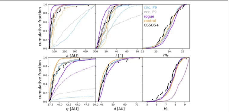
Here we demonstrate how to use the results of well-characterized surveys to compare real TNO detections to the output of a dynamical model, comprising a list of orbits. We visualize this output with a set of cumulative distributions. Figure 1 shows cumulative distributions in six different observational parameters: semimajor axis a, inclination i, apparent magnitude in r-band mr, pericenter distance q,
distance at detection d, and absolute magnitude in r-band Hr.
The outputs from the four emplacement models are shown by different colors in the plot, with the intrinsic distributions shown as dotted lines, and the forward-biased simulated detection distributions as solid lines. These intrinsic distributions have all been cut to only include the pericenter and semimajor axis range predicted byBatygin and Brown (2016)to be most strongly affected by a distant giant planet: q > 37 AU and 50 < a < 500 AU.
We cannot directly compare the output from these dynamical simulations covering such a huge range of a and q to real TNOs because the observing biases present in the detected TNO distributions are severe. Using a survey simulator combined with a carefully characterized survey, however, allows us to impose the observing biases onto the simulated sample and determine what the detected simulated sample would have been. We use the OSSOS Survey Simulator and the q > 37 AU, 50 < a < 500 AU TNOs discovered by the OSSOS ensemble in this example (Figure 1).
The solid lines in Figure 1 show the forward-biased simulated detections from the Survey Simulator, and the black points show the real TNOs detected in the OSSOS ensemble with the same a and q cut. These can now be directly compared, as the same biases have been applied. The effect of observing biases varies widely among the six parameters plotted, and can be
4Brown (2017)does attempt a numerical simulation to calculate likelihood of detection for different orbital parameters in the high-q population, but this is backing out the underlying distribution in the underlying sample and still relies on assumptions about the unknown sensitivity and completeness of the surveys.
FIGURE 1 | Cumulative distributions of TNOs in six different parameters: semimajor axis a, inclination i, apparent r-band magnitude mr, pericenter distance q, distance at detection d, and absolute magnitude in r-band Hr. The result of four different emplacement models are presented: the known Solar System (orange), the Solar System plus a circular orbit Planet 9 (blue), or plus an eccentric orbit Planet 9 (gray), and a “rogue” planet simulation (purple). The intrinsic model distributions are shown with dotted lines, and the resulting simulated detections in solid lines. Black circles show non-resonant TNOs discovered by the OSSOS ensemble having q >37 AU and 50 < a < 500 AU.
seen by comparing the intrinsic simulated distributions (dotted lines) with the corresponding biased simulated distributions (solid lines) in Figure 1. Unsurprisingly, these surveys are biased toward detecting the smallest-a, lower inclination, and lowest-q TNOs.
These models have not been explicitly constructed in an attempt to produce the orbital and magnitude distribution of the elements in the detection range, so the following exercise is pedagogic rather than attempting to be diagnostic. All these models statistically fail dramatically in producing several of the distributions shown here (discussed in detail later in this section), but how they fail allows one to understand what changes to the model may be required. All the models generically produce a slight misbalance in both the absolute (lower right panel of
Figure 1) and apparent magnitude distributions (upper right panel of Figure 1), with too few bright objects being present in the predicted sample, when using the input Hr-magnitude
distribution from Lawler et al. (2018). Changes in the H-magnitude exponents or break points that are comparable to their current uncertainties will be sufficient to produce a greatly improved match, so this comparison is less interesting than for the orbital distributions.
The orbital inclination distribution (upper center panel of
Figure 1) of the detected sample (black dots) is roughly uniform up to about i = 18◦, it has few members from 18–25◦, and then has the final one third of the sample distributed up to about 40◦. This observed cutoff near 40◦is strongly affected by survey
biases, as evidenced by the dramatic elimination of this large fraction of the intrinsic model population that is present in the two Planet 9 simulations (compare the distribution of dotted and solid blue and gray lines). In contrast, the relative dearth in the 18–25◦range of the observed TNOs is not caused by the
survey biases: none of the biased models show this effect. The rogue planet model’s intrinsic distribution (dotted purple line) is a relatively good match to the detections up to about i = 15◦;
when biased by the Survey Simulator (solid purple line) this model predicts far too cold a distribution. The rogue model used here was from a simulation with a nearly-coplanar initial rogue planet; simulations with an initially inclined extra planet will give higher inclinations for the Kuiper Belt objects and would thus be required in this scenario. The two Planet 9 scenarios shown give better (but still rejectable) comparisons to the detections.
The comparison of the models in the semimajor axis distribution gives very clear trends (upper left panel of Figure 1). The rogue planet model (solid purple line) used seriously underpredicts the fraction of large-a TNOs but does produce the abundant a < 70 AU objects in the detected sample (black dots). This is caused by the rogue spending little time in the enormous volume beyond 100 AU and thus being unable to significanly lift perihelia for those semimajor axes. In contrast, the control (solid orange line) and Planet 9 models (solid blue and gray lines) greatly underpredict the a < 100 AU fraction because the distant planet has very little dynamical effect on these relatively tightly-bound orbits; these models predict roughly the
correct fraction, ∼20% of objects having a > 100 AU, but the distribution of larger-a TNOs is more extended in reality than these models predict. Lastly, the q > 37 AU perihelion distribution (lower left panel of Figure 1) of the rogue model (solid purple line) is more extended than the real objects, due to this particular rogue efficiently raising the perihelia of the a = 50−100 AU populations by a few AU, to a broad distribution. The control model’s q distribution (solid orange line) is far too concentrated, while the Planet 9 simulations (solid blue and gray lines) qualitatively provide the match the real TNOs in this distribution.
In order to determine whether any of these biased distributions provide a statistically acceptable match to the real TNOs, we use a bootstrapped Anderson-Darling statistic5 (Anderson and Darling, 1954), calculated for each of the six distributions. This technique is described in detail in previous literature (e.g.,Kavelaars et al., 2009; Petit et al., 2011; Bannister et al., 2016; Shankman et al., 2016), and we summarize below. An Anderson-Darling statistic is calculated for the simulated biased distributions compared with the real TNOs; this statistic is summed over all distributions being tested. The Anderson-Darling statistic is then bootstrapped by drawing a handful of random simulated objects from each simulated distribution, calculating the resulting AD statistics, summing over all distributions, then comparing this to how often the summed AD statistic for the real TNOs occurs (followingParker, 2015; Alexandersen et al., 2016). If a summed AD statistic as large as the summed AD statistic for the real TNOs occurs in <5% of randomly drawn samples, we conclude this simulated distribution is inconsistent with observations and we can reject it at the 95% confidence level.
When we calculate the bootstrapped AD statistics for each of the simulated distributions as compared with the real TNOs in Figure 1, we find that all four of the tested simulations are inconsistent with the data and we reject all of them at > 99% confidence level. This may be surprising to those unaccustomed to these comparisons. Matches between data and models that are not statistically rejectable have almost no noticeable differences between the data and the biased model in all parameters than are compared (see, e.g., Figure 3 inGladman et al., 2012).
We note that none of the four dynamical emplacement models analyzed here include the effects of Neptune’s migration, which is well-known to have an important influence on the structure of the distant Kuiper belt. Recent detailed migration simulations (Kaib and Sheppard, 2016; Nesvorný et al., 2016; Pike and Lawler, 2017; Pike et al., 2017) have shown that temporary resonance capture and Kozai cycling within resonances during Neptune’s orbital evolution has important effects on the overall distribution of distant TNOs, particularly in raising pericenters and semimajor axes. Incorporating the effects of Neptune’s migration may produce a better fit between the real TNOs and the models shown in Figure 1.
We reiterate that the point of this section has been to provide a walk-through of how to compare the output of a dynamical
5The Anderson-Darling test is similar to the better-known Kolmogorov-Smirnov test, but with higher sensitivity to the tails of the distributions being compared.
model to real TNO detections in a statistically powerful way. The preceding discussion of the shortcomings of the specific dynamical models presented here highlights that a holistic approach to dynamical simulations of Kuiper belt emplacement is necessary. For example, Nesvorný (2015a) uses the CFEPS Survey Simulator and CFEPS-discovered TNOs to constrain a Neptune migration model presented in that work, andShankman et al. (2016)uses the OSSOS Survey Simulator and TNOs to improve the dynamical emplacement model ofKaib et al. (2011). We hope that use of a Survey Simulator will become standard practice for testing dynamical emplacement models in the future.
3.2. Using a Parametric Population
Distribution: Biases in Detection of
Resonant TNOs
In this section we show how to use the Survey Simulator with a resonant TNO population in order to demonstrate two important and useful points: how to build a simulated population from a parametric distribution, and showing how the Survey Simulator handles longitude biases in non-uniform populations. For this demonstration, we build a toy model of the 2:1 mean motion resonance with Neptune, using a parametric distribution built within the Survey Simulator software (though we note that this parametric distribution could just as easily be created with a separate script and later utilized by the unedited Survey Simulator). The parametric distribution here is roughly based on that used in Gladman et al. (2012), but greatly simplified and not attempting to match the real 2:1 TNO distributions. The Survey Simulator chooses from this parametric distribution with a within ±0.5 AU of the resonance center (47.8 AU), q = 30 AU, i = 0◦6, and libration amplitudes 0–10◦. There are three
resonant islands in the 2:1 resonance, and the libration center hφ21i is chosen to populate these three islands equally in this
toy model. For the purposes of our toy model, we define these angles as: leading asymmetric hφ21i = 80◦, symmetric hφ21i =
180◦, and trailing asymmetric hφ
21i =280◦. The resonant angle
φ21 in the snapshot is chosen sinusoidally within the libration
amplitude. The ascending node and mean anomalyMare
chosen randomly, then the argument of pericenter ω is chosen to satisfy the resonant condition φ21=2λTNO−λN−̟TNO, where
mean longitude λ = + ω +M, longitude of pericenter ̟ =
+ω, and the subscripts TNO and N denote the orbital elements of the TNO and Neptune, respectively. The last step is to assign an H magnitude, in this case from a literature TNO H-distribution (Lawler et al., 2018). As each simulated TNO is drawn from this distribution, its magnitude (resulting from its instantaneous distance and H magnitude), sky position, and rate of on-sky motion are evaluated by the Survey Simulator to ascertain whether or not this TNO would have been detected by the survey for which configurations are provided to the simulator.
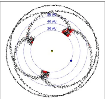
Figure 2shows the results of this simulation. Due to the (unrealistically) low libration amplitudes in this toy model simulation, the three resonant islands show up as discrete sets of orbits, with pericenters in three clusters: symmetric librators
6The inclinations are actually set to a very small value close to zero to avoid ambiguities in the other orbital angles.
FIGURE 2 | Black points show the positions of TNOs in a snapshot from this parametric toy model of TNOs in the 2:1 mean-motion resonance. The position of Neptune is shown by a blue circle, and dotted circles show distances from the Sun. Red points show simulated detections after running this model through the Survey Simulator. One third of the TNOs are in each libration island in the intrinsic model, but 2/3 of the detections are in the leading asymmetric island (having pericenters in the upper right quadrant of this plot). This bias is simply due to the longitudinal direction of pointings within the OSSOS ensemble and pericenter locations in this toy model of the 2:1 resonance.
are opposite Neptune, and leading and trailing are in the upper right and lower left of the plot, respectively7. While the intrinsic distributions in this model are evenly distributed among the three islands by design (33% in each), the detected TNOs are not. This is because TNOs on eccentric orbits are most likely to be detected close to pericenter, and in this toy model, the pericenters are highly clustered around three distinct positions on the sky8.
The red points in Figure 2 show the simulated TNOs that are detected by the OSSOS Survey Simulator. Just because of the positions of survey pointings on the sky, the detections are highly biased toward the leading island, which has over 2/3 of the detections, with fewer detections in the trailing island, and only 10% of all the detections in the symmetric island. Without knowing the on-sky detection biases (as is the case for TNOs pulled from the MPC database), one could easily (but erroneously) conclude that the leading island is much more
7We note that in reality the symmetric island generally has very large libration amplitudes and the pericenter positions of symmetric librators overlap with each of the asymmetric islands (e.g.,Volk et al., 2016), thus diagnosing the membership of each island is not as simple as this toy model makes it appear.
8While this is obviously an exaggerated example, pericenters in all of the resonant TNO populations are most likely to occur at certain sky positions, and thus this is an important consideration when discussing survey biases (seeGladman et al., 2012; Lawler and Gladman, 2013; Volk et al., 2016,for detailed discussions and analysis of these effects for resonant populations).
populated than the trailing island, when in fact the intrinsic populations are equal.
The relative fraction of n:1 TNOs that inhabit different resonant islands has been discussed in the literature as a diagnostic of Neptune’s past migration history (Chiang and Jordan, 2002; Murray-Clay and Chiang, 2005; Pike and Lawler, 2017). Past observational studies have relied on n:1 resonators from the MPC database with unknown biases, or the handful of n:1 resonators detected in well-characterized surveys to gain weak (but statistically tested) constraints on the relative populations. Upcoming detailed analysis using the full OSSOS survey and making use of the Survey Simulator will provide stronger constraints on this fraction, without worries about unknown observational biases (Chen, Y.-T., private communication).
3.3. Determining Intrinsic Population Size:
The Centaurs
The Survey Simulator can easily be used to determine intrinsic population sizes. As described in section 2.1, the Survey Simulator keeps track of the number of “drawn” simulated objects that are needed for the requested number of simulated tracked objects. By asking the Survey Simulator to produce the same number of tracked simulated objects as were tracked in a given survey, the number of drawn simulated objects is a realization of the intrinsic population required for the survey to have detected the actual number of TNOs that were found by the survey. By repeating this many times, with different random number seeds, different orbits and instantaneous positions are chosen from the model and slightly different numbers of simulated drawn objects are required each time. This allows us to measure the range of intrinsic population sizes needed to produce a given number of tracked, detected TNOs in a survey.
Here we measure the intrinsic population required to produce the 17 Centaurs that are detected in the OSSOS ensemble. Once the parameters of the orbital distribution and the H-distribution have been pinned down using the AD statistical analysis outlined in section 3.1 (this is done in detail for the Centaurs inLawler et al., 2018), we run the Survey Simulator until it produces 17 tracked Centaurs from the a < 30 AU portion of the Kaib et al. (2011) scattering TNO model, and record the number of simulated drawn objects required. As the OSSOS ensemble discovered Centaurs down to Hr ≃ 14, the Survey Simulator
is run to this H-magnitude limit. We repeat this 1,000 times to find the range of intrinsic population sizes that can produce 17 simulated tracked objects.
Using the properties of simulated objects in the drawn file, we measure the intrinsic population size to Hr < 12 (right
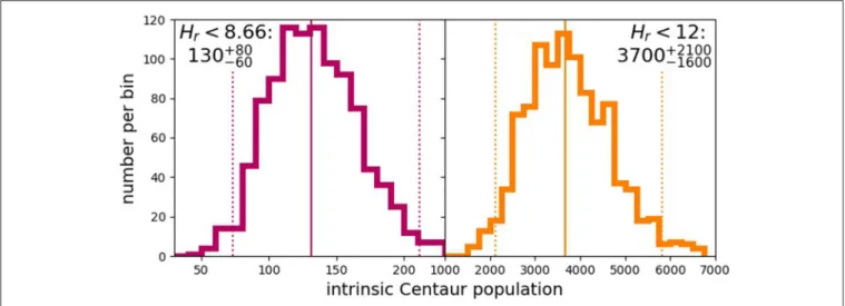
panel, Figure 3). The median intrinsic population required for 17 detections is 3700, with 97.5% of population estimates falling above 2100, and 97.5% falling below 5800 (these two values bracket 95% of the population estimates). The result is a statistically tested 95% confidence limit on the intrinsic Centaur population of 3700+2100−1600for Hr<12.
To ease comparison with other statistically produced intrinsic TNO population estimates (e.g.,Petit et al., 2011; Gladman et al.,
FIGURE 3 | The range of intrinsic Centaur population sizes required for the Survey Simulator to produce the same number of Centaur detections (17) as were discovered by the OSSOS ensemble, Hr<8.66 intrinsic populations shown in red (Left) and Hr<12 shown in orange (Right). The solid lines highlight the median population, and dotted lines show the 95% upper and lower confidence limits on the intrinsic Centaur population for each H-magnitude limit. Using the OSSOS ensemble, we measure an intrinsic populations of 130+80−60Hr<8.66 Centaurs and 3700+2100−1600Hr<12 Centaurs with 95% confidence.
2012), we also measure a population estimate for Hr < 8.66,
which corresponds to D & 100 km9 (left panel, Figure 3). Even though none of the detected Centaurs in OSSOS had Hr magnitudes this small, this estimate is valid because it is
calculated from our Survey Simulator-based population estimate and a measured H-magnitude distribution (from Lawler et al., 2018). For Hr<8.66, the statistically tested 95% confidence limit
on the intrinsic Centaur population is 130+80−60.
3.4. Constraints From Non-detections:
Testing a Theoretical Distant Population
Here we show a perhaps unintuitive aspect of the Survey Simulator: non-detections can be just as powerful as detections for constraining Kuiper Belt populations. Non-detections can only be used if the full pointing list from a survey is published along with the detected TNOs. An examination of the orbital distribution of TNOs in the MPC database makes it clear that there is a sharp dropoff in the density of TNO detections at a & 50 AU and q & 40 AU (Figure 2 inSheppard and Trujillo, 2016,
demonstrates this beautifully). Is this the result of observation bias or a real dropoff? Without carefully accounting for survey biases (Allen et al., 2001, 2002), by using the MPC database alone, there is no way to know.
Randomly drawing zero objects when you expect three has a probability of 5%, assuming Poisson statistics; thus, the simulated population required to produce three detections is the 95% confidence upper limit for a population that produced zero detections. As our example for non-detection upper limits, we create an artificial population in the distant, low-eccentricity Kuiper belt, where OSSOS has zero detections. Figure 4 shows
9The approximate H
rmagnitude that corresponds to D of 100 km is calculated assuming an albedo of 0.04 and using an average plutino color g − r = 0.5 (Alexandersen et al., 2016).
FIGURE 4 | Colored points show the relative populations and semimajor axis-eccentricity distributions from the CFEPS L7 model of the Kuiper belt, where absolute population estimates have been produced for each subpopulation in the well-characterized CFEPS survey (Petit et al., 2011; Gladman et al., 2012), populations are scaled to Hg<8.5 and color-coded by dynamical class. Resonances included in this model (those with >1 TNO detected by CFEPS) are labeled. A low-e artificial test population has been injected at 60 AU (black points); the number of points shows the upper limit on this population determined by zero detections in OSSOS, extrapolated to match the CFEPS model (Hr<8).
the CFEPS L7 debiased Kuiper belt10(Petit et al., 2011; Gladman
et al., 2012), where this low-eccentricity artificial population has been inserted at 60 AU (small black points) to demonstrate the power of non-detections, even in parameter space with low
sensitivity (i.e., low-e TNOs at 60 AU will never come very close to the Sun, thus will always remain faint and difficult to detect). We run this artificial population through the Survey Simulator until we have three detections in order to measure a 95% confidence upper limit on this population. At this large distance, we are only sensitive to relatively large TNOs (Hr . 7,
corresponding to D & 180 km for an albedo of 0.04). For there to be an expectation to detect three objects in the survey fields, the Survey Simulator tells us that there would need to exist a population of ∼90 such objects, which is our upper limit on this population. Extrapolating this population to match the H magnitude limits of the CFEPS L7 subpopulations plotted in
Figure 4, the total number of which are scaled appropriately for Hg < 8.5, gives ∼700 objects in this artificial population with
Hr<8.
This is a very small population size. We note that this specific analysis is only applicable to dynamically cold TNOs of relatively large size (Hr < 7). A steep size distribution could allow many
smaller TNOs to remain undiscovered on similar orbits. The point of this exercise it to show statistically tested constraints on populations with no survey detections. For comparison, at this absolute magnitude limit (Hr < 7), the scattering disk
is estimated to have an intrinsic population of ∼4000 (Lawler et al., 2018), the plutinos are estimated to have an intrinsic population of ∼500 (Volk et al., 2016), and the detached TNOs are estimated to number ∼4000 (Petit et al., 2011). Using the estimated populations and size distribution slopes from Petit et al. (2011)gives 3000 Hr<7 TNOs in the classical belt. The 3:1
mean-motion resonance, which is located at a similar semimajor axis (a = 62.6 AU), is estimated to have an Hr<7 population of
∼200 (Gladman et al., 2012). The 3:1 TNOs, however, are much more easily detected in a survey due to their higher eccentricities as compared with our artificial 60 AU population, thus a given survey would be sensitive to a larger H-magnitude for the 3:1 population than the 60 AU cold test population. This statistically tested population limit essentially shows that not very many low eccentricity, distant TNOs can be hiding from the OSSOS survey ensemble, especially when compared with other TNO populations.
4. CONCLUSION
Using TNO discoveries from well-characterized surveys and only analyzing the goodness of fit between models and TNO discoveries after forward-biasing the models gives a statistically powerful framework within which to validate dynamical models of Kuiper belt formation. Understanding the effects that various aspects of Neptune’s migration have on the detailed structure of the Kuiper belt not only provides constraints on the formation of Neptune and Kuiper belt planetesimals, but also provides useful comparison to extrasolar planetesimal belts (Matthews and Kavelaars, 2016). There are, of course, many lingering mysteries about the structure of the Kuiper belt, some of which may be solved by detailed dynamical simulations in combination with new TNO discoveries in the near future.
One such mystery is explaining the very large inclinations in the scattering disk (Shankman et al., 2016; Lawler et al., 2018) and inside mean-motion resonances (Gladman et al., 2012). Some possible dynamical mechanisms to raise inclinations include rogue planets/large mass TNOs (Gladman and Chan, 2006; Silsbee and Tremaine, 2018), interactions with a distant massive planet (Gomes et al., 2015; Lawler et al., 2017), and diffusion from the Oort cloud (Kaib et al., 2009; Brasser et al., 2012). These theories may also be related to the recent discovery that the mean plane of the distant Kuiper belt is warped (Volk and Malhotra, 2017).
Explaining the population of high pericenter TNOs (Sheppard and Trujillo, 2016; Shankman et al., 2017) is also difficult with current Neptune migration models. Theories to emplace high pericenter TNOs include dynamical diffusion (Bannister et al., 2017), dropouts from mean-motion resonances during grainy Neptune migration (Kaib and Sheppard, 2016; Nesvorný et al., 2016), dropouts from mean-motion resonances during Neptune’s orbital circularization phase (Pike and Lawler, 2017), interactions with a distant giant planet (Gomes et al., 2015; Batygin and Brown, 2016; Lawler et al., 2017), a stellar flyby (Morbidelli and Levison, 2004), capture from a passing star (Jílková et al., 2015), and perturbations in the Solar birth cluster (Brasser and Schwamb, 2015).
Here we have highlighted only a small number of the inconsistencies between models and real TNO orbital data. The level of detail that must be included in Neptune migration simulations has increased dramatically with the release of the full OSSOS dataset, containing hundreds of TNOs with the most precise orbits ever measured. The use of the Survey Simulator will be vital for testing future highly detailed dynamical emplacement simulations, and for solving the lingering mysteries in the observed structure of the Kuiper belt.
AUTHOR CONTRIBUTIONS
SL ran the simulations, created the figures, and wrote the majority of the text. JK wrote part of the text and helped plan simulations. BG, JK, and J-MP designed the OSSOS survey and proposed for telescope time. MB, JK, MA, BG, and J-MP took observations and reduced data for OSSOS. J-MP, JK, BG, CS, MA, MB, and SL helped write and test the Survey Simulator software and moving object pipeline.
FUNDING
SL gratefully acknowledges support from the NRC-Canada Plaskett Fellowship. MB is supported by UK STFC grant ST/L000709/1.
ACKNOWLEDGMENTS
The authors acknowledge the sacred nature of Maunakea, and appreciate the opportunity to observe from the mountain. CFHT is operated by the National Research Council (NRC) of Canada, the Institute National des Sciences de l’Universe of the Centre
National de la Recherche Scientifique (CNRS) of France, and the University of Hawaii, with OSSOS receiving additional access due to contributions from the Institute of Astronomy and Astrophysics, Academia Sinica, Taiwan. Data are produced and
hosted at the Canadian Astronomy Data Centre; processing and analysis were performed using computing and storage capacity provided by the Canadian Advanced Network For Astronomy Research (CANFAR).
REFERENCES
Adams, F. C. (2010). The birth environment of the solar system. ARAA 48, 47–85. doi: 10.1146/annurev-astro-081309-130830
Alexandersen, M., Gladman, B., Kavelaars, J. J., Petit, J.-M., Gwyn, S. D. J., Shankman, C. J., et al. (2016). A carefully characterized and tracked trans-neptunian survey: the size distribution of the Plutinos and the number of neptunian trojans. Astron. J. 152:111. doi: 10.3847/0004-6256/ 152/5/111
Allen, R. L., Bernstein, G. M., and Malhotra, R. (2001). The edge of the solar system. Astrophys. J. Lett. 549, L241–L244. doi: 10.1086/319165
Allen, R. L., Bernstein, G. M., and Malhotra, R. (2002). Observational limits on a distant cold Kuiper belt. Astron. J. 124, 2949–2954. doi: 10.1086/343773 Anderson, T. W. and Darling, D. A. (1954). A test of goodness of fit. J. Am. Stat.
Assoc. 49, 765–769. doi: 10.1080/01621459.1954.10501232
Bannister, M. T., Kavelaars, J. J., Petit, J.-M., Gladman, B. J., Gwyn, S. D. J., Chen, Y.-T., et al. (2016). The outer solar system origins survey. I. Design and first-quarter discoveries. Astron. J. 152:70. doi: 10.3847/0004-6256/152/3/70 Bannister, M. T., Shankman, C., Volk, K., Chen, Y.-T., Kaib, N., Gladman, B. J.,
et al. (2017). OSSOS. V. Diffusion in the orbit of a high-perihelion distant solar system object. Astron. J. 153, 262. doi: 10.3847/1538-3881/aa6db5
Bannister, M. T., Gladman, B. J., Kavelaars, J. J., Petit, J.-M., Volk, K., Chen, Y.-T., et al. (2018). OSSOS: VII. 800+ trans-Neptunian objects – The complete data release. APJS.
Batygin, K. and Brown, M. E. (2016). Evidence for a distant giant planet in the solar system. Astron. J. 151:22. doi: 10.3847/0004-6256/151/2/22
Batygin, K., Brown, M. E., and Betts, H. (2012). Instability-driven dynamical evolution model of a primordially five-planet outer solar system. Astrophys. J. Lett. 744:L3. doi: 10.1088/2041-8205/744/1/L3
Batygin, K., Brown, M. E., and Fraser, W. C. (2011). Retention of a primordial cold classical Kuiper belt in an instability-driven model of solar system formation. Astrophys. J. 738:13. doi: 10.1088/0004-637X/738/1/13
Bernstein, G. M., Trilling, D. E., Allen, R. L., Brown, M. E., Holman, M., and Malhotra, R. (2004). The size distribution of trans-Neptunian bodies. Astron. J. 128, 1364–1390. doi: 10.1086/422919
Brasser, R., Duncan, M. J., Levison, H. F., Schwamb, M. E., and Brown, M. E. (2012). Reassessing the formation of the inner Oort cloud in an embedded star cluster. Icarus 217, 1–19. doi: 10.1016/j.icarus.2011.10.012
Brasser, R. and Morbidelli, A. (2013). Oort cloud and scattered disc formation during a late dynamical instability in the solar system. Icarus 225, 40–49. doi: 10. 1016/j.icarus.2013.03.012
Brasser, R. and Schwamb, M. E. (2015). Re-assessing the formation of the inner Oort cloud in an embedded star cluster - II. Probing the inner edge. MNRAS 446, 3788–3796. doi: 10.1093/mnras/stu2374
Brown, M. E. (2017). Observational bias and the clustering of distant eccentric Kuiper belt objects. Astron. J. 154, 65. doi: 10.3847/1538-3881/aa79f4 Brunini, A. and Fernandez, J. A. (1996). Perturbations on an extended Kuiper disk
caused by passing stars and giant molecular clouds. Astron. Astrophys. 308, 988–994
Chiang, E. I. and Jordan, A. B. (2002). On the plutinos and twotinos of the Kuiper belt. Astron. J. 124, 3430–3444. doi: 10.1086/344605
Davis, D. R. and Farinella, P. (1997). Collisional evolution of edgeworth-kuiper belt objects. Icarus 125, 50–60. doi: 10.1006/icar.1996.5595
Dawson, R. I. and Murray-Clay, R. (2012). Neptune’s wild days: constraints from the eccentricity distribution of the classical Kuiper belt. Astrophys. J. 750:43. doi: 10.1088/0004-637X/750/1/43
Duncan, M., Quinn, T., and Tremaine, S. (1988). The origin of short-period comets. Astrophys. J. Lett. 328, L69–L73. doi: 10.1086/185162
Fernandez, J. A. (1980). On the existence of a comet belt beyond Neptune. MNRAS 192, 481–491. doi: 10.1093/mnras/192.3.481
Fraser, W., Alexandersen, M., Schwamb, M. E., Marsset, M., Pike, R. E., Kavelaars, J. J., et al. (2016). TRIPPy: Trailed Image Photometry in Python. Astron. J. 151:158. doi: 10.3847/0004-6256/151/6/158
Fraser, W. C., Bannister, M. T., Pike, R. E., Marsset, M., Schwamb, M. E., Kavelaars, J. J., et al. (2017). All planetesimals born near the Kuiper belt formed as binaries. Nat. Astron. 1:0088. doi: 10.1038/s41550-017-0088
Fraser, W. C., Brown, M. E., Morbidelli, A., Parker, A., and Batygin, K. (2014). The absolute magnitude distribution of Kuiper belt objects. Astrophys. J. 782:100. doi: 10.1088/0004-637X/782/2/100
Fraser, W. C. and Kavelaars, J. J. (2009). The size distribution of Kuiper belt objects for D gsim 10 km. Astron. J. 137, 72–82. doi: 10.1088/0004-6256/137/1/72 Gladman, B. and Chan, C. (2006). Production of the extended scattered disk by
rogue planets. Astrophys. J. Lett. 643, L135–L138. doi: 10.1086/505214 Gladman, B., Kavelaars, J. J., Nicholson, P. D., Loredo, T. J., and Burns, J. A.
(1998). Pencil-beam surveys for faint trans-Neptunian objects. Astron. J. 116, 2042–2054. doi: 10.1086/300573
Gladman, B., Lawler, S. M., Petit, J.-M., Kavelaars, J., Jones, R. L., Parker, J. W., et al. (2012). The resonant trans-Neptunian populations. Astron. J. 144:23. doi: 10. 1088/0004-6256/144/1/23
Gomes, R., Levison, H. F., Tsiganis, K., and Morbidelli, A. (2005). Origin of the cataclysmic late heavy bombardment period of the terrestrial planets. Nature 435, 466–469. doi: 10.1038/nature03676
Gomes, R. S., Soares, J. S., and Brasser, R. (2015). The observation of large semi-major axis Centaurs: testing for the signature of a planetary-mass solar companion. Icarus 258, 37–49. doi: 10.1016/j.icarus.2015.06.020
Hahn, J. M. and Malhotra, R. (2005). Neptune’s migration into a stirred-up Kuiper belt: a detailed comparison of simulations to observations. Astron. J. 130, 2392–2414. doi: 10.1086/452638
Hamid, S. E., Marsden, B. G., and Whipple, F. L. (1968). Influence of a comet belt beyond Neptune on the motions of periodic comets. Astron. J. 73, 727–729. doi: 10.1086/110685
Irwin, M., Tremaine, S., and Zytkow, A. N. (1995). A search for slow-moving objects and the luminosity function of the Kuiper belt. Astron. J. 110, 3082. doi: 10.1086/117749
Jewitt, D., and Luu, J. (1993). Discovery of the candidate Kuiper belt object 1992 QB1 Nature 362, 730–732. doi: 10.1038/362730a0
Jewitt, D. C. and Luu, J. X. (1995). The solar system beyond Neptune. Astron. J. 109, 1867–1876. doi: 10.1086/117413
Jílková, L., Portegies Zwart, S., Pijloo, T., and Hammer, M. (2015). How Sedna and family were captured in a close encounter with a solar sibling. MNRAS 453, 3157–3162. doi: 10.1093/mnras/stv1803
Jones, R. L., Gladman, B., Petit, J.-M., Rousselot, P., Mousis, O., Kavelaars, J. J., et al. (2006). The CFEPS Kuiper belt survey: strategy and presurvey results. Icarus 185, 508–522. doi: 10.1016/j.icarus.2006.07.024
Jones, R. L., Parker, J. W., Bieryla, A., Marsden, B. G., Gladman, B., Kavelaars, J., et al. (2010). Systematic biases in the observed distribution of Kuiper belt object orbits. Astron. J. 139, 2249–2257. doi: 10.1088/0004-6256/139/6/2249 Kaib, N. A., Becker, A. C., Jones, R. L., Puckett, A. W., Bizyaev, D., Dilday, B.,
et al. (2009). 2006 SQ372: A likely long-period comet from the inner Oort cloud. Astrophys. J. 695, 268–275. doi: 10.1088/0004-637X/695/1/268
Kaib, N. A., Roškar, R., and Quinn, T. (2011). Sedna and the Oort cloud around a migrating Sun. Icarus 215, 491–507. doi: 10.1016/j.icarus.2011.07.037 Kaib, N. A. and Sheppard, S. S. (2016). Tracking Neptune‘s migration history
through high-perihelion resonant trans-Neptunian objects. Astron. J. 152:133. doi: 10.3847/0004-6256/152/5/133
Kavelaars, J., Jones, L., Gladman, B., Parker, J. W., and Petit, J.-M. (2008a). The orbital and Spatial Distribution of the Kuiper Belt (Tucson, AZ: University of Arizona Press).
Kavelaars, J. J., Gladman, B., Petit, J., Parker, J. W., and Jones, L. (2008b). “The CFEPS High Ecliptic Latitude Extension,” in AAS/Division for Planetary
Sciences Meeting Abstracts #40 (Ithaca, NY: Bulletin of the American Astronomical Society), 481.
Kavelaars, J. J., Jones, R. L., Gladman, B. J., Petit, J., Parker, J. W., Van Laerhoven, C., et al. (2009). The Canada-France ecliptic plane survey L3 data release: the orbital structure of the Kuiper belt. Astron. J. 137, 4917–4935. doi: 10.1088/ 0004-6256/137/6/4917
Kobayashi, H. and Ida, S. (2001). The effects of a stellar encounter on a planetesimal disk. Icarus 153, 416–429. doi: 10.1006/icar.2001.6700
Lawler, S. M. and Gladman, B. (2013). Plutino detection biases, including the kozai resonance. Astron. J. 146:6. doi: 10.1088/0004-6256/146/1/6
Lawler, S. M., Shankman, C., Kaib, N., Bannister, M. T., Gladman, B., and Kavelaars, J. J. (2017). Observational signatures of a massive distant planet on the scattering disk. Astron. J. 153:33. doi: 10.3847/1538-3881/153/1/33 Lawler, S. M., Shankman, C., Kavelaars, J.,Alexandersen, M., Bannister, M. T.,
Chen, Y.-T., et al. (2018). OSSOS. VIII. The transition between two size distribution slopes in the scattering disk. Astron. J. 155, 197. doi: 10.3847/1538-3881/aab8ff
Levison, H. F., Morbidelli, A., Van Laerhoven, C., Gomes, R., and Tsiganis, K. (2008). Origin of the structure of the Kuiper belt during a dynamical instability in the orbits of Uranus and Neptune. Icarus 196, 258–273. doi: 10.1016/j.icarus. 2007.11.035
Lykawka, P. S. and Mukai, T. (2008). An outer planet beyond Pluto and the origin of the trans-Neptunian belt architecture. Astron. J. 135, 1161–1200. doi: 10. 1088/0004-6256/135/4/1161
Malhotra, R. (1993). The origin of Pluto’s peculiar orbit. Nature 365, 819–821. doi: 10.1038/365819a0
Malhotra, R. (1995). The origin of Pluto’s orbit: implications for the solar system beyond Neptune. Astron. J. 110, 420. doi: 10.1086/117532
Matthews, B. C. and Kavelaars, J. (2016). Insights into planet formation from debris disks: I. The solar system as an archetype for planetesimal evolution. SSR 205, 213–230. doi: 10.1007/s11214-016-0249-0
Morbidelli, A., Gaspar, H. S., and Nesvorny, D. (2014). Origin of the peculiar eccentricity distribution of the inner cold Kuiper belt. Icarus 232, 81–87. doi: 10. 1016/j.icarus.2013.12.023
Morbidelli, A. and Levison, H. F. (2004). Scenarios for the origin of the orbits of the trans-Neptunian objects 2000 CR105and 2003 VB12(Sedna). Astron. J. 128, 2564–2576. doi: 10.1086/424617
Murray-Clay, R. A. and Chiang, E. I. (2005). A signature of planetary migration: the origin of asymmetric capture in the 2:1 resonance. Astrophys. J. 619, 623–638. doi: 10.1086/426425
Nesvorný, D. (2015a). Evidence for slow migration of Neptune from the inclination distribution of Kuiper belt objects. Astron. J. 150:73. doi: 10.1088/0004-6256/ 150/3/73
Nesvorný, D. (2015b). Jumping Neptune can explain the Kuiper belt kernel. Astron. J. 150:68. doi: 10.1088/0004-6256/150/3/68
Nesvorný, D. and Vokrouhlický, D. (2016). Neptune’s orbital migration was grainy, not smooth. Astrophys. J. 825:94. doi: 10.3847/0004-637X/825/2/94 Nesvorný, D., Vokrouhlický, D., and Morbidelli, A. (2013). Capture of trojans by
jumping Jupiter. Astrophys. J. 768:45. doi: 10.1088/0004-637X/768/1/45 Nesvorný, D., Vokrouhlický, D., and Roig, F. (2016). The orbital distribution of
trans-Neptunian objects beyond 50 au. Astrophys. J. Lett. 827:L35. doi: 10.3847/ 2041-8205/827/2/L35
Parker, A. H. (2015). The intrinsic Neptune Trojan orbit distribution: implications for the primordial disk and planet migration. Icarus 247, 112–125. doi: 10.1016/ j.icarus.2014.09.043
Parker, A. H. and Kavelaars, J. J. (2010). Destruction of binary minor planets during Neptune scattering. Astrophys. J. Lett. 722, L204–L208. doi: 10.1088/ 2041-8205/722/2/L204
Petit, J., Kavelaars, J. J., Gladman, B., Jones, R. L., Parker, J. W., Van Laerhoven, C., et al. (2011). The Canada-France ecliptic plane survey - Full data release: the orbital structure of the Kuiper belt. Astron. J. 142:131. doi: 10.1088/0004-6256/142/4/131
Petit, J.-M., Holman, M., Scholl, H., Kavelaars, J., and Gladman, B. (2004). A highly automated moving object detection package. MNRAS 347, 471–480. doi: 10. 1111/j.1365-2966.2004.07217.x
Petit, J.-M., Kavelaars, J. J., Gladman, B. J., Jones, R. L., Parker, J. W., Bieryla, A., et al. (2017). The Canada-France Ecliptic Plane Survey (CFEPS)—high-latitude component. Astron. J. 153, 236. doi: 10.3847/1538-3881/aa6aa5
Petit, J.-M., Morbidelli, A., and Valsecchi, G. B. (1999). Large scattered planetesimals and the excitation of the small body belts. Icarus 141, 367–387. doi: 10.1006/icar.1999.6166
Pike, R. E., Kavelaars, J. J., Petit, J. M., Gladman, B. J., Alexandersen, M.,d Volk, K., et al. (2015). The 5:1 Neptune resonance as probed by CFEPS: dynamics and population. Astron. J. 149:202. doi: 10.1088/0004-6256/ 149/6/202
Pike, R. E. and Lawler, S. (2017). Details of resonant structures within a nice model Kuiper belt: predictions for high-perihelion TNO detections. Astron. J. 153, 127. doi: 10.3847/1538-3881/aa5be9
Pike, R. E., Lawler, S., Brasser, R., Shankman, C. J., Alexandersen, M., and Kavelaars, J. J. (2017). The structure of the distant Kuiper belt in a nice model scenario. arXiv:1701.07041v1
Schwamb, M. E., Brown, M. E., and Rabinowitz, D. L. (2009). A search for distant solar system bodies in the region of Sedna. Astrophys. J. Lett. 694, L45–L48. doi: 10.1088/0004-637X/694/1/L45
Schwamb, M. E., Brown, M. E., Rabinowitz, D. L. and Ragozzine, D. (2010). Properties of the distant Kuiper belt: results from the palomar distant solar system survey. Astrophys. J. 720, 1691–1707. doi: 10.1088/0004-637X/720/2/ 1691
Shankman, C., Kavelaars, J., Gladman, B. J., Alexandersen, M., Kaib, N., Petit, J.-M., et al. (2016). OSSOS. II. A sharp transition in the absolute magnitude distribution of the Kuiper belt‘s scattering population. Astron. J. 151:31. doi: 10. 3847/0004-6256/151/2/31
Shankman, C., Kavelaars, J. J., Bannister, M. T., Gladman, B. J., Lawler, S. M., Chen, Y.-T., et al. (2017). OSSOS. VI. Striking biases in the detection of large semimajor axis trans-Neptunian objects. Astron. J. 154, 50. doi: 10.3847/1538-3881/aa7aed
Sheppard, S. S. and Trujillo, C. (2016). New extreme trans-Neptunian objects: toward a super-earth in the outer solar system. Astron. J. 152:221. doi: 10.3847/ 1538-3881/152/6/221
Silsbee, K. and Tremaine, S. (2018). Producing distant planets by mutual scattering of planetary embryos. Astron. J. 155:75. doi: 10.3847/1538-3881/ aaa19b
Stern, S. A. (1995). Collisional time scales in the Kuiper disk and their implications. Astron. J. 110, 856. doi: 10.1086/117568
Stern, S. A. (1996). Signatures of collisions in the Kuiper disk. Astron. Astrophys. 310, 999–1010
Thommes, E. W., Duncan, M. J., and Levison, H. F. (1999). The formation of Uranus and Neptune in the Jupiter-Saturn region of the solar system. Nature 402, 635–638. doi: 10.1038/45185
Trujillo, C. A., Jewitt, D. C., and Luu, J. X. (2001). Properties of the trans-Neptunian Belt: statistics from the Canada-France-Hawaii telescope survey. Astron. J. 122, 457–473. doi: 10.1086/321117
Trujillo, C. A. and Sheppard, S. S. (2014). A Sedna-like body with a perihelion of 80 astronomical units. Nature 507, 471–474. doi: 10.1038/nature 13156
Tsiganis, K., Gomes, R., Morbidelli, A., and Levison, H. F. (2005). Origin of the orbital architecture of the giant planets of the Solar System. Nature 435, 459–461. doi: 10.1038/nature03539
Volk, K. and Malhotra, R. (2017). The curiously warped mean plane of the Kuiper belt. Astron. J. 154, 62. doi: 10.3847/1538-3881/aa79ff
Volk, K., Murray-Clay, R., Gladman, B., Lawler, S., Bannister, M. T., Kavelaars, J. J., et al. (2016). OSSOS III—Resonant trans-Neptunian populations: constraints from the first quarter of the outer solar system origins survey. Astron. J. 152:23. doi: 10.3847/0004-6256/152/1/23
Conflict of Interest Statement: The authors declare that the research was
conducted in the absence of any commercial or financial relationships that could be construed as a potential conflict of interest.
Copyright © 2018 Lawler, Kavelaars, Alexandersen, Bannister, Gladman, Petit and Shankman. This is an open-access article distributed under the terms of the Creative Commons Attribution License (CC BY). The use, distribution or reproduction in other forums is permitted, provided the original author(s) and the copyright owner are credited and that the original publication in this journal is cited, in accordance with accepted academic practice. No use, distribution or reproduction is permitted which does not comply with these terms.