Dynamic stiffness and seismic response of pile groups

DYNAMIC STIFFNESS AND SEISMIC RESPONSE OF PILE GROUPS

AMIR MASSOUD YYNIA / B.S., U n i v e r s i t y o f Tehran (1 977) M. S.

,

Massachusetts I n s t i t u t e o f Technology (1 979) Submitted i n p a r t i a l f u l f i l l m e n t o f t h e requirements f o r t h e degree o f Doctor o f Philosophy a t t h e

MASSACHUSETTS INSTITUTE OF TECHNOLOGY January 1982

@ Massachusetts I n s t i t u t e o f Technology, 1982

. -

.-

-

Signature o f Author

. . .

6 r .

. . .

Department o f C i v i 1 Engineering, January 22, 1982

. . .

. . .

C e r t i f i e d b y .

. . .

-7

~ d u a r d o ~ y e l , Thesis Supervisor

Acceptedby

. . .

Chairman, Departmental Committee on Graduate Stu- dents o f the- Department o f C i v i l Engineering.

M'g'~E%EiVdLI#~ViTUTE

ABSTRACT

DYNAMIC STIFFNESS AND SEISMIC RESPONSE OF PILE GROUPS by

AMIR MASSOUD KAYNIA

Submitted to the Department of Civil Engineering in January 1982 in partial fulfillmentof the requirements for the degree of

Doctor of Philosophy

A formulation for the analysis of pile groups in layered semi-infinite media is presented. The formulation was based on the intro-duction of a soil flexibility matrix as well as on dynamic stiffness and flexibility matrices of the piles, in order to relate the dis-cretized uniform forces to the corresponding displacements at the pile-soil interface.

The result of pile group analyses showed that the pile group behavior is _{highly frequency-dependent as the result of wave} inter-ferences taking place between the various piles in the group. Large values for stiffnesses as well as large magnification factors for the force on certain piles is.expected at some frequencies. As for the seismic response, pile groups essentially follow the low-frequency components of the ground motion, and the rotational component is negli-gible for typical dimensions of the foundation.

A numerical study on the accuracy of the approximate superposition method as well as the quasi-three-dimensional formulation, in which the pile-soil compatibility conditions are accounted for in the formulation only in the direction of vibration, showed that these solutions compare very well with the full three-dimensional solution.

Thesis Supervisor: Eduardo Kausel

Associate Professor of Civil Engineering

Acknowledgements

I would like to express my deep gratitude to my advisor, professor Eduardo Kausel, for his invaluable guidance and enthusi-asm during the thesis research.

I am greatly indebted to professors John M. Biggs, Robert V. Whitman, and Jerome J. Connor, members of my doctoral thesis com-mittee, for their many constructive suggestions and their interest in this work.

Sincere thanks also go to Mrs. Jessica Malinofsky for her ex-ceptional care and patience in typing this thesis.

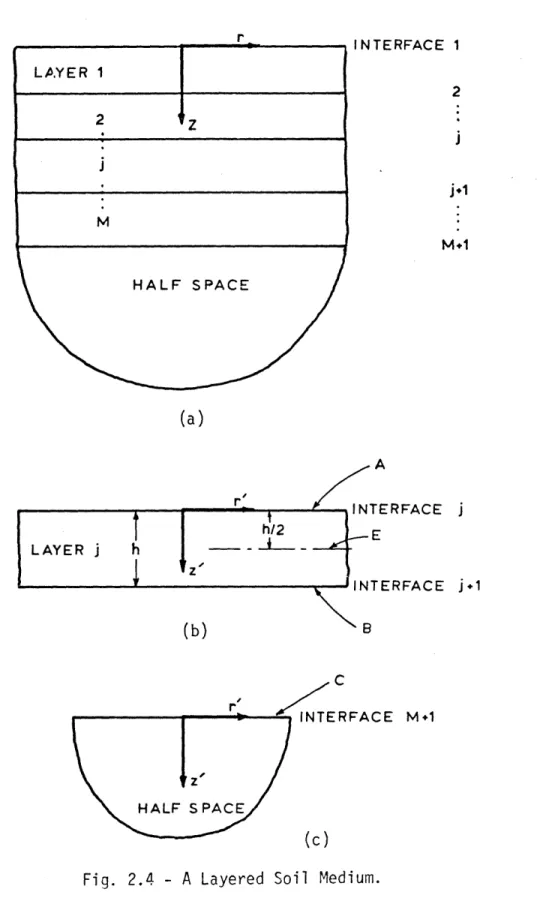
Table of Contents Abstract 2 Acknowledgements 3 Table of Contents 4 List of Figures 5 List of Symbols 8 1 - INTRODUCTION 11

2 - FORMULATION AND ANALYTICAL DERIVATIONS 15

2.1 - Formulation 15

2.2 - Response of Viscoelastic Layered Soil Media to 26 Dynamic Stress Distributions

2.2.1 - Solution of the equations of motion 27 2.2.2 - Layer and halfspace stiffness matrices 35 2.2.3 - Displacements within a layer 46 2.2.4 - Integral representation and numerical 49

evaluation of displacements

2.3 - Lateral and Axial Vibration of Prismatic Members 63

2.3.1 - Lateral vibration 63

2.3.2 - Axial vibration 68

3 - DYNAMIC BEHAVIOR OF PILE GROUPS 72

3.1 - Dynamic Stiffnesses of Pile Groups ₇₆

3.2 - Seismic Response of Pile Groups ₉₀

3.3 - Distribution of Loads in Pile Groups ₉₄

4 - THREE-DIMENSIONAL VS. QUASI-THREE-DIMENSIONAL SOLUTIONS 102

5 - THE SUPERPOSITION METHOD 111

6 - SUMMARY AND CONCLUSIONS 123

List of Figures Title

Distribution of Forces on the jth Pile of the Group. Forces on the Pile and in the Free-field.

The Type of Loads in the Soil Medium. A Layered Soil Medium.

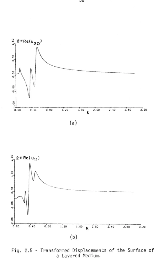
Transformed Displacements of the Surface of a Layered Medium.

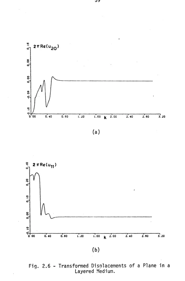
Transformed Displacements of a Plane in a Layered Medium.

A Beam in the Lateral Vibration. A Beam in the Axial Vibration.

Pdage 16 23 28 38 56 59 64 69 2.1 2.2 2.3 2.4 2.5 2.6 2.7 2.8 3.1 3.2 3.3 3.4 3.5 3.6 3.7 3.8 3.9 Figure No.

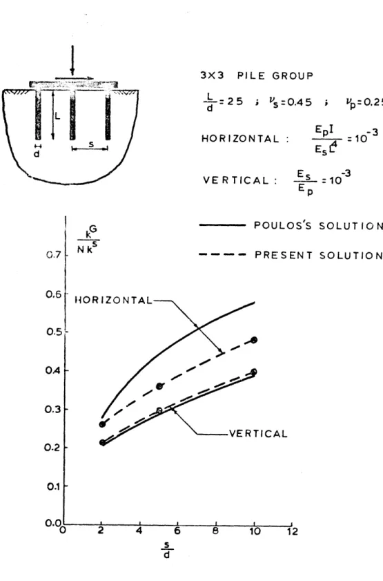
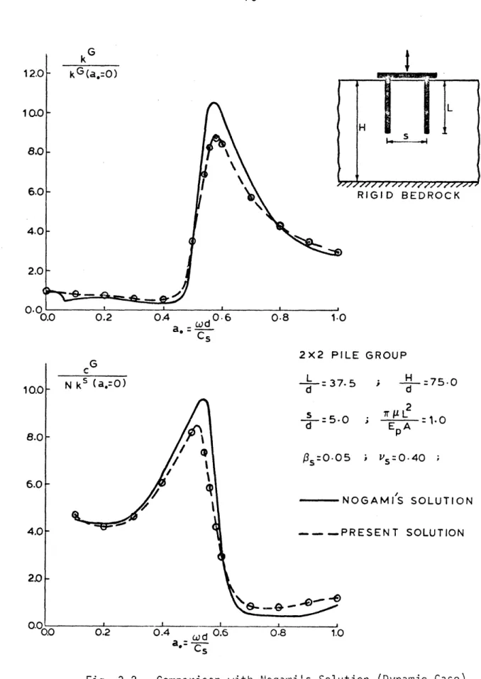
Comparison with Poulos's Solution (Static Case). 74 Comparison with Nogami's Solution (Dynamic Case). 75 Horizontal and Vertical Dynamic Stiffnesses of 2 x 2 78 Pile Groups in a Soft Soil Medium.

Horizontal and Vertical Dynamic Stiffnesses of 3 x 3 80 Pile Groups in a Soft Soil Medium.

Horizontal and Vertical Dynamic Stiffnesses of 4 x 4 81 Pile Groups in a Soft Soil Medium.

Horizontal and Vertical Dynamic Stiffnesses of 3 x 3 82 Pile Groups in a Soft Soil Medium (Hinged-Head Piles).

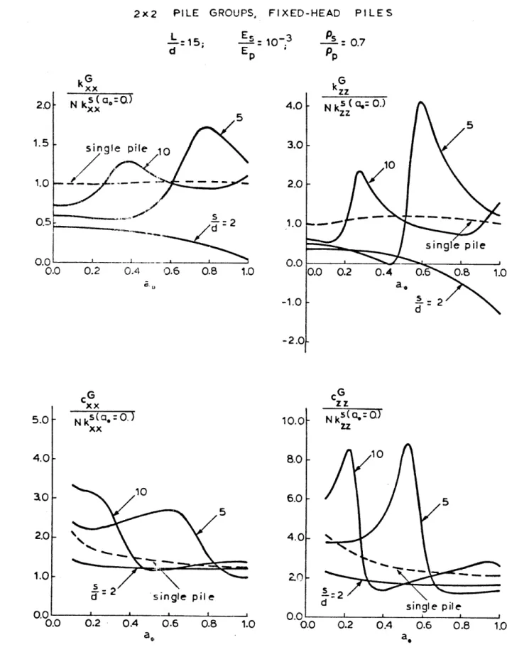
Horizontal and Vertical Dynamic Stiffnesses of Pile 83 Groups with s/d = 5 in a Stiff Soil Medium.

Rocking and Torsional Dynamic Stiffnesses of 2 x 2 85 Pile Groups in a Soft Soil Medium.

Rocking and Torsional Dynamic Stiffnesses of 3 x 3 86 Pile Groups in a Soft Soil Medium.

Title

Rocking and Torsional Dynamic Stiffnesses of 4 x 4 Pile Groups in a Soft Soil Medium.

Rocking and Torsional Dynamic Stiffnesses of 3 x 3 Pile Groups in a Soft Soil Medium (Hinged-Head Piles). Rocking and Torsional Dynamic Stiffnesses of Pile Groups with s/d = 5 in a Stiff Soil Medium.

Effect of a Near Surface Soft Soil Layer on the Stiff-ness of Pile Groups and Single Piles.

3.10 3.11 3.12 3.13 3.14 3.15 Absolute Value of tal Displacement Pile Groups in a Transfer Functions and Rotation of the Soft Soil Medium.

Page

for the Horizon-Pile Cap for 2 x for the Horizon-Pile Cap for 3 x for the Horizon-Pile Cap for 4 x Absolute Value of Transfer Functions for the Horizon-tal Displacement and Rotation of the Pile Cap for 3 x Pile Groups in a Soft Soil Medium (Hinged-Head Piles). Absolute Value of Transfer Functions for the Horizon-tal Displacement and Rotation of the Pile Cap for Pile Groups with s/d = 5 in a Stiff Soil Medium.

Distribution of Horizontal Pile Groups in a Soft Soil

and Vertical Medium. Distribution of Horizontal and Vertical Pile Groups in a Soft Soil Medium.

Forces in 3 x 3 Forces in 4 x 4 Distribution of Horizontal and Vertical Forces in 3 x 3 Pile Groups in a Soft Soil Medium (Hinged-Head Piles). Horizontal and Vertical Dynamic Stiffnesses of 4 x 4 Pile Groups in a Soft Soil Medium by the Quasi-Three-Dimensional Formulation.

Horizontal and Vertical Dynamic Stiffnesses of Pile Groups with s/d = 5 in a Stiff Soil Medium by the Quasi-Three-Dimensional Formulation.

Figure

No.

Absolute Value of Transfer Functions tal Displacement and Rotation of the Pile Groups in a Soft Soil Medium. Absolute Value of Transfer Functions tal Displacement and Rotation of the Pile Groups in a Soft Soil Medium. 3.16 3.17 3.18 3.19 3.20 3.21 4.1 4.2 100 101 104 105

Figure Title Page No.

4.3 Rocking and Torsional Dynamic Stif-fnesses of 4 x 4 Pile 107 Groups in a Soft Soil Medium by the Quasi-Three-Dimensional

Formulation.

4.4 Rocking and Torsional Dynamic Stiffnesses of Pile Groups 108 with s/d = 5 in a Stiff Soil Medium by the

Quasi-Three-Dimensional Formulation.

4.5 Absolute Value of Transfer Functions for the Horizontal 109 Displacement and Rotation of the Pile Cap for 4 x 4 Pile

Groups in a Soft Soil Medium by the Quasi-Three-Dimensional Formulation.

4.6 Absolute Value of Transfer Functions for the Horizontal 109 Displacement and Rotation of the Pile Cap for Pile Groups

with s/d-= 5 in a Stiff Soil Medium by the Quasi-Three-Dimensional Formulation.

5.1 Interaction Curves for the Horizontal and Vertical Dis- 113 placement of Pile 2 due to the Horizontal and Vertical

Forces on Pile 1.

5.2 Interaction Curves for the Rotation of Pile 2 due to the 114 Horizontal Force and Moment on Pile 1.

5.3 Forces and Displacements at the Head of Two Piles. 115 5.4 Horizontal and Vertical Dynamic Stiffnesses of 4 x 4 Pile 118

Groups in a Soft Soil Medium by the Superposition Method.

5.5 Rocking and Torsional Dynamic Stiffnesses of 4 x 4 Pile 119 Groups in a Soft Soil Medium by the Superposition Method.

5.6 Horizontal and Vertical Dynamic Stiffnesses of Pile Groups 120 with s/d = 5 in a Stiff Soil Medium by the Superposition

Method.

5.7 Rocking and Torsional Dynamic Stiffnesses of Pile Groups 121 with s/d = 5 in a Stiff Soil Medium by the Superposition

List of Symbols ao A p Cxx' CZZ_' c¢ ,c Cs d Ep and _E s fr' f0' fz frn' fens fzn fIn' f2n' f3n F

Fp

F_s h H i Ip Fuxx' F _uzFz} uxx _IxMx Jn(kr) k kxx, kzz, nondimensional frequency

area of the pile cross section

dampings of the foundation (pile group) associated with horizontal, vertical, rocking and torsional modes of vibration

shear wave velocity of the soil medium diameter of the piles

moduli of elasticity of the piles and of the soil

body forces in the soil medium in the r, e, and z direc-tions

amplitudes of Fourier sine or cosine series of fr' f and f

combinations of Hankel transforms of f rn fen and fzn axial force in a beam (pile)

dynamic flexibility matrix of fixed-end piles dynamic soil flexibility matrix

thickness of a layer

constant axial force in a beam (pile) =

-T

moment of inertia of the pile cross section

interaction factors

nth order Bessel function of the 1st kind

parameter of a Hankel transfor

stiffnesses of the foundation (pile groups) associated with horizontal, vertical, rocking and torsional modes

List of Sym•bols (Continued) K K L m M N px, P Pe P* r R R_x t Ug ux, Urs Urn Uln'u2n'u3n Ue

combinations of Hankel transforms of urn, en and uzn vector of displacements of the pile-soil interface vector of displacements of the pile ends

dynamic stiffness of the foundation (pile group) dynamic stiffness matrix of the piles

no. of segments along the pile length length of the piles

mass per unit length of the piles moment at a pile section

total no. of piles in a group

Py' P forces developed at the pile-soil interface in the x, y, and z directions

vector of forces developed at pile-soil interface vector of forces at pile ends

vector of free-field forces distance in the radial direction

radius of the piles

R y Rz forces (reactions) at the pile ends in the x, y and z

directions

distance (spacing) between adjacent piles time

free-field ground-surface displacement

U y uz .displacements of the pile-soil interface in the x, y and

z directions

u , uz displacements in the soil medium in the r, 0 and z

direc-6 ations

List of Symbols (Continued) U* V a Bp, B._ps Y A TI n

S,9

Up and , s pp and _ps arz S.a

_ez

_oZZ arzn _{9'Ozn' zzn} a_{2 1}

_{n' U22n}

_'0

2 3n

vector of free-field displacements shear at a pile section

a parameter defined for the soil medium (eq. (2.46)) material dampings in the piles and in the soil

a parameter defined for the soil medium (eq. (2.47))

dilatation (eq. (2.23))

a pE ireter defined for the piles (eq. (2.143)) a pa -eter defined for the piles (eq. (2.132)) anog. t.etween a vertical plane and the x-z plane

La-me constants

PoiT_: -n ratios of the piles and the soil

a parameter defined for the piles (eq. (2.132)) mass densities of the piles and the soil

stresses on a horizontal plane

amplitudes of Fourier sine or cosine series of arz, aez

and azz

combinations of Hankel transforms of arzn_{, aOzn and azzn} rotation of the pile cap

rotations of the pile cross section

dynamic flexibility matrix of the piles for end displace-ments

frequency of steady-state vibration.

Also the superscripts "G" and "s" were used to refer to the quan-tities in the pile group and in the single pile, respectively.

CHAPTER 1 - INTRODUCTION

A pile is a structural element installed in the ground which is connected to the structural frame, either directly or through a founda-tion block, in order to transfer the loads from the superstructure to the ground. Piles are seldom used singly; more often, they are used in

groups or clusters, in which case they are connected to a common founda-tion block (pile cap).

Pile four~datiois, under certain circumstances, are preferred over shallow founda..ions; for instance, in sites where near-surface soil strata are so weak that either soil properties do not have the required strength, or the settlement and/or movements of a shallow footing on such ground would be intolera.ble.

Behavior of pile foundations, sometimes referred to as deep founda-tions, has been a subject of considerable research. Most studies have focussed primarily on short- and long-term static pile behavior, pile-installation effects, estimation of ultimate load capacity and settlement, prediction of ultimate lateral resistance, and estimation of lateral

deflection. Extensive field testings and experimental investigations on different aspects of pile behavior have resulted in a number of empir-ical and approximate analytempir-ical methods for the pile-foundation design. In addition, other studies have resulted in more rigorous schemes for pile analysis. Among these studies the works of Poulos (1968), Poulos and Mattes (1971), Poulos (1971), Butterfield and Banerjee (1971) and Banerjee (1978) are related to the present study. These researchers dis-cretized the piles into several segments and related the displacements of the segments to the corresponding forces in both the soil medium, using

Mindlin's fundamental solution (1936) and in the piles, using pile dif-ferential equations (in discretized form). Introduction of the condition of displacement compatibility between the soil and the piles and imposi-tion of appropriate boundary condiimposi-tions lead to the desired pile soluimposi-tion. The results of these studies, especially by Poulos and his colleagues, have hfghlighted the important aspects of static pile-group behavior,

in-cluding: distribution of loads among the piles in a group, stiffnesses of pile groups, and tihe variation of these quantities with geometric param-eters (spacin9, lei.gzh, and number of piles) as well as material

proper-ties. For a comprehensive review of these results and other analytical and empirical techniques of static pile-foundation analysis see Poulos

(1980).

The fact that -s.atic pile behavior studies were unable to provide any qualitative infor;ration on dynamic aspects of the problem, along with an increasing demand for the construction of nuclear power plants and off-shore structures, have stimulated extensive research on dynamic pile be-havior.. For these studies, which have dealt primarily with the behavior of single piles, a variety of different models and solution schemes have

been used. Tajimi (1969), Nogami and Novak (1976), Novak and Nogami (1977), Kobori, Minai and Baba (1977, 1981). Kagawa and Kraft (1981)

have obtained analytical solutions for the response of dynamically-excited single piles. Finite-element techniques, on the other hand, have been used byl Blaney, Kausel and Roesset (1975) and Kuhlemeyer (1979a, 1979b). In additifon, less involved models based on the theory of beams on elastic foundations, commonly referred to as the subgrade-reaction approach, were used by Novak (197421, Matlock (1970),Reese, Cox and Koop (1974) and Reese and Welch (1975). The advantage of this technique is that the results

of field testing can be directly incorporated in the model ("p-y" and

"t-w" techniques).

In spite of considerable achievements in characterizing the dynamic response of single piles, the dynamic behavior of pile groups is not yet well understood. In fact, only a few attempts have been made to study

this problem. The earlier contributions are due to Wolf and Von Arx

(1978), and to Nogami (1979). Wolf and Von Arx used an axisymmetric finite-element schene to obtain Green functions for ring loads which were used to form the soil flexibility matrix. The dynamic stiffness matrix of the pile-soil syst:m wa: then obtained by simply assembling those of the soil and piles. Using tiis formulation, Wolf and Von Arx studied some charac-teristics of horizontal as well as vertical dynamic stiffnesses of pile groups in a layered soil stratum resting on a rigid bedrock. Later this methodology was employed by Waas and Hartmann (1981), who implemented an

efficient and rigorous technique for the computation of the Green's func-tions (Waas, 1980), to study the behavior of pile groups in lateral vibra-tion.

On the other hand, the vertical vibration characteristics of pile groups in a uniform soil stratum underlain by a rigid bedrock has been studied analytically by Nogami (1979). To incorporate in his model the interaction of piles through the soil medium, Nogami used an analytical solution to the axisymmetric vibration of the stratum obtained earlier by Nogami and Novak (1976). Later he extended his studies to the case of layered: strata (Nogami, 1980). For this case, however, the interaction effects were obtained using an analytical expression for the displacement field due to the ax-al vibration of an infinitely long rigid cylinder in an infinite. m5dium ('Iovak, Nogami and Aboul-Ella, 1978).

The results of these studies indicate that: 1) behavior of pile groups is strongly frequency-dependent; 2) spacing and number of piles have a considerable effect on dynamic stiffnesses, but only a minor ef-fect on the lateral seismic response; and 3) interaction efef-fects are stronger for more flexible soil media.

The objective of the present work is to study the three-dimensional dynamic behavior of pile groups in layered semi-infinite media and to

investigate the accuracy of certain approximate approaches. Chapter 2 of this report is cevoted to the formulation and the associated

analyt-ical derivations. In Chapter 3 the results of the three-dimensional analyses are prese'nted. These results include dynamic stiffnesses and

seismic response of pile groups as well as the distribution of loads among the piles in the group. Special attention is paid to the effect

of frequency, spacing, and number of piles on these quantities. In Chap-ter 4 the accuracy of a "quasi three-dimensional" solution is investi-gated (a quasi three-dimensional solution here refers to the solution obtained for symmetric rectangular arrangement of piles by assuming that the dynamic effects in the vertical and in the two horizontal directions of symmetry are uncoupled from one another).

The applicability of the superposition scheme to dynamic pile-group analysis is examined in Chapter 5. In addition, the characteristics of dynamic interaction curves (the influence of vibration of one pile on another for a group of two piles) and their connection to pile-group

be-havior are studied.

Finally, Chapter 6 includes a summary of the important aspects of the pile-group behalior as well as conclusions on the applicability of approximate solutiion schemes.

CHAPTER 2 - FORMULATION AND ANALYTICAL

LERIVATIONS

In the present study it is assumed that 1) the soil medium is a viscoelastic layered halfspace, 2) the piles are made of linear elastic materials, and 3) there is no loss of bondage between the piles and the soil; however, the frictional effects due to torsion and bending of piles are neglected. (The overall pile group behavior is controlled primarily by the frictional and lateral forces caused by axial motion and bending of the piles, respectively.)

In what follows, the formulation of the problem,along with the associ-ated analytical derivations and their numerical implementation, are pre-sented. _{Any time-de3endent variable such as u(t) used in this formulation} is of the form u(t) = _{u exp (iOt), in which u is a complex quantity, w is} the frequency of st3ady-state harmonic vibration, and i = V-T. However,

the factor exp (iwt) is deleted in the equations, since it is shared by all time-dependent variables involved in the problem.

2.1 Formulation

Con'sider the pile group shown in Fig. 2.1. The actual distribution of lateral as well as frictional forces developed at the pile-soil inter-face are. shown for one of the piles in the group (pile j).

The pile is discretized into k arbitrary segments, and the pile-tip is _{considered to be segment (z+l). The pile head and the center of the} pile segments define then (z+2) "nodes" ,,hich are assigned numbers 0, 1, 2, ... , (+1), respectively. Subsequently, the actual force distributions are replaced by piecewise constant distributions which are also shown in the figure. These :forces are assumed positive if they are in the positive

actual distributio of lateral forces

in the y-direction

Fiq. 2.1 - Distribution of Forces on the jth Pile of the Group

Consider first the equilibrium of pile j under the pile-soil interface forces. If one denotes the vector of the resultant of these forces by PJ, that is:

PJ =[P

x

P

_{ly lz...(+l)x (+l)y P(Il)}

P 3 i + + T

T

(2.1) and the vector of displacements of nodes 1 through (+1l) by Uj, that is:

U=[ u j Uj U u U (2.2)

lx ly uz ... u (+l)x (+l)y u (+l)z

Then Uj can be expressed as the summation of the displacements caused by the translations and rotations of the two pile ends when there are no loads on the pile, and the displacements caused by forces on the piles

(-PJ) when the two ends of the pile are clamped. This can be expressed as:

U3 TO UJ - F PJ (2.3)

e p

in which UJ is the vector of end displacements for pile j, given by: e

e [U o x u z u (' ( ](.

J is a (3(t+l)x 10) matrix defining displacements of the center of seg-ments (nodes 1 through (£+1) due to end displaceseg-ments of the pile when PJ are not present (to be more specific, the ith column of -J defines the

three components of translation at the center of the segments due to a unit harmonic pile end displacement associated with the it h component of

Uj), and F is the flexibility matrix of pile j associated with nodes 1

through ( ), for the fixed-end codition. (Since the ends of the pile through (Z+l), for the fixed-end condition. (Since the ends of the pile

are fixed, the entries in FJ corresponding to node (f+1) are zero.) p

If, in addition, one denotes the dynamic stiffness matrix of pile j by Kj , and the vector of external forces and moments at the two ends of this pile by PJ, that is

P=[R I M R J J Rj Rj _{R R I}j

Ri+ T

e = [Rx ox o oy oy oz R(+l)x M(+l)x (Z+l)y (Z3+l)y R(Z+l)zT (2.5) Then one can write

P= _e KjUj _+U jT1 pj (2.6)

p e

The first term in Eq. (2.6) corresponds to pile-end forces due to pile-end displacements (U ) when there are no loads on the pile, and the second term corresponds to pile-end forces due to loads on the pile (-PJ) when the two ends of the pile are fixed. Since the forces at the pile

tips are included in Pi and matrices FJ and yj are constructed such that p

they contain the effects of forces and displacements at this point, one

has to set R+l)x R+l)y and R3 _{+l)z equal to-zero. In addition, for}

floating piles M+l)x and M+)y are taken to be zero as well.

Defining now the global load and displacement vectors for the N piles in the group:

Se

p2

U e I

Se e (2.7)

K1 p P K-p K N p

0

F p 1 'P \ * FN P "N

One can then write the following equations for the ensemble of piles in the group (compare with eqns. (2.3) and (2.6)):

U = U e - Fp P

Pe = Kp Ue + T P

(2.9)

Consider next the equilibrium of the soil mass under forces P (dis-tributed uniformly over each segment; see Fig. 2.1). If Fs denotes the

flexibility matrix of the soil medium, relating piecewise-constant seg-mental loads to the average displacements along the segments, then

U . Fs P

(2.8)

Finally combining eqns. (2.9) and (2.10) one getsi

P= [Kp + T (F_s + F )l ee K Ue (2.11)

Ke is a (10N x 10N) matrix which relates only the five components of forces at each end of the piles to their corresponding displacements. In other words, the degrees of freedom along the pile length have been con-densed out without forming a complete stiffness matrix. It is also impor-tant to notice that in the solution of eq. (2.11) it is not necessary to invert (Fs + F p) as indicated; instead, one only needs to perform a

triangular decomposition of this matrix.

Matrix Ke relates forces and displacements at the pile ends in a group of unrestrained piles. In order to obtain dynamic stiffnesses of a rigid foundation (pile cap) to which the piles are connected, one needs to impose the appropriate geometric (kinematic) and force boundary condi-tions at the pile heads and pile tips. (The boundary condicondi-tions at pile tips, as discussed earlier, are zero forces at these points for floating piles.) At pile heads, on the other hand, the boundary conditions are in general a combination of geometric and force conditions, unless all the piles are rigidly connected to the foundation, in which case only geome-tric conditions should be considered. Once the pile head forces for the possible modes of vibration (horizontal, vertical, rocking and torsional) are computed, dynamic stiffnesses of the foundation at a prescribed point are obtained b.- simply calculating, in each mode, the resultant of these forces at the prescribed point.

To extend the formulation to seismic analysis, one only needs to express the displacements U as the summation of seismic displacements

in _{the medium when the piles are.removed (i.e., soil with cavities)}

_U,

and the displacements caused by pile-soil interface forces P, that is:

U = U + F_s P (2.12)

Combination of eqns. (2.8) and (2.12) results in

Pe = [Kp + T (F

s

+ Fp)l l] Ue - T (F

s

+ Fp)-l

Y

(2.13)

or

Pe = Ke Ue + P-e (2.14)

where Ke (as in eq. (2.11)) is the dynamic stiffness for the ensemble of piles associated with the degrees of freedom at pile heads and pile tips, and P = - (F + F)l p defines consistent fictitious forces at these points which reproduce the seismic effects.

In order to calculate the response of the rigid foundation to which the piles are connected, one has to impose the necessary geometric and force boundary conditions. (The procedure is similar to that described for the calculation of foundation stiffnesses, except that for the seis-mic case one has to use the fact that the resultant of pile-head forces on the foundation is zero.)

From the development of the preceding formulation it is clear that

Fs is the flexibility of a soil mass which results from the removal of

the piles; in other words, Fs corresponds to the soil mass with N cavi-ties. Similarly, _{U refers to the seismic displacements in} the medium with the cavities. Due to the fact that evaluation of the same quanti-ties in a uniform soil mass, in which the cavities have been filled with

the soil, requires much less computational effort than the original problem, it is very desirable to modify the formulation in order to make use of this numerical efficiency. The following discussion pertains to such a modification.

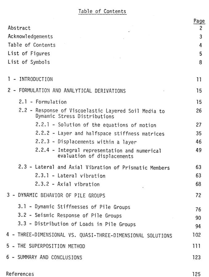
Consider the semi-infinite soil medium and the pile shown in Fig. 2.2a. It is assumed that p(z) and u(z) define lateral soil pressure and lateral pile displacement, respectively. (For convenience, only one pile and one type of force at the pile-soil interface are considered. The modi-fication procedure, however, is independent of the number of piles and the type of interaction force.) For a pile element shown in Fig. 2.2b, one can write the equilibrium equation as:

dV + p Aw 2u = p _(2.15)

in which A and Pp denote the cross-sectional area and mass density of the pile, respectively.

Next, consider the same soil medium except that the pile is removed and the resulting cavity is filled with soil such that the original uni-form soil mass (before the installation of the pile) is obtained. The dashed line in Fig. 2.2c shows the periphery of the added soil column. Further, suppose that f(z) defines a force distribution along the height of the soil column which causes approximately the same displacement u(z) at the centerline of this soil column. Now consider the equilibrium of forces on a soil differential element shown in Fig. 2.2d. (The vertical sides of this element extend just beyond the dashed line); one can then write:

-p

(a)

(b) fdr1

dz

_I 2 -PsAw udz

(c)

(d)

Fig. 2.2 - Forces on the Pile and in the Free Field.

pd z

,i M

Z

where p' is the lateral force on the element. This equation implies that one can remove the soil column and apply the distributed force pi on the cavity's wall to preserve the equilibrium of the soil mass. (This is clearly an approximate scheme, since the effects of frictional forces due to the lateral displacement of the soil column are neglected.)

If one takes p' to be equal to p, eq. (2.16) can be rewritten as

dV' + p A 2_u + f ₌ p _(2.17)

Thus the displacement u(z) due to a distributed force p(z) in the soil mass with the cavity can be reproduced by the application of the distri-buted force f(z) to the uniform (no cavity) soil medium. f(z) is given by:

f = p - A 2 u _{- dV}

(2.18)

Similarly, the equilibrium of the differential pile element can be ex-pressed in terms of the distributed force f; introducing eq. (2.17) into eq. (2.15), one gets:

-d (V-V') + (p - Ps)A2u f (2.19)

Eq. (2.19) can be interpreted as the differential equation of a beam with a mass density (Pp - Ps) and a modulus of elasticity (Ep - Es) and

sub-jected to a distributed force f(z). (Es is the elasticity modulus of

the soil.)

The approximate scheme presented here suggests that if one replaces P in eqns. (2.9) and (2.10) by the vectorial equivalent of the distributed forces f (say, F), then the soil flexibility matrix Fs should be taken

as that corresponding to a uniform (no cavity) soil mass and the matri-ces Kp, Fp and T corresponding to piles with reduced mass density and elasticity modulus (obtained by subtracting the mass density and elas-ticity modulus of the soil from the corresponding quantities of the piles). The final expression relating pile-head forces with displace-ments is then of the same form as that given by eq. (2.11), except that Fs corresponds to a soil without cavities, and Kp, Fp, ' to piles with

reduced properties.

A similar modification applies to the seismic analysis. In addition, the seismic displacements in the soil mass with the cavities (U in eq. 2.12)) can be related to the associated free-field (no cavity) seismic displacements. If the free-field displacements are denoted by U* and the corresponding free-field forces are denoted by P*, then one can write: (since P = 0):

U = U - F P (2.20)

However, the effect of free-field forces, in most pile-soil interaction problems, can be neglected. Therefore one might approximate U by U in the formulation of the seismic problem.

In what follows a numerical technique to evaluate a soil flexibility matrix is presented, and expressions for the elements of Kp, Fp and ' are derived.

2.2 Response of Viscoelastic Layered Soil Media to Dynamic Stress Distributions

The formulation presented in Sec. 2.1 requires the evaluation of a dynamic flexibility matrix, Fs , for the soil medium. This matrix

de-fines a relationship between piecewise-uniform loads distributed over cylindrical or circular surfaces (corresponding to pile shafts and pile tips) and the average displacement of these regions. Although there are a number of ways to obtain a value to represent the displacement of a loaded region, the weighted averaging, originally proposed by Arnold, Bycroft and Warburton (1955), is believed to provide the most meaningful displacement value. In order to understand the basis for the weighted average displacement, consider the response of a medium to a set of distributed loads q', q2, .. .. acting on regions D1, D2 .... , respec-tively. Suppose a virtual displacement v(x,y,z) is introduced in the medium. If the component of this displacement in the direction of qi is denoted by vi(x,y,z), then the virtual work done by the total dynamic force Qi D= i q dA is given by:

Qi. := = i qi vi dA (2.21)

where vi is the weighted average virtual displacement in region Di.

Equa-tion (2.21) shows that, on the basis of the work done by the total force, the weighted average displacement is the most appropriate quantity to represent the displacement field. For uniformly distributed loads, as eq. (2.21) indicates, the weighted average displacementis identical to the average displacement in the region.

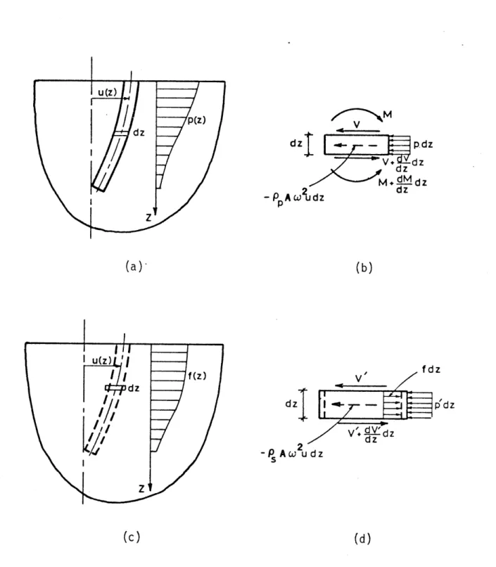
The objective of this section is to present details of a numerical technique which enables one to compute displacements caused by loads uniformly distributed over cylindrical or circular surfaces in layered viscoelastic soil media. The types of load involved in the problem are shown in Fig. 2.3; the loads on cylindrical surfaces are associated with stresses on pile shaft and those on circular surfaces correspond to pile tip stresses.

The method used here for response calculation is similar to that presented by Apsel (1980). For the present work, however, the stiffness approach, based on assemblage of layer stiffness matrices, is used. 2.2.1 - Solution of the equations of motion

If ur , ue and uz are the displacements in the radial, tangential,

and vertical directions, and fr' fe and fz are the associated external loads per unit volume, the equations of motion of an elastic body in cylindrical coordinates are:

(+2) TWz + 2p 1-+w 2_{pu + f =0} a r

a

I+ r r Sr 8z 2 (X+2u) 1 A 2p + 21 +r +w pU + f = _{0 (2.22)} r

a

az ae (2.22) (x+2p) 3 - 2P (rm) + 211 mr 2 2 z r

ar

r

e

+ pu_z + fz =

where X and p are Lame's constant, p is the mass density, and w is the frequency of steady-state vibration; the dilatation A and the rotations Wr' m and q are given by:

U

4

4q44J~

a) uniform horizontal load

on cylindrical surface

b) uniform vertical load on cylindrical surface

R

c) uniform horizontal load on circular surface,

d) uniform vertical load on circular surface

Fig. 2.3 - The Type of Loads in the Soil Mledium.

A -1 a (ru ) + 1 e a+ r Dr r r Be az =1 1 Uz u8 S(rue)

a

-(2,23) (2.24)

For a viscoelastic medium with an internal energy dissipative be-havior of the iyster*etic type, one only needs to replace X and 'P in Eqns.

(2.22) by the compl.:x Lame moduli given by:

Ic = X(l _{+ 2Bi)}

c

_{= P(l}

₊

2Bi)

where a is commonly referred to as the fraction of critical damping. The first step in the solution of Eqns. (2.22) is to separate variables. This can be achieved by expanding displacements and body forces in a Fourier series in tangential direction, that is

(2.25) ur (r, ,z)

Uo

(r,o,z)

uz (r, ,z) fr (r, ,z) fr, (r, ,z) fz (r, 8,z)

Z=

Urn n=O 0o = U

an

n=O

S

Y

uz

Uzn n=O Co n=O rn n=O I

X

zn n=O (r,z) cos nO (r,z) sin nO (r,z) cos nO (r,z) cos nO (r,z) sin nO (r,z) cos ne (2.26)

Introduction of these expansions, along with Eqns. (2.23) and (2.24), into Eqns. (2.22) leads to

= a u ₂ au ₂ 2 a _a 2U₂ r +rn 1 3Urn n + 1 ] + n=O r 2 r ar r2 rn az ar ar r az -2 n + + 2P U + f}rn cos ne = 0 (2.27) 2 2 00n _{0 +} aUoen n2+1 _{u +} 2un _{_+!_} n - (,+,j) n VL r ar 2 un 2 n = ar r az

-2, n urn + m2pn + fen sin ne = 0 (2.28)

2U2 a2U { 2z[ u

₊

1 auzn n2

_U

₊

2 zznAn

2

]

_{+ (X+)}

n=0 ar r

az

+ 2p Uzn + fzn cos ne = 0 (2.29) where au 1 (ru) + n + azn (2.30) Ln r ar rn r

en

z

In order that Eqns. (2.27), (2.28) and (2.29) be satisfied, it is necessary that the terms in accolades be identically zero. If, in addi-tion, one combines the two equations resulting from (2.27) and (2.28), then the following three conditions, to be satified for any value of n, are obtained: 2 _{2 2} P[-- (urn u )+e + (u +u )- (n +u rn+ ( U )] 2 rn en r ar rn

en

r2 Urn On 2 rn ar r2 ae + ( ) ( nn) + p (Urn + Uen) + (frn + f ) = 0 (2.31)

__5r-

T(rn

n

+

en

rn

on

2

2 (u - u ) +1

a

(u - u ) - (n-1 ) (u

2

- u ₎₊

_a

2

2 ( u _-n ) ] 2 l rn an r ar (urn n 2 rn nen 2 rn un

ar

r az + (x+[) [-• _3r +- n] _{r n} + 2p (u_rn 2 a2u iau C[-.•n + zn ar 2 n -• Uzn r - u _on ) + f r n _irn- fn ) = 0 2 + a z ]+ n I ) a + 2p uzn az + fzn (2.32) = 0 (2.33)

If now the following Hankel Transforms are defined

Uln (k,z) + U3n (k,z) = - Uln (k,z) + u3 n (k,z) U2n (k,z) = fln (k,z) + f3n (k,z) - fin (k,z) + f3n (k,z) fo (urn )o

= (urn

f

00₀

=

0

(

rn

=

(f rn

0 + Uon) Jn+l - Uen) Jn-(kr) rdr (kr) rdr uzn Jn (kr) rdr_znn (2.34) + fen ) Jn+1 (kr) rdr rdr fzn Jn (kr) rdr

where J (kr) is the nth order Bessel function of the 1st kind, and if

the following identities are used,

1

2

2

₂

_d

2

₂

[ + r r]q + Jmr(kr ) rdr= (J- k) m(kr) rdr Sar r Ra dz o (2.35) f2n (k,z) - f n) Jn-I (kr)

dr rm

T

m

(kr) rdr

o

( + _{m) Jm} (kr) rdr : k Jm (kr) rdr

Tr- r

fO

Then one can show that application of (2.32) and (2.33) leads to:

2 - -d- _ k 2 + 2 a] (u1 + ) + (X+2 2 dz _d • _k2 _{2 -uln+u}1 n 3n 3n)+ (X+ d2 - k2 2 ] u2n dz I dz

)(-k

p)(k

n+

where

f

f0

An J

n

(kr)

rdr is

the nth

Using Eqns. (2.36) and (2.37) and the fol tions,

n J (kr) = + -d- J (kr) r n shodr n one dan show that

= ku, + --- u n -In dz 2n

kel Transforms to Eqns. (2.31),

An) + fln + f3n = 0 (2.38)

An) n + f3n = 0 (2.39)

f2n = 0 (2.40)

order Hankel Transform of An.

lowing property of Bessel

func-+ k Jn+l (kr) (2.41)

(2.42) Finally, if one introduces Eq. (2.42) into Eqns. (2.38) - (2.40), and Eqns. (2.38) and (2.39) are combined (by adding and subtracting them), the following ordinary differential equations are obtained:

(2.36)

(2.37)

d2 [p

-

k2 (X+2p) +pw 2 Uln dz -(1+) k u2n + fn = ₀

2

(+) k uln + [(d+2 ) 2 Pk2 2] U2n + 2n = 0 dz 2 d 2 2 ( dz2 P- k + p ) u3n + f3n = 0 dz (2.43) (2.44)

(2.45)

Equations (2.43) and (2.44) define a system of two ordinary linear dif-ferential equations for uln and U2n. U3n, on the other hand, is un-coupled from uln and u2n and can be obtained by solving Eq. (2.45).

It is convenient at this point to introduce the following two parameters:

cx

= k2 pw2 S +2\

a 2p

=- k2 2

C2 :

=

_{k2 - ry}

where Cs and Cp are the velocities of shear waves and pressure waves,

respectively. (For viscoelastic materials Cs and Cp are complex

quanti-ties). Introduction of these parameters into Eqns. (2.43), (2.44) and (2.45) leads to: (x+') k -uln +d 2 2 u2n 2n + fin= 0 = 0 (2.48a) (2.48b) d2 2 ( 2 - y ) U3n

+

f3n = 0 dz (2.49)

In _{order to obtain the homogenous solution of Eqns. (2.48), one} can take uln = Aenz _{and U2n = Be}z _{and substitute in Eqns. (2.48). The}

(2.46) (2.47)

• V

resulting system of algebraic equations for n and A/B yields four sets of solutions, which can be used to define the general homogeneous solu-tions for uln and U2n. Following this procedure, one obtains:

e z H k C

e

+k1 z y

uH

(k,z) =

-

kCln e +C

2

n

e

-

kC

3

neaz +yC

4

n

ez

uH (k,z) = - aC e z + k C e- z + C ez - kC eYz 2n ln 2n 3n 4n

(2.50)

where C1n(k), C2n(k), C(k)k) and C4n(k) are unknown constants. To

ob-tain a particular solution one can use the method of variation of parameters; however, for the loadings involved in the present problem, fln and f2n' as will be shown in section 2.2.4, are independent of z; therefore particular solutions can be obtained by inspection. One such set of solutions for uln and u2n are:

Finally, the solutions

P 1 Un= 2 a ( +2 .) u2n 7 f2n of Eqns. (2.48) fln (2.51)

are given by:

Cln e- O

l n

(k

_z)

_-kY

_-k

_{C2n e-YZ}

_fn/2

_(Xf

₊₂₎

(2 52)

Uln _(2.52)

u2n (k,z) L -a k a -k1 C3n e f2n

C4n eYZ

A similar procedure applied to Eq. (2.49) leads to the solution of this equation:

C e-YZ 1 C5n

e

u (k,z) = [ 1 1] eY +n fy (2.53)

3n

C

6ey

2

3n

3

2

2.2.2 - Layer and halfspace stiffness matrices

In order to determine the unknown constants in Eqns. (2.52) and (2.53) it is necessary to use the appropriate kinematic and force boundary conditions of the problem. Since Eqns. (2.52) and (2.53) ex-press displacements in the transformed space, it is necessary to derive expressions for the associated transformed stresses.

The three components of stress on a plane perpendicular to the z-axis in cylindrical coordinates are given by:

rz _z az_r

au 1 au

Cz = (- + r ) (2.54)

auz

ozz

=

2- +

xz

If the Fourier expansion of u_{r ,} u₀ and uz , given by Eq. (2.26),

are used in the above equations, one gets

0o

arz Z arzn cosnO n=O Co = C 8zn sin ne z n sin no (2.55) a = zzn cos no n=O

where orzn, a0 zn and ozzn are given by rn = a( Uzn rzn ar

+ -au

az 0_{z =( aUen n n)} ezn 5z r zn S =

azn

rzzn = _{2 , az} + XA

and An is given by Eq.

By combining Eqns.

(2.30).

(2.56) and (2.57) and reordering Eq. (2.58), one can write: + auzn rzn ezn ar arzn

n

a(

+ n

)]

r Uzn z rn Uen +n +n(u r zn az rn - Uon)] azn z = (X+2-) z

zzn

az

+x(ar

Urn rn

r

_+n

nr

₎

ar r r

en

If the following Hankel Transforms are defined,

+ a2 3n(k,z)

=

To

+ 02 3n(k,z) =

(arz _{n +} )ezn) _{Jn+l(kr) rdr}

(crzn - Oezn) Jn- (kr) rdr (2.60)

0_zzn J_{n (kr) rdr}

Then Hankel transforms of Eqns.

(2.56) (2.57) (2.58) (2.59) o21n(k, z ) •021 n(k,z) a2 2n(k,z) auzn a zn

ezn

= [arzn

Jr

f

o

(2.59) leads to:

- a t o =

[ k + d

+

21n

' "23n L- 2n dz Uln T U3n

- 21n + a2 3n =I [ku2n + ýz (- Uln + U3n)] (2.61) du

2 2n = (X+2p) -n + (kuln)

I, 22n ý ....

Finally by using the expressions obtained for uln, U2n, and U3n (Eqns. (2.52) and (2.53)), one can express the transformed stresses c21n a23n' arnd C2 2 n as:

Cln e

a 21n(k,z) rk 2 -(k2 + 2 ) -2ak (k2+y2) C2n e-Yz

S22n(k,z) :L Y2 ) -2Yk (k2 2 ) -2fk C 3n e C4 n eYZ + kf2n/Y (2.62) Xkf _In/a2 (X+2p)

SC5ne

z

a₂₃n(k,z) =i [-Y Y] Yz (2.63)

6n eYZJ

At this point it is convenient to distinguish between the solutions corresponding to uln and u2n and those corresponding to u3n. Since the solution of u3n involves only Y, all quantities associated with u3n will be identified as "SH-wave" quantities. In a similar manner, "SV-P waves" will be used to refer to quantities associated with uln and U2n.

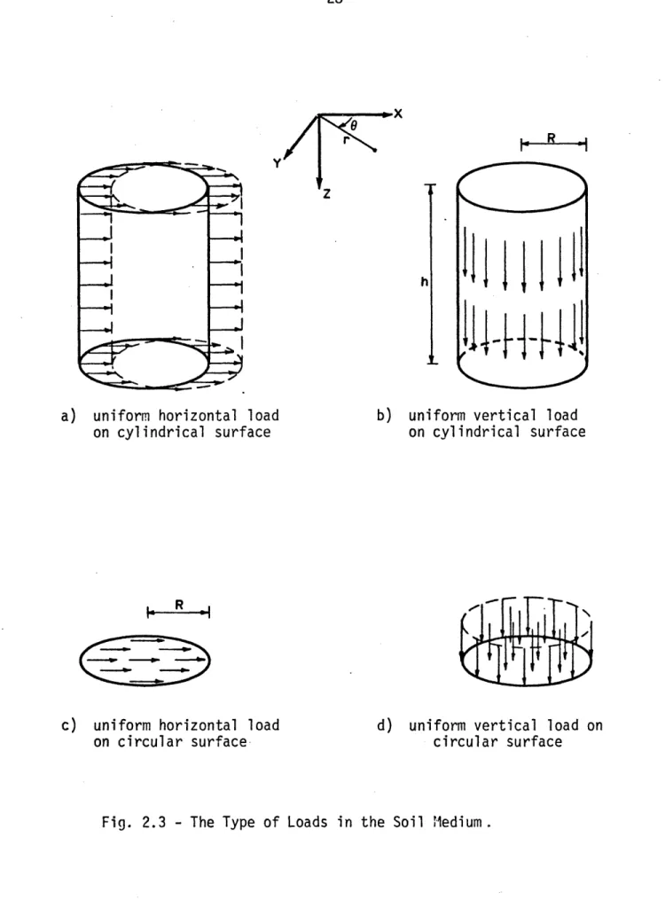
Consider the layered soil medium shown in Fig. 2.4a. The medium consists of M layer: resting on a halfspace. Fig. 2.4b shows the jth

INTERFACE 1 2

jM+1

M+I (a) RFACE j RFACE j+1 C r

(c)

Fig. 2.4 - A Layered Soil Medium.

J_

k U)

INTERFACE M+1

z

_*

layer confined between the two planes denoted by A and B, and Fig. 2.4c shows the halfspace bounded by the plane C. The objective is now to obtain a relationship between the transformed stresses on the two planes A and B in Fig. 2.4b and the transformed displacements of these planes. Such a relationship can be used to define layer "stiffness matrices" as well as layer "fixed-end stresses." In a similar manner,

a relationship between stresses and displacements for plane C in Fig. 2.4c results in halfspace stiffness matrices. For a given value of k, the stiffness matrices of the layers and the halfspace and the associ-ated force vectors can be used to assemble the stiffness matrix and the load vector for the layered medium; the resulting system of equa-tions then yields the transformed displacements uln, U2n and u3n at layer interfaces.

Layer stiffness matrix and load vector for SV-P waves

For the layer shown in Fig. 2.4b, one can use Eq. (2.52) to obtain the expressions for the transformed displacements uln and u2n of the two planes A and B associated with local coordinates z' = 0, and z' = h; the result can be written in matrix form as

A Uln - Uln

A

uA

_2n

u

_2n

uB -n u

_{2n u2n)}

u -k y -k y -a k a -k

-ke--ah ye-h keCah yeYh

-ae -ah ke-yh cae.h -keYh

C n C2 n (2.64) C3n 4 n

-where uln and u2n are given by:

u fln-/ a (X+2! l)

U2n _{= f2n/Y} P

Similarly, Eq. (2.62) can be used to express the transformed stresses

0_{21n and c22n on the exterior side of planes A and B} as:

A

₁

0_{21n a21n}

A +

-

i

022n +22n, B c21n -21n a22n - '22n = I -2ak (k2 + 2) -(k2+y2) 2Yk tke - a_{h -(k}2 _{2 )eyh}

Sk2+2)e

- a

_h

_-2Yke-y

h

where a21n and a2 2n are given by:

2ak -(k2 ₊ 2₎ -(k2 +y2) 2Yk - 2akeah (k2+ 2_)eYh (k2 +y 2)eh -2YkeYh c21n = -kf2n a22n = ~kfn/a2 (X+21p)

Finally a relationship between the transformed stresses (o21n and c22n) on planes A and B and the transformed displacements (Uln and U2n) of these planes can be obtained by deleting the unknown constants C1n,

C2n, C3n and C4n between Eqns. (2.64) and (2.67). The result can be

written in the form

AB

"iCiSV

=

[KA

_plV

_{_P]}

]

_SV

{

uABr

₀

₊

_{CSV _}

-AB

(2.70)

(2.65)

(2.66) In C 2n . C_3n C_4n (2.67) (2.68) (2.69)

AB AB

where

{

_{SV-P and usvP}

displacement vectors, that is

denote the transformed stress and

[-AA

3AB_.

is

the vector

A a21 n A a22n B 02 1 n B 022n A un uAp} uAn u _ P U2n B u U.₁ n B U2n

of "fixed-end stresses" given by

(-AB = -KAB

I SV-P

sv-f

Uln u2n Uln u2n

- 21n

-

22n '.21n '22n (2.72)

and the elements of the symmetric 4 x 4 layer stiffness matrix [KAB_ are given by the following expressions: (AB and SV-P are omitted.)

K11 = - p (k-2 2) [aySCY - k2 YCa]

K21 D pk [cy(3k2+ )(CY - 1) (k4 + k 2 + 2_{u2 y2) SaSY]}

K₃₁ = pi(k - y 2) [k2S - cySO1

K_{4 1} pkay(k2 - y2) [CY - Ci ]

K₂₂ =TY(k2 _{_ y}2_{) [ ySYCa - k}2_Sa

_CY

K32 =- K_{4 1}

K42 - y(k2 -y2) [k2Sc - cySY] K_{3 3 = K} 11 K43 =- K21 K44 = K22 (2.73) In these expressions D =ay[-2k2 + 2k2CC - a2 + k4 SaSY] (2.74) and Ca,

C6

S: and :Y are used to denote the following quantities:

Ca cosh(-h) ; S - sinh(ah)

(2.75) CY _ cosh(vh) S

Y _{= sinh(yh)}

For the case ii which -k--s<< T, one might use the asymptotic

values of these expressions to avoid loss of significant digits in the operations (in fact for m=O the above stiffness terms become indefinite; i.e., zero divided by zero). For this case, one can show that

2 K11 ~ D- k[kh(l-_2) - (1+s2) Skck] K21 ~~~ k[k2h2(-E2)2 _{_} 2(1+E2)(Sk)2] K31 ~2 ~- k[(l+E2)Sk - kh(l-c2)Ck] D

K

41

--

-

-2

k[kh(1-E

2

)Sk]

D K₂₂ ~_ _D Uk[kh(l-c ) + (l+E2) skck]

K42 ~ - 1k[(l+E2)Sk + kh(l-E 2)Ck] (2.76) D

where

D=k2h2(1-~2) - (+:2) 2(Sk)2 . (2.77)

S= Cs /C and Ck and Sk denote the following quantities

Ck cosh (kh) ; Sk sinh(kh) (2.78)

Halfspace stiffness matrix for SV-P waves

To evaluate transformed displacements and stresses in a halfspace, one can use Eqns. (2.52) and (2.62) provided that, for the forced-vibration problems, the radiation conditions are satisfied. That is, as z approaches inF-inity, the value of stresses and displacements should tend to zero. This requires that the unknown constants C3n and C4n in

Eqns. (2.52) and (2.62) be set equal to zero. (The real part of a and y is positive). Thus, for the halfspace shown in Fig. 2.4c, one can write the following expressions for the transformed displacements and stresses at plane C (surface of the halfspace) associated with the local coordin-ate z = 0; (fln = _f2n = ₀₎

Sn

(2.79)

SC21n

I

-(k2

2)

_2Yk

_Cn(2.80)

22n 2Y Kn

C

Kcj{

Ulnf

KSV-

U C

a2n

where the symmetric 2 x 2 halfspace stiffness matrix is given by:

[K C ₁₁ LKSV-PJ

_{k -ay}

ar

(k

2

_{- y}

2

₎

k(k 2 _{+ y 2 2c y}

₎

2 2

k(k +y - 2ay) y(k2 2 (2.82)

y(k

-

)J

and for the case in

which

I

-<<

1_

by

and for the case in which Il-FU-<< 1 by

[KCSV-P]

2k-2

+

1+e 2C

21

(2.83)

and E = Cs/C

Layer stiffness matrix and load vector for SH waves

Following the procedure described for SV-P waves, one can use Eqns. (2.53) and (2.63) to express transformed displacements and external stresses associated with planes A and B in Fig. 2.4b as

uA

U

3n

U3n}

r1

3n

U3n

e-Yh

SA

S23n

eY1

_C5

₆

_n

y=eYh

Y

- ye _C6n

where u3n f3ni/-y.

I

_{1121 n}

C22n

Cy

2n

(2.81)

(2.84)

(2.85)

Combining Eqns.. (2.84) and (2.85), one gets

SAB

B

ICTSHJ

[KA

KSH

B-

JW

us

AB

1rSH1

-AB

.

(2.87)

where

{c

AB} and {uAB

}

denote the stress and displacement vectors,

that is A

{

Al23n

c'2B3

023n

A

AB

{u3n

{usHB

_B

u3n

(2.88)

is the vector of "fixed-end stresses" expressed as

AB

= -

3n

CyASH = K KA U-3n

(2.89)

and the 2 x 2 layer stiffness matrix is given by:

,AB I Y1 cosh-yh -1h

Halfspace

_{stiffness constant for SH wavesh.}

Halfspace stiffness constant for SH waves

(2.90)

The use of Eqns. (2. 53) and (2.63) with the imposition of the radiation condition leads to the following expressions for the trans-formed stress and displacement of plane C (Fig. 2.4.c).

uC

3n = C5n (2.91)

(2.92) C =YC

23n C5n

Therefore, transformed stresses and displacements at the surface of the

halfspace for SH waves are related by the following expression

C C (2.93)

a23n Y= U3n

2.2.3 - Displacements within a Layer

In order to obtain the average displacement in the layer one needs to compute the displacements at a number of points within the layer; these displacement values along with those at the two planes confining the layer can be used to define a displacement pattern across the layer.

Consider again tle layer shown in Fig. 2.4b. Having computed the transformed displac.iments of planes A and B, one can use Eqns. (2.64) and (2.84) to evalJ..Ite the unknown constants C1n, ... , C6n. Then the

transformed displacements at a point within the layer can be evaluated by using Eqns. (2.52) and (2.53).

For the present study, in addition to layer interfaces, the displace-ments of the middle of layers are computed. These displacement values for each layer are used to define a 2nd degree polynomial to

approxi-mate the variation of displacements across that layer. The average value obtained by using this interpolation function corresponds to the well-known Simpson's Rule.

Explicit expressions for the mid-layer transformed displacements are given next.

Mid-layer displacements for SV-P Waves

The transformed displacements of the mid-plane of the layer shown in Fig. 2.4b (Plane E) are related to those of planes A and B by the follow-ing expression:

E

E

I

u" 2n )

E[T

= [TsV-p

where the elements of the

T11 1 [Ecyk 2(CCCy/2 + Cc 21 = a-k[x,(C T S( /2 T₁₂ = Y k[Uy(C c S T 1 [ ak2 _{C a-} U 22 [cy (CC/

A

u

_1n

A u 2n B

u

_uln B u_2n [T•Ev P] + Uln 2n (2.94) -Uln - U2n -Uln - U2n_2n -u n. 1

are given by (E and SV-P are omitted):

/2CY ) _ 2y2 aSY/ 2 - k4S4/2YS -_ cck 2 (C/2 + CY/2)]

- CY/2S a) + k2(Sy/2Ca

-- C /2SY ) + k2(Sa/ 2CY

-+ CY/2C•a)- 2•2 SYSa/2

-SYCC/2) + k2S 2 + cYSa. 2

S CY/ 2) + k2Sa/2 _{+ cxySY}/ 2_]

k4Sy/2Sa- cayk 2_(Cy/ 2 _{+ C/2)]}

T13 = T11

T23 = _T21 T14 = -T12 T_{2 4 = T}

2 2

In these expressions, in addition to the previously-defined symbols, D, Ca, Cy, So"and SY (Eqns.

SY/ 2 are used

(2.74) and (2.75)), C u 2, Cy/ 2, 5a/2 to denote the following quantities:

CT/2

cosh (cah/2)

C/2 cosh ,'h/2) S'/2 = sinh (ah/2) = sinh (yh/2) (2.95) and (2.96)

Also Uln and U2n are given by Eqns. tively.

(2.65) and (2.66),

respec-For << 1, one can show that the following expressions define1-

the asymptotic value of the elements of [T•Ep].

_SV-P30

2Sk/2(1+E2 ) k/2 2

T11

12

[khC (E2-1)+

2Sk/2(1+E2)][kh(c21 )-2Ck

2D. T21 ~ - kh(l0- 2)Sk/2[2(1+e 2)Sk/2Ck/2 - kh(l-e 2)] 2C T k(l )Sk/2[2(l+E2)Sk/2Ck/2+ kh(l-E2)] 12 ~

T

1 khCk/2(1E 2)+ 2Sk/2(1+E2 )][kh(l-. 2)- 2Ck/2sk/2(1+2 2D (2.97) where D , Ck, and Sk and E are defined by Eqns.

Ck/2 and Sk/2 denote the following quantities:

(2.77) and (2.78), and

Ck/2 E cosh (kh/2) Sk/2 E sinh (kh/2) _(2.98)

Mid-layer transformed displacement for SH waves

The following expression defines the transformed displacement of plane E in _{terms of the transformed displacement of planes A and B} (see Fig. 2.4b).

E

1

2 cosh (Yh)

A B . -)

(u3n + U3n _{213n) + U3n}

where U3n is given by Eq.

(2.99)

2.2.4 Integral Representation and Numerical Evaluation of Displacements The preceding analytical solution scheme can be used to evaluate the displacements in layered soil media caused by uniform load distribu-tions over cylindrical or circular surfaces (see Fig. 2.3). For this

purpose, it is necessary to divide the soil medium into a number of lay-ers such that each layer contains only one of the cylindrical load

distri-butions. In this way, the loads on the cylindrical surfaces can be trea-ted as body foaces for which the "fixed-end stresses," (see sec. 2.2.3) can be evaluate,, whelreas the loads on circular surfaces can be considered as external forces A•- the interface of two layers.

Consider the uniform horizontal and vertical loads on cylindrical and circular surfaces snown in Fig. 2.3. The loads on cylindrical surfaces are associated with forces developed along the pile shafts, whereas the loads on circular surfaces correspond to pile-tip forces. In the follow-ing analysis, the radii of the cylinders and circular areas will be de-noted by R, and the height of the cylinders by h. (R is the radius of the piles, and h is the thickness of a layer). The load distribution in Fig. 2.3a (lateral load on a cylindrical surface) can be expressed in cylindri-cal coordinates as

fr(re,z) = r 6(r-R) cos

a

fr(r ' 'z) - h 6

f6(r,e,z) 7Rh(r-R) sin e (2.100)

fz(r,e,z) = 0

where 6 is the Kronec':er delta function.

Comparing Eqns. (2.100) with the expansion of loads in Eqns. (2.26), one can write

frf 1 6 (r-R) f -1 (r-R) (2.101) el 2rRh (r-R) f, = 0 and frn = On fzn = 0 ; for n 1 1 (2.102) Since the amplitudes of the Fourier expansion of this load for values

of n other than one are zero, the corresponding displacements are similarly contributed only by the terms associated with n=l; therefore the displace-ment expansions reduce to the following expressions:

Ur(ro,z) = url(r,z) cos

a

u

u0(r,e,z) = u61(r,z) sin

e

(2.103)

L uz(r,e,z) = uzl(r,z) cos

e

On the other hand, application of Hankel transforms, according to Eqns. (2.34), to frl' fel and fzl given by Eqns. (2.101) leads to

Io(kR)

11 2irh

f21= 0 (2.104)

J (kR)

f_{3 1} 2rh

The transformed displacements associated with these transformed forces can be obtained by the techniques described in secs. 2.2.2 and 2.2.3. If ull, u2 1 and u31 are the transformed displacements correspond-ing to f 31 and f = 0, then actual transformed

ment associated with f11 f2 1 and f31 in Eqns. (2.104) are given by

-J0(kR) Ull' -Jo(kR) u21 and Jo(kR) u3 1; thus the Hankel transform of

displacements in Eqns. (2.34) can be written as (n=l)

-Jo(kR)

1 +

J(kR) u

31

o

(Url + uel) J

2(kr) rdr

1_{J (kR) ull + °}

0(kR) u3 1 = o (url - u 1) Jo(kr) rdr (2.105) ýj _-Jo(kR) " = _- r UzlJl(kr) rdr

2 1 Joz 1(kr) rdr

The application of inverse Hankel transform to these equations leads to:

00o

Url + u =

J

(-ull + u3 1) Jo(kR) J2(kr) kdk

Url - Ul = o (u11 + u3 1) Jo(kR) J0(kr) kdk (2.106)

Uzl

= (-u2 1

) Jo(kR)

J

1

(kr)

kdk

Finally, by using the recurrence relations for the Bessel functions, one can obtain the following integral representation for url, ue1 _{and Uz1"}

I• ~ cu l J1(kr)

rl = 11 (kr) J(kR) + (u 3 1 - 11 kr Jo(kR)] kdk

= o J (kr)

u = - [u_{3 1} do(kr) Jo(kR) + (U11 - U31) kr Jo(kR)]kdk

Uzl1 j u2 1 Jl(kr) J0(kR) kdk (2.107)

A similar procedure can be followed to obtain the integral repre-sentation of displacements for the load distribution shown in Fig. 2.3b

(frictional force on a cylindrical surface). For this case, the load distribution can be expressed as

fr(r,e,z) = 0

f6(r,e,z) = 0 (2.108)

fz (r,e,z) = 2Rh 6(r-R)

Comparison of these equations with the expansion for the loads in Eqns. (2.26) leads to fro = 0 feo = 0 (2.109) 1 fzo = 6(r-R)

Lzo 2TrRh

and frn = _fn = _{fzn = 0 ; n 0 (2.110)} Since the only nonzero term in the load expansion corresponds to

n=O, likewise, in the displacement expansion, only the n=O term will have non-zero value, and all other terms will vanish; that is,

Ur(r,e,z) = Uro(r,z)

ue(r,e,z)

_{= 0}

_(2.111)