The dynamics of geometrically compliant mooring systems

The Dynamics of Geometrically

Compliant Mooring Systems

by

Jason I. Gobat

S.M., MIT/WHOI Joint Program (1997)

B.S., University of California, San Diego (1993)

B.A., University of California. San Diego (1993)

Submitted to the

Department of Applied Ocean Physics and Engineering, WHOI

and the

Department of Ocean Engineering, MIT

in partial fulfillment of the requirements for the Degree of

Doctor of Philosophy in Oceanographic Engineering

at the

MASSACHUSETTS INSTITUTE OF TECHNOLOGY

and the

WOODS HOLE OCEANOGRAPHIC INSTITUTION

June 2000

@ Jason I. Gobat, 2000

All rights reserved

The author hereby grants to MIT permission to reproduce and distribute publicly

paper and electronic copies of this thesis document in whole or in part, and to

grant others the right to do so.

Author ...

...

Department of Applied Ocean Physics and Engineering, WHOI

Department of Ocean Engineering, MIT

April 25, 2000

Certified by ...

...

Dr. N'ark A. Grosenbaugh

Associate Scientist

Thesis Supervisor

Accepted by...

...

Prof. Michael S. Triantafyllou

Professor of Ocean Engineering

Chairman, Joint Committee on Oceanographic Engineering

MASSACHUSETTS INSTITUTE OF TECHNOLOGY

The Dynamics of Geometrically Compliant Mooring Systems

by

Jason I. Gobat

Submitted to the

Department of Applied Ocean Physics and Engineering, WHOI and the

Department of Ocean Engineering, MIT on April 25, 2000 in partial fulfillment of the

requirements for the Degree of

Doctor of Philosophy in Oceanographic Engineering

Abstract

Geometrically compliant mooring systems that change their shape to accommodate defor-mations are common in oceanographic and offshore energy production applications. Be-cause of the inherent geometric nonlinearities, analyses of such systems typically require the use of a sophisticated numerical model. This thesis describes one such model and uses that model along with experimental results to develop simpler forms for understanding the dynamic response of geometrically compliant moorings.

The numerical program combines the box method spatial discretization with the generalized-a method for temporal integration. Compared to other schemes commonly employed for the temporal integration of the cable dynamics equations, including box method, trapezoidal rule, backward differences, and Newmark's method, the generalized-a algorithm has the advantages of second-order accuracy, controllable numerical dissipation, and improved stability when applied to the nonlinear problem. The numerical program is validated using results from laboratory and field experiments.

Field experiment and numerical results are used to develop a simple model for dynamic tension response to vertical motion in geometrically compliant moorings. As part of that development, the role of inertia, drag, and stiffness in the tension response are explored. For most moorings, the response is dominated by inertial and drag effects. The simple model uses just two terms to accurately capture these effects, including the coupling between inertia and drag. The separability of the responses to vertical and horizontal motions is demonstrated and a preliminary model for the response to horizontal motions is presented.

The interaction of the mooring line with the sea floor in catenary moorings is con-sidered. Using video and tension data from laboratory experiments, the tension shock condition at the touchdown point and its implications are observed for the first time. The lateral motion of line along the bottom associated with a shock during unloading may be a significant cause of chain wear in the touchdown region. Results from the laboratory experiments are also used to demonstrate the suitability of the elastic foundation approach to modeling sea floor interaction in numerical programs.

Acknowledgments

A doctoral thesis is the culmination of many years of study and research, mostly on a single, reasonably focused subject. This thesis is no different. I must confess, however, that the diversions that I have encountered along the way have been an awful lot of fun and a very constructive part of my education in the Joint Program. While the diversions undoubtedly lengthened the process, I consider myself to be very fortunate, and a better engineer, for having participated in them. The experience of working on large scale team efforts like the SSAR, Horizontal Mooring, and DEOS projects has been invaluable. Thank you to all the people who made those experiences so worthwhile.

The field experiment conducted as part of this thesis was also a team effort and to the people who helped make it all come together I am particularly indebted. Terry Hammar did the mechanical design for the surface and subsurface buoys. Will Ostrom coordinated and ran the deployment and recovery operations. Rick Trask was always helpful in sharing experiences, advice, parts, and instrumentation. Terry, Will, and Rick contributed much to my practical knowledge of buoy and mooring systems. I would also like to thank RD Instruments for the loan of the 600 kHz ADCP.

My advisor throughout my tenure in the Joint Program, Dr. Mark Grosenbaugh, has always been supportive and ready with advice and insight, whether the research was the-sis related or diversionary. I am grateful to him for the many opportunities that he has provided and for the help that he has offered in those endeavors. I am also grateful to the members of my thesis committee, Professors Michael Triantafyllou and Kim Vandiver. Their comments and suggestions have made the thesis more clear, relevant, and interest-ing. During my initial three years of study I was supported by an Office of Naval Research Graduate Fellowship. More recently, including the time spent on the research described in this thesis, I have been supported by the Office of Naval Research under grant numbers N00014-92-J-1269 and N00014-97-1-0583. The National Data Buoy Center provided sup-port for the analysis of the very shallow water mooring data from an experiment at Duck, NC.

Like anyone else, I have relied on other graduate students, past and present, to help me through the past several years. Though they maybe would not recognize it in its current instantiation, the foundation for the numerical program described in this thesis was ably

laid down by Chris Howell and Thanassis Tjavaras in their Ph.D. theses. On the software front I must also thank Darren Atkinson, who taught me just about everything useful that I know about programming. My neighbor in the trailer for many years, Tad Snow, was a good friend and a willing and capable sounding board as I developed many of the ideas that form the basis of the thesis. Sean McKenna and I are just about on the same academic schedule and I have greatly appreciated having him as a friend throughout the many phases of graduate school.

My mom and dad have always been supportive of my goals, even when they seemed to change overnight. Their love and support is a great gift. I would also like to thank Squombat for making sure that I will have something to keep me busy long past graduate school.

Finally, and in words that must be inadequate, I thank my wife Allison. If not for her I would almost certainly be someplace else right now and I know I wouldn't be having this much fun. A degree is nice, but her love is unquestionably the greatest thing in my life.

Contents

1

1.1 Analysis of compliant systems . . . .

1.2 Bottom interaction . . . .

1.3 M odeling tools . . . .

1.4 State-of-the-art time-domain models for mooring systems

1.4.1 Spatial discretization . . . .

1.5 1.6

1.4.2 Temporal discretization . . . . 1.4.3 Forcing, boundary, and material effects . . Overview of the thesis . . . . Original contributions . . . .

2 Development of the Time Integration Algorithm

2.1 Governing partial differential equation . . . .

2.2 Discretization of the governing equation . . . . 2.3 Stability of the box method . . . . 2.4 Alternatives to the box method . . . .

2.5 The Generalized-a method . . . .

2.5.1 Accuracy . . . .

2.5.2 Stability . . . ..

2.6 Application to the nonlinear problem . . . ..

3 Implementation of the Numerical Program 3.1 Boundary conditions . . . . 3.1.1 Static problem . . . . 3.1.2 Dynamic problem . . . . 21 . . 24 . . 25 26 27 27 29 30 31 33 35 35 37 38 43 45 46 . . . . 47 . . . . 50 51 51 52 55

3.2 3.3 3.4

Bottom interaction . . . . Refinement of the spatial discretization .

Adaptive time-stepping . . . .

4 Description of the Field Experiment

4.1 Location and climatology . . . .

4.2 Mooring hardware . . . . 4.3 Instrumentation. . . . . 4.3.1 Engineering instrumentation . . 4.3.2 Environmental instrumentation . 4.3.3 Data telemetry . . . . 4.4 Data processing . . . . 57 59 62 65 65 . . . . 6 7 . . . . 6 9 . . . . 6 9 . . . 7 2 . . . 7 3 . . . . 7 3

5 Validation and Parameterization of the Numerical Program 5.1 Response of a hanging chain . . . .

5.1.1 Free response to an initial displacement . . . .

5.1.2 Forced response to an imposed motion . . . .

5.2 Solutions for a full scale mooring . . . . 5.3 M esh refinement . . . .

5.4 Comparison with experimental results . . . .

5.4.1 Two-dimensional model . . . .

5.4.2 Three-dimensional model . . . .

6 A Simple Model for Dynamic Tension in Catenary

6.1 Physical motivation for a simple model ...

6.2 Development of the simple model . . . . 6.3 Physical interpretation of the simple model . . . . . 6.4 Model performance . . . .

6.5 Model coefficient dependence on physical parameters

6.6 Parameter validation using model coefficients . . . . 6.7 Empirical relationships for the model coefficients . .

6.8 A priori response prediction . . . .

6.8.1 Specifying the steady state tension . . . .

77 77 78 82 88 . . . . 97 . . . 101 . . . 102 . . . 107 Compliant Systems 113 . . . 114 . . . 124 . . . 126 . . . 129 . . . 134 . . . 137 . . . 140 . . . 142 . . . 143

6.8.2 Calculating model coefficients . . . 143

6.9 Validation of a priori response prediction . . . 144

6.9.1 CMO mooring . . . 145

6.9.2 Catenary riser . . . 146

6.9.3 Lazy wave riser . . . 149

6.10 Conditions under which the model breaks down . . . 151

6.11 Effect of horizontal motions on the model coefficients . . . 154

6.12 Horizontal motion effects in very shallow water . . . 156

6.12.1 A model for the dynamic tension response to horizontal motion . . . 157

6.12.2 Parametric dependence of the model coefficients . . . 163

6.12.3 Practical application of the horizontal model . . . 169

6.13 Summary . . . 170

7 Bottom Interaction 7.1 Description of the laboratory experiment . . . . . 7.1.1 Physical layout of the experiment . . . . . 7.1.2 Actuator mechanism . . . . 7.1.3 Video instrumentation . . . . 7.1.4 Force instrumentation . . . . 7.2 Video processing algorithm . . . . 7.3 Mooring dynamics in the touchdown region . . . 7.4 Effect of bottom conditions on mooring response 7.4.1 Artificial bottoms . . . . 7.4.2 Sand bottom . . . . 7.5 Comparison with numerical simulations . . . . . 7.6 Implications for full scale moorings . . . . 8 Conclusions 8.1 Sum m ary . . . . 8.1.1 Numerical model . . . . 8.1.2 Models for understanding dynamic tension 8.1.3 Bottom interaction . . . . 8.2 Recommendations for future work . . . . 173 . . . 173 . . . 174 . . . 177 . . . 178 . . . 179 . . . 179 . . . 181 . . . 192 . . . 192 . . . 193 . . . 197 . . . 203 209 . . . 209 . . . 209 . . . 210 . . . 212 . . . 213

A Derivation of 2D Equations of Motion

A.1 Kinematics and coordinate system ...

A.2 Cable stretch and buoyancy . . . . A.3 Hydrodynamic forces . . . . A.4 Balance of forces . . . . A.5 Balance of moments . . . . A.6 Compatibility . . . . A.7 Matrix form of the governing equations A.8 Static governing equations . . . .

B Accuracy and von Neumann Stability Analysis

B .1 Stability . . . .

B.2 Accuracy . . . .

C Solution of the Nonlinear Problem C.1 Newton-Raphson updates...

C.2 Convergence criterion . . . .

C.3 Relaxation . . . . C.4 Dynamic relaxation . . . . C.5 Coordinate integration . . . . D Static Initialization Procedures

D.1 Integration procedure . . . .

D.2 Iterating on the boundary condition D.3 Computing shear and curvature . .

215 . . . 2 1 5 . . . 2 1 6 . . . 2 1 9 . . . 2 2 0 . . . 2 2 1 . . . 2 2 2 . . . 2 2 3 . . . 2 2 6

of the Box Method 227

. . . 227 . . . 228 231 . . . 2 3 2 . . . 2 3 3 . . . 2 3 4 . . . 2 3 5 . . . 2 3 7 239 . . . 2 4 0 s . . . 2 4 0 . . . 2 4 3 E Coordinate Integration E .1 Static solution . . . .

E.2 Dynam ic solution . . . .

F Bootstrap Monte Carlo Confidence Intervals

G Catenary formulae References 245 245 246 249 253 255

List of Figures

1-1 Examples of geometric compliance in mooring and riser systems. . . . . 22 2-1 Stencil of the box method. . . . . 37 2-2 The shape of the matrices and vectors in equation 2.11. . . . . 40 2-3 Assembly procedure for the nodal matrices and vectors into global form. . . 40 2-4 Spectral radii of the generalized-a family algorithms. . . . . 49 3-1 Flowchart of the complete numerical solution procedure. . . . . 52 4-1 Geographic map of field experiment site. . . . . 66

4-2 Location of the experimental moorings within the Buoy Farm during SWEX. 67

4-3 Winds during the field deployment. . . . . 68 4-4 Schematic of the surface mooring used in the field experiments. . . . . 69 4-5 AxPack strongback, pressure case, and electronics. . . . . 71

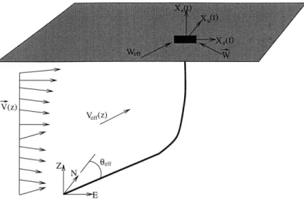
4-6 Definitions for the procedure to determine the approximate two-dimensional

plane of the mooring . . . . 75 5-1 Definitions for the hanging chains problems. . . . . 79 5-2 Power spectral density of the response of the free end of the chain for the

analytic solution and for a numerical solution with A 2 = - , At = 0.01 s,

and n = 50. ... ... . . . .. . .. . .. .. . . . . .. . .. . . 80

5-3 Power spectra peaks of the response of the free end of the chain for the analytic solution and for six variants of the generalized-a method with A t = 0.01s, and n = 50. . . . . 81

5-4 Power spectra peaks of the response of the free end of the chain for the analytic solution and for six variants of the generalized-a method with

At = 0.001s, and n = 50. . . . . 81

5-5 Power spectra peaks of the response of the free end of the chain for the analytic solution and for A' 2 - -, At = 0.001 s, with n = 50,200,400,800. 82

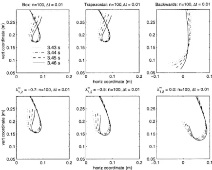
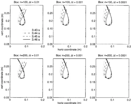
5-6 Snapshots of the chain configuration near the time of expected intersection for six variants of the generalized-a method. . . . . 83 5-7 Snapshots of the chain configuration near the time of expected intersection

for the box method with different spatial and temporal discretizations. . . . 84 5-8 Snapshots of the chain configuration near the time of expected intersection

for the trapezoidal rule with different spatial and temporal discretizations. . 85 5-9 Snapshots of the chain configuration near the time of expected intersection

for A 2 --1 with different spatial and temporal discretizations. . . . . 85

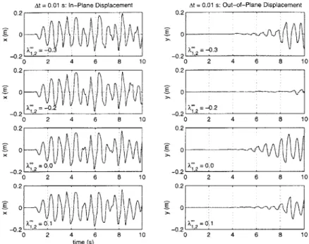
5-10 Comparison of simulation and experimental results from Howell [46], fig-ure 5.29. . . . . 86 5-11 In-plane and out-of-plane motion of the free end of the hanging chain for

the stable algorithms with At = 0.01 s. . . . . 88 5-12 In-plane and out-of-plane motion of the free end of the hanging chain for

the stable algorithms with At = 0.001 s. . . . . 89 5-13 Trace of the horizontal motions of the free end of the hanging chain for

A' = -0.3 and At = 0.001 s. . . . . 89

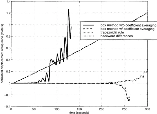
5-14 Calculated horizontal displacement of the top node of the trial mooring for the box, trapezoidal, and backward difference algorithms. . . . . 92 5-15 Shear force at the top node in the trial mooring for the three failed solution

algorithms and backward differences. . . . . 93 5-16 Calculated horizontal displacement of the top node of the trial mooring for

A',2 value of 0.0, -0.33, 0.1, and -0.2. . . . . 94

5-17 Time rate of growth of the error in the top node horizontal displacement of

the trial mooring as a function of A 2- - - -- . . .. . . 94

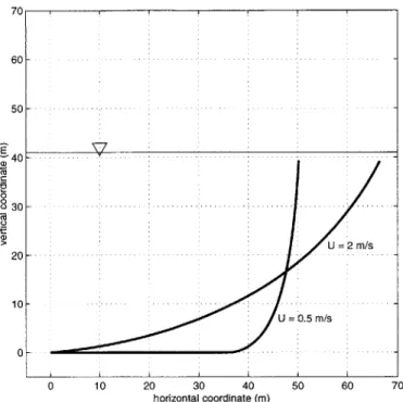
5-18 Static configuration of the trial mooring configurations in 0.5 m/s and 2.0 m /s uniform current. . . . . 95

5-20 Curvature from the static solutions of the continuous all chain mooring. . . 99

5-21 Root mean square error in the curvature of the trial solutions . . . . . 99

5-22 Mesh density after refinement of the all chain mooring. . . . 100

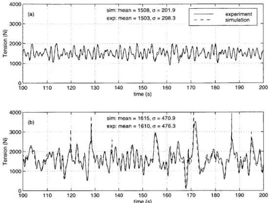
5-23 Curvature from the static solutions of the mooring with inline instruments. 101 5-24 Comparison of experimental and two-dimensional model simulated tension. 103 5-25 Comparison of experimental (a) and two-dimensional model simulated (b) acceleration signal at the lowest AxPack for the 3 January 1999 storm event. 104 5-26 Spectral comparison of experimental and two-dimensional model simulated acceleration signal at the lowest AxPack for the 3 January 1999 storm event. 105 5-27 Comparison of experimental and two-dimensional model simulated tension statistics over all 119 data sets. . . . 106

5-28 Comparison of simulated and experimental tension spectra for the 6 De-cember 1998, 0800 data record. . . . 108

5-29 Comparison of simulated and experimental tension spectra for the 3 Jan-uary 1999, 1600 data record. . . . 108

5-30 Comparison of experimental and three-dimensional model simulated tension. 109 5-31 Comparison of experimental and three-dimensional model simulated tension statistics. . . . . . .. . . . .. 110

6-1 An SDOF spring-mass-dashpot system. . . . 115

6-2 Mass values from each of the 119 spectral fits to equation 6.5. . . . 116

6-3 Damping values from each of the 119 spectral fits to equation 6.5. . . . 117

6-4 Stiffness values from each of the 119 spectral fits to equation 6.5. . . . 117

6-5 Static configurations of the simplified SWEX mooring used in the study to isolate tension mechanisms. . . . 118

6-6 (a) Mass, (b) stiffness, (c) tangential drag, and (d) normal drag coefficients calculated from simulations with isolated tension contributions. . . . 120

6-7 Fully isolated mass coefficient (circles) and mass coefficient when drag is present (x). . . . 122

6-8 Fully isolated drag coefficient (circles) and drag coefficient when mass is present (x). . . . .. . . . 122

6-9 Comparison of scatter in the relationship between

OT

Of a.. . . . 124

6-10 Comparison of scatter in the relationship between the portion of UT

at-tributable to drag and various functions of og. . . . 125 611 Total effective damping constant for the experimental spectral data, B2

-2MiKi, and the simple model total damping coefficient from equation 6.24. 128 6-12 Portion of the total tension energy attributable to each of the terms in the

variance form of the spring-mass-dashpot model, equation 6.21. . . . 130 6-13 Comparison of model predicted and experimentally observed standard

de-viation of tension. . . . 131 6-14 Comparison of model predicted tension spectra with the experimentally

observed tension spectrum for the 6 December 1998, 0800 data set. . . . 132 6-15 Comparison of model predicted tension spectra with the experimentally

observed tension spectrum for the 3 January 1999, 1600 data set. . . . 132 6-16 Variation of the model mass and drag coefficient with changes to the system

normal and tangential added mass coefficients. . . . 136 6-17 Variation of the model mass and drag coefficient with changes to the system

normal and tangential drag coefficients. _{. . . 137} 6-18 Variation of the model mass and drag coefficient with changes to the system

bottom stiffness and damping parameters. . . . 138 6-19 Model mass and drag coefficients for the simulation and experimental data

sets. ... ... 139

6-20 Total length of mooring components suspended below the surface buoy as a function of static tension. . . . 142 6-21 Comparison of experimental and model predicted a, for the CMO mooring

using a priori calculated model coefficients. . . . 146 6-22 Static configurations of the catenary riser for the simulation results. . . . . 147 6-23 Comparison of simulation and model o, for the catenary riser. . . . 149 6-24 Static configuration of the lazy wave riser for the simulation results. .-. . . 150 6-25 Comparison of simulation and model a, for the lazy wave riser. . . . 151 6-26 Simulation and model predicted values for o-, in a study using a broad range

6-27 Variation of the model mass and drag coefficient with changes to the system normal and tangential added mass and drag coefficients for both vertical and fully three-dimensional topside motion input in the simulations. . . . . 155 6-28 Model mass and drag coefficients for the three-dimensional simulation and

experim ental data sets. . . . 156 6-29 Experimental and simulated dynamic tension statistics for 126 of the data

sets from the NDBC Duck mooring. . . . 157 6-30 Simulated dynamic tension in the NDBC Duck mooring at six depths given

vertical+horizontal, vertical only, and horizontal only motion input. . . . . 159 6-31 (a) Simulated dynamic tension in the NDBC Duck mooring in 15 m depth

given horizontal only input motion. (b) Portion of dynamic tension at-tributable to drag with an initial mass estimate based on the slope of the points in (a) with TrOa, < 0.8. . . . 160

6-32 Portion of dynamic tension attributable to a stiffness effect with an initial mass estimate based on the slope of the points in figure 6-31(a) with -r-,, < 0 .8 . . . 16 2 6-33 Simulated and model fitted (equation 6.53) values for the standard deviation

of tension in response to horizontal input motion. . . . 163 6-34 Fitted stiffness coefficient for the horizontal motion model in 15, 20, 30,

and 40 m water depth. . . . 164 6-35 (a) Dynamic tension response to horizontal motion in the uniform NDBC

mooring at 15, 25, and 40 m depths. (b) Portion of the dynamic tension attributable to stiffness. . . . 165 6-36 (a) Mass coefficient fitted to the tension response data in figure 6-35(a) for

the uniform NDBC mooring at 15, 25, and 40 m depths plus additional results for 20, 30, and 35 m depths. (b) Fitted stiffness coefficient for the sam e data . . . 166 6-37 Dynamic tension response of the uniform NDBC mooring to purely

sinu-soidal horizontal input motion as a function of depth and excitation period. 167 6-38 (a) Comparison of simulated and model calculated Uh from equation 6.58.

7-1 _{The basic setup for the laboratory experiments. . . . 174} 7-2 View of the actuator shaft, load cell, test specimen, and lighting

arrange-ment looking down the flume from the anchor towards the top of the chain. 175 7-3 The foam anti-fatigue mat used as a bottom type. . . . 176 7-4 The artificial grass door mat used as a bottom type. . . . 177 7-5 View of the actuator shaft, load cell, test specimen, and bottom platform

through the glass wall of the flume. . . . 180 7-6 Example of a raw image from the video capture system. . . . 180 7-7 Edges extracted from the raw image in figure 7-6. . . . 181 7-8 Line representing the center of the model chain extracted from the edge

im age in figure 7-7. . . . 182 7-9 Tension time series for the hard bottom at Ar ~ 0.80 for excitation

ampli-tude 0.25 m and excitation periods (a) 3.0 s, (b) 2.0 s, and (c) 1.25 s. . . . 182

7-10 Tension time series for the hard bottom at Ar - 0.16 for excitation

ampli-tude 0.25 m and excitation periods (a) 3.0 s, (b) 2.0 s, and (c) 1.25 s. . . . 183 7-11 Chain response on the hard bottom over one cycle at 1.25 s excitation

period, 0.25 m excitation amplitude, and Ar ~ 0.80. . . . 184 7-12 Closeup view of the touchdown region showing a sequence in which the

chain is laid down with slack and then pulled taut. . . . 185

7-13 Definitions for the derivation of the shock criterion. . . . 186

7-14 Transverse wave and TDP speed over one cycle at 1.25 s excitation period,

0.25 m excitation amplitude, and AT ~ 0.80. . . . 189

7-15 Chain response on the hard bottom over one cycle at 2.0 s excitation period, 0.25 m excitation amplitude, and Ar ~ 0.80. . . . 190 7-16 Transverse wave and TDP speed over one cycle at 2.0 s excitation period,

0.25 m excitation amplitude, and Ar ~ 0.80. . . . 190 7-17 Chain response on the hard bottom over one cycle at 3.0 s excitation period,

0.25 m excitation amplitude, and Ar ~~ 0.80. . . . 191 7-18 Transverse wave and TDP speed over one cycle at 3.0 s excitation period,

0.25 m excitation amplitude, and AT 0.80. . . . 191

7-19 Chain response on the hard bottom over one cycle at 1.25 s excitation period, 0.25 m excitation amplitude, and Ar~ 0.16. . . . 192

7-20 Transverse wave and TDP speed over one cycle at 1.25 s excitation period,

0.25 m excitation amplitude, and Ar 0.16. . . . 193

7-21 Tension time series for the foam bottom at Ar 0.80 for excitation

ampli-tude 0.25 m and excitation periods (a) 3.0 s, (b) 2.0 s, and (c) 1.25 s. . . . 194 7-22 Tension time series for the grass bottom at /r 1 0.80 for excitation

ampli-tude 0.25 m and excitation periods (a) 3.0 s, (b) 2.0 s, and (c) 1.25 s. . . . 194 7-23 Tension time series of the initial twenty seconds for the sand bottom with

Ar - 0.16, excitation amplitude 0.25 m, and excitation periods (a) 3.0 s, (b) 2.0 s, and (c) 1.25 s. . . . 195 7-24 Changes in the sand bottom over the first 120 cycles of the 1.25 s excitation

case at A r = 0.16. . . . 196 7-25 State of the sand bottom after 120 cycles for the (a) 3.0, (b) 2.0, and

(c) 1.25 s excitation cases at Ar = 0.16. . . . 196 7-26 Tension time series for the twenty seconds preceding the 120 cycle mark on

the sand bottom at Ar a 0.16, excitation amplitude 0.25 m, and excitation periods (a) 3.0 s, (b) 2.0 s, and (c) 1.25 s. . . . 197 7-27 Simulated response with baseline parameters over one cycle at 1.25 s

exci-tation period, 0.25 m exciexci-tation amplitude, and AT 0.80. . . . 199 7-28 Simulated response with baseline parameters over one cycle at 3.0 s

excita-tion period, 0.25 m excitaexcita-tion amplitude, and Ar = 0.80. . . . 199 7-29 Simulated response with (= 0.3 over one cycle at 1.25 s excitation period,

0.25 m excitation amplitude, and Ar 0.80. . . . 200

7-30 Simulated response with ( = 0.3 and k = 1000 N/m 2 over one cycle at

1.25 s excitation period, 0.25 m excitation amplitude, and Ar = 0.80. . . .201

7-31 Simulated response with EI = 0.01 N/m 2 over one cycle at 1.25 s excitation

period, 0.25 m excitation amplitude, and Ar = 0.80. . . . 202 7-32 (a) Tension at the top of the mooring and (b) TDP speed and transverse

wave speed at the TDP for a portion of a simulation of the full scale SWEX mooring using environmental conditions from the 3 January 1999 storm event. 204 7-33 Maximum difference in the wave and TDP speeds during unloading for

7-34 Maximum difference in the wave and TDP speeds during loading for simu-lations with sinusoidal excitation. . . . 206 A-i Vector definitions for the local coordinate system. . . . 216 A-2 Schematic diagram of pressure and effective tension terms. . . . 218 C-1 Error and relaxation factor during the static solution of a mooring problem

with line on the bottom . . . 236

F-1 m and Cd coefficients calculated in 500 distinct bootstrap Monte Carlo

sim ulations. . . . 250 F-2 Probability density function for m based on 20000 distinct bootstrap Monte

Carlo sim ulations. . . . 252

F-3 Probability density function for Cd based on 20000 distinct bootstrap Monte

List of Tables

2.1 Algorithms included in the generalized-a method. . . . . 46

4.1 Properties of the components used in the experimental mooring. . . . . 68

5.1 Comparison of the predicted cross-over time and total simulation time be-fore failure for three-dimensional simulations of the forced hanging chain . 87 5.2 ak, am, and -y values for the tested algorithms. . . . . 91 5.3 Mass and drag coefficients for the validation simulations. . . . 102 5.4 Tension statistics for the comparison data sets. . . . 110 6.1 Variations on the mooring properties used in the simulations to isolate

individual tension mechanisms. . . . .. 119 6.2 Parameter variations considered in the model coefficient functional

depen-dence study...135

6.3 Non-dimensional mean tension and <p values for the catenary riser and lazy wave riser system s. . . . 148 6.4 Error in the model predicted og for the catenary riser using a priori model

coefficients. . . . 148 6.5 Fitted coefficients for the dynamic tension response to horizontal motions

using the same model form as for vertical motions. . . . 161 6.6 Fitted coefficients with 95% confidence intervals for the dynamic tension

response to horizontal motions using the model described by equation 6.53. 162 7.1 Friction coefficients, in air, of the various bottom types. . . . 177 7.2 Number of correct and incorrect predictions given a probability level of 0.9

Chapter 1

Introduction

A mooring system is typically understood as any type of cable, chain, rope, or tether assembly that connects a floating or subsurface buoyant object (ship, buoy, platform) to an anchoring system fixed on the sea floor. The floating object will move with environmental forcing, but the mooring system will contain the movements to some area (the watch circle) centered about the anchoring system. Any mooring system must provide compliance or flexibility to accommodate deformations induced by currents and by forcing with periods ranging from hours (tides) to seconds (wind waves) without over-tensioning the system

components.

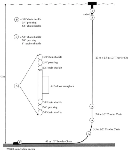
This flexibility is typically achieved either through the use of elastically compliant members such as rubber tethers or long lengths of synthetic rope, or through geometrically compliant configurations in which the system accommodates deformations by changing shape without stretching. The geometrically compliant approach is more common in situations where adequate compliance or a combination of strength and compliance cannot be provided by taught elastic members. This is the case in extremely shallow water, where the lengths of the rope or tethers are so short as to limit their compliance. Geometric compliance is also often found in offshore deep water applications where the pipe sections can be made relatively flexible in bending (through the use of short lengths of pipe and flexible joints), but not in axial stretching. Examples of geometrically compliant mooring shapes are shown in figure 1-1.

The shallow water mooring shown in figure 1-1(a) illustrates the type of mooring typi-cally used to moor oceanographic, meteorological, and aids-to-navigation buoys in shallow

Figure 1-1: Examples of geometric compliance in mooring and riser systems: (a) shal-low water buoy mooring, (b) deep water oceanographic mooring, and (c) lazy wave riser configuration.

water (on the order of 100 m) [5, 13]. The typical mooring for this sort of application consists entirely of lengths of chain, with instruments possibly attached between chain segments. We say that this type of system is geometrically compliant because its primary mechanism to accommodate the motion of the buoy is to lift and lower chain to and from the bottom, thus changing its shape. As long as chain remains on the bottom in the steady state configuration, the system is typically more flexible geometrically than it is elastically.

The advantages to this arrangement include very high strength due to the use of chain as the primary strength member, and the ability to deploy this configuration in a variety of water depths. The primary disadvantage to this type of mooring is the need for regular replacement of the chain near the bottom of the mooring due to the abrasion of the chain on the sea bed [5,23]. A recent alternative to this type of mooring uses elastic tethers as the primary compliance mechanism [57,77]. These systems feature significantly reduced tensions in most sea conditions because of the much lower mass of the tethers compared to chain moorings. Drawbacks to elastic tether moorings include the inability to place instruments along the tether and their susceptibility to cutting, either in an accident or through vandalism.

The second type of system in figure 1-1 is an increasingly popular configuration for deep water surface moorings for oceanographic applications [31]. Variations on this shape are also used to moor meteorological buoys [13]. The s-curve in the mooring shape is achieved through careful placement of flotation and ballast along the line. The location of this curve at mid-depth allows for geometric compliance without a rigid bottom. Previous deep water

surface moorings achieved compliance through the incorporation of long lengths of highly stretchable synthetic rope [5]. The advantage to the geometrically compliant system in figure 1-1(b) is the ability to run conductive electromechanical cable along the full length of the mooring to bring signals from subsurface instruments to the surface for telemetry. Elastically compliant electromechanical members have only recently been introduced [75, 76] in the oceanographic community and are difficult to handle and relatively expensive, particularly for very long lengths.

Both of the above described mechanisms, an s-shape at mid-depth, and a catenary shape along the bottom are often employed together in offshore energy production systems, as pictured in figure 1-1(c). In this case the mooring line of interest is typically a pipe running from the platform to the wellhead. The platform may also be anchored (anchoring lines not shown in figure 1-1(c)) at multiple points by taut synthetic lines or heavy chain and wire lines forming a catenary similar to that described for the shallow water buoy mooring. The need for geometric compliance in the riser pipe arises from the inflexibility of these pipes to axial (elastic) deformation.

As a final consideration in this brief overview of compliant moorings, it should be noted that in addition to achieving compliance through the mooring line, either geometrically or elastically, it is possible in some cases to introduce compliance at the surface by using buoys or platforms which have a very low natural frequency (very far below typical wave frequencies) such as a spar buoy. This effectively puts a very soft compliant element between the wave forcing and the mooring line. Because spar buoys are very long and slender, they typically have low reserve buoyancy and are difficult to handle.

All of the systems pictured in figure 1-1 provide significant compliance to surface wave motions under most conditions. One well known mode under which these configurations do not provide good compliance is in the case of large currents that pull the geometric shaping out of the mooring. The impact of this failure mode can be lessened with the addition of elastic compliance into the design. The geometric compliance in these systems can also break down during a large storm in which the ability of the mooring to change shape may be limited by fluid drag on the cable. This second failure mode is more difficult to design for as it can occur even in conditions under which the static shape is preserved and may not be alleviated by secondary elastic compliance. Finally, for cases with cable resting on the sea floor, friction, adhesion and the elasticity of the bottom can affect the

ability of the system to deform geometrically. A loss of geometric compliance as a result of any of these mechanisms can lead to dangerously high tensions. A detailed analysis of geometrically compliant systems, which will lead to better prediction of these types of failures, is the primary goal of this thesis.

1.1

Analysis of compliant systems

Much of the recent analytical work relating to geometrically compliant systems has been conducted in the context of calculating the contribution of the mooring line damping to the overall system dynamics. Brown et al. [7] provide a review of much of the literature to date in this area. Most of the work has focused on frequency domain quasi-linearized numerical solutions for the slow drift case. Extensive model scale tests have also been

carried out [55, 59, 67].

Large floating structures (ships, offshore platforms) typically have little damping and low natural frequencies for motions in the horizontal plane. For these large structures, mooring tensions at wave frequencies are much smaller than the excitation forces. At lower frequencies, the mooring forces and wave forces are more comparable. Thus, the damping provided by the motion of the mooring system plays a critical role in the response of these structures to slow drift motions [59, 96].

Motions and dynamic tension at wave frequencies are often ignored in these studies. This allows for a simplified treatment of the dynamics. For example, Nakamura et al. [67] used catenary formulae to calculate the integrated quasi-static velocity and acceleration along the mooring. These integrated motions allowed them to write the dynamic tension due to slow drift motions in a very simple form.

In the analyses of compliant systems developed in this thesis, the quantity of interest is typically dynamic tension rather than platform motion. Such an approach is particularly relevant in oceanographic applications where the motion of the surface platform may not be critical, but dynamic tension is dominated by wave induced motions. Knowledge of the tension is critical in these applications because components are typically not specified with large safety factors for fatigue and ultimate failure (both for cost and ease of handling reasons).

drift damping problem. Huse and Matsumoto [52-55] used a linearized finite element model to compute the mooring line damping in the presence of a slow drift regular motion superposed with a spectrum of high frequency first-order wave motions. Their calculations showed that the damping was two to four times higher when the high frequency motions were taken into account. Similar results were obtained by Dercksen et al. [22] and Fylling et

al. [32] with more sophisticated numerical models.

In other work that looked at both slow drift and wave frequency excitation, Web-ster [99] characterized the mooring line damping of a non-dimensionalized catenary riser system (a system shaped like that shown in figure 1-1(a)) as a function of static tension, excitation frequency and amplitude, scope, stiffness, drag, and current. The excitation was sinusoidal and either purely vertical or purely horizontal. The numerical model that he used was a time-domain nonlinear finite element code.

Webster [99] also briefly touches on the "impedance" of mooring systems which he describes in terms of the trade-offs between geometric and elastic compliance. This is a concept first introduced by Triantafyllou et al. [94] to characterize the ratio of elastic to catenary stiffness. They noted that fluid drag limits the ability of the mooring to deform geometrically and as a result, dynamic tensions increase.

1.2

Bottom interaction

An important part of the response in many geometrically compliant systems is the inter-action of grounded line with the sea floor. Several recent papers have described numerical methods for modeling this interaction [16,56,63,89, 90]. To date, however, these models have not been used to extensively analyze the implications of the bottom interaction on the total mooring response.

Thomas and Hearn [91] and Liu and Bergdahl [63] examined the bottom interaction problem in the context of mooring line damping. The results from both papers suggest that bottom interaction effects do contribute to mooring line damping, with the in-plane friction being more important than the out-of-plane effects [91].

Aranha et al. [2], Pesce, Aranha, and Martins [79], and Pesce et al. [80] have examined the curvature of riser pipes in the touchdown region using an analytical boundary layer approximation. Their goal is to provide better predictions of the bending moment to

re-duce fatigue failures. Some of the background for their analytical approach comes from work by Burridge et al. [12] and Burridge and Keller [11] for the motion of a string on a unilateral constraint. That work demonstrated that a shock wave will form when the velocity of the touchdown point exceeds the transverse wave speed of the cable. The ana-lytical development in Aranha et al. [2] assumes that the touchdown point speed is always below this critical limit. No work has been performed that examines the implications for mooring dynamics when this assumption does not hold and shock waves do form.

1.3

Modeling tools

The problem of predicting the steady state configurations and transient motions of pipe, hose, cable, chain, and rope systems in a marine environment is encountered in numerous applications. Oftentimes, the methods of solving the problem seem equally numerous. Buoy and ship moorings, offshore platforms, and towed systems are often analyzed in very different ways, yet are at heart very similar types of structural systems.

In a 1970 survey paper, Casarella and Parsons [14] compiled an extensive list of work related to the hydrodynamic response of cable systems. Their history starts with analytical work dating from 1917 to calculate the steady state configuration of cables in air. Through 1950, treatments of the steady state problem dominated the literature in this area, with the first dynamic models for cables in water appearing in 1957. Thomas [90] provides a detailed summary of the development of the modern dynamic models, beginning with Walton and Polachek's paper in 1960 [98], and emphasizing developments in the literature from the offshore energy field.

The model developed as part of this thesis provides a nonlinear time-domain solution to the mooring dynamics problem. The other modern models described below can be similarly classified. Other types of models include frequency domain and linearized or quasi-static time domain models. While attractive for their computational efficiency, these latter types of models are typically not used for the types of highly nonlinear motions that are inherent in the phenomena that are analyzed in the thesis.

1.4

State-of-the-art time-domain models for mooring

sys-tems

Numerical models for mooring systems can be categorized in several different ways. The most often cited distinguishing characteristic of a model is the method used to discretize the physical system in space. Among the most common methods are finite elements, finite differences, and lumped parameter. While there is more universal agreement on the temporal discretization method (most use finite differences), there is some variation in the way that the temporally discretized equations are integrated in time. Beyond these distinctions are the mathematical and physical features incorporated by the various models such as bending stiffness, sea bed interaction effects, and treatment of vortex-induced vibrations.

1.4.1 Spatial discretization

Walton and Polachek [98] published the first treatment of the dynamic solution that re-sembles very closely the solution methods in use today. They formulate the equations of motion for discrete elements and use centered finite differences to discretize the time deriva-tive terms and step the solution forward in time. With the addition of cable extensibility by Polachek et al. [81], a remarkably complete treatment of the nonlinear time domain problem existed as early as 1963. This first solution, using a force balance on discrete elements to write the equations of motion is what we now categorize as a lumped parame-ter method. The parame-terminology arises from the lumping of the mass and exparame-ternally applied forces at adjacent nodes which are joined by massless springs. This discretization approach has an intuitive simplicity to it and as such is relatively easy to implement. Recent models that make use of this approach are described by Huang [47] and Thomas [90,91].

In contrast to the summation of forces approach used by lumped parameter methods, finite element methods derive their governing equations through principles of virtual work. One advantage of this approach is the possibility of a more sophisticated treatment of mass. Lumped parameter derivations must necessarily place all mass at discrete nodes and then write the governing equations. Finite element methods can derive the governing equations using an integration of the mass over the entire element, thus leading to the "consistent" mass formulation [62]. The starting point for finite element methods as

applied to the marine cable problem is typically a discrete element, much like the lumped parameter methods. Examples of such derivations include Engseth [28] and McNamara et al. [64]. Paulling and Webster [78], following Garrett [33], take the alternative approach of formulating differential equations of motion which are solved by the substitution of a discrete collection of shape functions which minimize the element energy. The majority of state-of-the-art programs currently being used for riser modeling are based on finite elements [611.

A third approach is to write the continuous partial differential equations and then ap-ply a spatial discretization scheme based on finite differences. This is the approach taken by Ablow and Schechter [1] among others. We distinguish between this and lumped pa-rameter methods based on the starting point, which in this case is an infinitesimally small differential element and in the lumped parameter case is a finite discrete element. Given similar physical assumptions the two methods are entirely equivalent, as demonstrated by Huang [47]. The distinction between this and the lumped parameter approach is based largely on the applications of the method. Many of the numerical solutions for tow cable dynamics have used finite differences of the continuous partial differential governing equa-tions. Another reason for the distinction in this case is simply that, to date, most pure lumped parameter methods do not include the effects of bending stiffness in the equations of motion [91]1. Authors deriving continuous forms of the governing equations have easily incorporated this effect [10,46,93]. The model development detailed in chapter 2 is based on this approach.

Finally, a few alternatives to the spatial discretizations outlined above have appeared in the literature. Chiou and Leonard [17] and Sun et al. [86] describe the Direct Inte-gration Method, whereby a boundary value problem is recast as a set of initial value problems. Each initial value problem is integrated spatially from a boundary with known boundary conditions, and the solutions from these integrations are combined to form a total solution that satisfies all boundary conditions. Because the initial value approach allows for explicit numerical integration in space, the method has the advantage that the solution of large linear systems of equations typical in implicit finite difference and finite element schemes can be avoided. There is of course a spatial discretization implied by the

Buckham and Nahon [9] have recently incorporated bending effects into a lumped parameter model for low tension ROV tethers.

numerical integration of the transformed governing equations. Sun et al. [86] point out the need for a method to suppress any spurious solution components that may grow as the spatial integrations proceed along the cable. Another alternative scheme is collocation which breaks the cable into a small number of segments and fits high order Chebyshev

polynomials as a solution to the governing equations over each region [15].

1.4.2 Temporal discretization

For all spatial discretization methods the resulting equations are typically written as a non-linear matrix equation known as the semi-discrete equation of motion, because the time derivatives of the vector of dependent variables are left as continuous functions. The exception to this procedure is in finite difference based solutions which typically are differenced both in space and in time as part of the same process. This leads to yet another distinction between lumped parameter and finite difference approaches. The starting point for a finite difference method is typically a set of first-order hyperbolic partial differential equations. The equations of motion for lumped parameter schemes are most often presented in matrix form as a system of second-order ordinary differential equations - the semi-discrete equation of motion.

Most temporal integration schemes in use today have their roots in the method devel-oped by Newmark [70]. Hughes and Belytschko [50] provide a summary of the development of these types of methods in the context of linear finite element structural dynamics. The methods typically employ temporal finite differences, with a variety of different schemes used to interpolate the solution over the time step. Most classical methods can now be cast into unified multi-parameter integration schemes where an adjustment in the parameters leads to one of several different methods with different numerical properties (e.g., [44,100,102]). Thomas [90] studied the three "classic" methods (Newmark, Houbolt, and Wilson-0) and their applicability to the mooring dynamics problem. He concluded that Houbolt was the best choice. This is not a surprising result - earlier, Park [74] noted that Houbolt was a good choice for highly nonlinear problems. Thomas did not consider any of the more modern developments in time integration that are taken up in more detail

in chapter 2.

In addition to Newmark and its variants which are popularly employed with finite element based models, researchers in the cable dynamics field have employed a variety of

different schemes for the temporal integration problem. Chiou and Leonard [17] use simple backward finite differences. Sun et al. [86] use the generalized trapezoidal rule which is a first-order variant of the Newmark method; it will be discussed in some detail in chapter 2.

Garrett [33] and Paulling and Webster [78] use the Adams-Moulton method, which in

first-order form reduces to the trapezoidal rule. Sanders [84] used a computationally expensive but fourth-order accurate Runge-Kutta procedure. This is unusual in that most researchers have accepted first- or second-order accuracy in order to reduce computational expense.

The most popular finite difference scheme is the box method, in which the governing equations are discretized on the half-grid point in both space and time. This method was first employed for the solution of tow cable dynamics by Ablow and Schechter [1]. Since then it has been employed in both towing and mooring applications by Milinazzo et al. [65], Howell [46], Tjavaras [93], and Chatjigeorgiou and Mavrakos [15] among others. As will be shown, the temporal portion of this discretization is a special form of the generalized-a method to be developed in chapter 2. That development will also demonstrate that the box method is seldom the best choice of temporal discretization schemes for the cable dynamics problem. In a recent paper, Koh et al. [60] came to this same conclusion and proposed a modified box method that used backward differences for the temporal discretization.

1.4.3 Forcing, boundary, and material effects

There is little disagreement in the proper method of incorporating fluid forces, including buoyancy, viscous drag, and added mass forces, into state-of-the-art numerical codes. As late as 1970, Casarella and Parsons [14] did choose to distinguish between models according to the treatment of drag and whether or not tangential drag was included, but there do not appear to be any significant differences between modern approaches. Likewise, Breslin [6] laid the groundwork for a consistent treatment of buoyancy and effective tension in modern codes. One significant source of hydrodynamic forcing that has not yet been fully incorporated into a nonlinear time domain code is vortex-induced vibrations. This is an area of active research [95].

The numerical treatment of the interaction of the cable with the sea bed is also an area of active research. Three basic approaches are prevalent in the literature. Frequency domain models (e.g., [94]) and some time domain models (e.g., [89]) cut the mooring off

at the touchdown point and attach an equivalent linear spring and/or dashpot. This approach is only valid for small dynamic motions about the static touchdown point. A second method is the lift-off and grounding approach described by Nakajima et al. [66] and Thomas [90]. In this method, the mass of the discrete nodes or elements is reduced to zero as they approach the bottom. This simulates a perfectly rigid bottom with no impact loads (a smooth rolling and unrolling of the cable, similar to the analytical calculations of Aranha et al. [2]). Thomas noted significant numerical difficulties associated with the implementation of lift-off and grounding. The third approach is to model the sea bed as an elastic foundation. This method has been used by Inoue and Surendran [56] and Webster [99]. It is relatively easy to implement and places few restrictions on the types of systems that can be modeled. The primary difficulty with this method is in determining appropriate elastic and damping constants to associate with a given type of soil. The elastic foundation approach is the basis for the bottom interaction model developed as part of this thesis.

For material effects, modern codes may or may not include the effects of material non-linearities or bending stiffness. There is little disagreement, however, on the conditions under which these effects should be included if an accurate response calculation is to be made. Most finite element codes, developed for riser systems that are built from relatively large diameter metal pipes, do include bending stiffness, but may neglect material non-linearities without a significant loss of accuracy. In the oceanographic community where small diameter synthetic mooring lines are common, material nonlinearities can be impor-tant and bending stiffness can often be neglected. Some codes employ a hybrid approach whereby bending stiffness is included only in low tension regions as a numerical smooth-ing effect (e.g., [87]). A general purpose code should allow for both linear and nonlinear materials and for materials with and without bending stiffness.

1.5

Overview of the thesis

Chapter 2 describes the development of the generalized-a method for the time integration of the cable equations. As an example, the governing continuous partial differential equa-tions for mooring lines in two dimensions are presented and the reduction to semi-discrete form, using spatial finite differences, is derived. The analysis of the stability of a time

integration scheme is introduced using the stability of the box method as an example. Potential problems with the box method are described and alternative methods are ex-plored. The generalized-a method is introduced and the stability and accuracy of the method as applied to the cable equations are presented. Comparison is made between the new method and many of the previously used methods, including backward differences and the generalized trapezoidal family.

Additional details about the numerical program, including boundary conditions and the handling of bottom interaction effects, are described in chapter 3. The algorithms used for spatial mesh refinement and adaptive time stepping are also described. Details not provided in chapter 3 are given in the appendices.

The field experiment is described in chapter 4. The centerpiece of the experiment was a heavily instrumented all chain mooring. Mooring hardware and instrumentation are described. Calibration and data quality issues are also discussed.

The model is validated and the numerical parameters used in the model are studied in chapter 5. The validation is based on analytical and experimental results for a laboratory scale hanging chain problem and on full-scale mooring data from the experiments described in chapter 4.

Chapter 6 details a statistical and analytical study of the different contributions to the dynamic tension in geometrically compliant systems. These contributions are char-acterized as drag, stiffness (geometric and elastic), and inertia. The study is based on experimental data and extensive numerical runs. Statistical and spectral analyses are used along with parametric numerical studies to isolate each of the different tension mech-anisms. The result of these analyses is a very simple model that can be used to predict dynamic tension given a basic characterization of mooring properties, steady state tension, and sea state parameters. The chapter concludes with an investigation of the effect of the directionality (vertical, horizontal, vertical and horizontal, fully three-dimensional) of the input motion.

A detailed examination of the interaction between the mooring line and the bottom is presented in chapter 7. This includes numerical and laboratory simulations of cases where there is significant buckling of the line in the region near the touchdown point. The implications of the shock condition at the touchdown point are also considered.

1.6

Original contributions

The numerical program developed in this thesis is based on that of Tjavaras [93] and Howell [46]. In the thesis, the program is extended to include bottom interaction effects and adaptive discretizations in time step and mesh density. A new temporal integration scheme, the generalized-a method, is developed and placed in the context of the recent structural analysis literature. An analysis of the stability and accuracy of the overall procedure is presented and comparisons are made with other schemes. The new procedure has substantially improved stability properties when compared to the old method. The model validation detailed in chapter 5 is new for this particular numerical model.

The analysis of dynamic tension in geometrically compliant systems in chapter 6, using regular and random, vertical, horizontal and three-dimensional input motions, and a broad range of hydrodynamic and material parameters, is more extensive than any of the previous work in this area. The approach to and the development of the simple formula for predicting dynamic tension in these system is unique to this thesis.

Finally, the consideration of the extreme responses of the mooring line on the bottom is new. Previous authors [2,94] have limited their analyses to the subsonic case. This is the first time that the shock criterion has been experimentally verified and the implications of the tension shocks observed and discussed.

Chapter 2

Development of the Time

Integration Algorithm

2.1

Governing partial differential equation

Detailed derivations of the three-dimensional dynamic governing equations for a cable with bending stiffness suspended in water are provided by Tjavaras [93]. For completeness, a derivation of the two-dimensional equations, upon which the analyses presented in this chapter are based, is provided in Appendix A. While the procedure developed below can be applied equally well to both two- and three-dimensional models (as will be illustrated through the use of both in subsequent chapters), the two-dimensional equations are used here for simplicity and succinctness; the two-dimensional model requires six equations where the three-dimensional model requires thirteen. The two-dimensional equations for