Comparison of emissions from on-road sources using a mobile laboratory under various driving and operational sampling modes

(1)

Comparison of emissions from on-road sources using a mobile

laboratory under various driving and operational sampling modes

The MIT Faculty has made this article openly available.

Please share

how this access benefits you. Your story matters.

Citation

Zavala, M. et al. “Comparison of Emissions from On-road Sources

Using a Mobile Laboratory Under Various Driving and Operational

Sampling Modes.” Atmospheric Chemistry and Physics 9.1 (2009) :

1-14. © Author(s) 2009

As Published

http://dx.doi.org/10.5194/acp-9-1-2009

Publisher

European Geosciences Union / Copernicus

Version

Final published version

Citable link

http://hdl.handle.net/1721.1/65133

Terms of Use

Creative Commons Attribution 3.0

(2)

www.atmos-chem-phys.net/9/1/2009/

Chemistry

and Physics

Comparison of emissions from on-road sources using a mobile

laboratory under various driving and operational sampling modes

M. Zavala1,2, S. C. Herndon3, E. C. Wood3, J. T. Jayne3, D. D. Nelson3, A. M. Trimborn3, E. Dunlea2,*,

W. B. Knighton4, A. Mendoza5, D. T. Allen6, C. E. Kolb3, M. J. Molina2,7, and L. T. Molina1,2

1_{Molina Center for Energy and the Environment, San Diego, California, USA}

2_{Department of Earth, Atmospheric and Planetary Sciences, Massachusetts Institute of Technology, Cambridge,} Massachusetts, USA

3_{Center for Atmospheric and Environmental Chemistry, Center for Cloud and Aerosol Chemistry, Aerodyne Research Inc.,} Billerica, Massachusetts, USA

4_{Department of Chemistry, Montana State University, Bozeman, Montana, USA} 5_{Departamento de Ingenier´ıa Qu´ımica, Tecnol´ogico de Monterrey, Monterrey, M´exico} 6_{Center for Energy and Environmental Resources, University of Texas, Austin, Texas, USA} 7_{Department of Chemistry and Biochemistry, University of California, San Diego, California, USA}

*_{now at: National Oceanic and Atmospheric Administration, Climate Program Office, Silver Spring, Maryland, USA} Received: 26 March 2008 – Published in Atmos. Chem. Phys. Discuss.: 23 April 2008

Revised: 15 October 2008 – Accepted: 17 November 2008 – Published: 6 January 2009

Abstract. Mobile sources produce a significant fraction of

the total anthropogenic emissions burden in large cities and have harmful effects on air quality at multiple spatial scales. Mobile emissions are intrinsically difficult to estimate due to the large number of parameters affecting the emissions vari-ability within and across vehicles types. The MCMA-2003 Campaign in Mexico City has showed the utility of using a mobile laboratory to sample and characterize specific classes of motor vehicles to better quantify their emissions charac-teristics as a function of their driving cycles. The technique clearly identifies “high emitter” vehicles via individual ex-haust plumes, and also provides fleet average emission rates. We have applied this technique to Mexicali during the Bor-der Ozone Reduction and Air Quality Improvement Program (BORAQIP) for the Mexicali-Imperial Valley in 2005. We analyze the variability of measured emission ratios for emit-ted NOx, CO, specific VOCs, NH3, and some primary fine particle components and properties by deploying a mobile laboratory in roadside stationary sampling, chase and fleet average operational sampling modes. The measurements re-flect various driving modes characteristic of the urban fleets. The observed variability for all measured gases and particle emission ratios is greater for the chase and roadside station-ary sampling than for fleet average measurements. The fleet

Correspondence to: M. Zavala

(miguelz@mce2.org)

average sampling mode captured the effects of traffic con-ditions on the measured on-road emission ratios, allowing the use of fuel-based emission ratios to assess the validity of traditional “bottom-up” emissions inventories. Using the measured on-road emission ratios, we estimate CO and NOx mobile emissions of 175±62 and 10.4±1.3 metric tons/day, respectively, for the gasoline vehicle fleet in Mexicali. Com-parisons with similar on-road emissions data from Mexico City indicated that fleet average NO emission ratios were around 20% higher in Mexicali than in Mexico City whereas HCHO and NH3emission ratios were higher by a factor of 2 in Mexico City than in Mexicali. Acetaldehyde emission ratios did not differ significantly whereas selected aromatics VOCs emissions were similar or smaller in Mexicali. Ni-trogen oxides emissions for on-road heavy-duty diesel truck (HDDT) were measured near Austin, Texas, as well as in both Mexican cities, with NOy emission ratios in Austin < Mexico City < Mexicali.

1 Introduction

Emissions from transportation sources, primarily on-road motor vehicles, are generally the largest contributors to cri-teria air pollutants such as CO, NOx, and selected volatile organic compounds (VOCs) in urban areas; on-road vehicles are also major sources of fine primary particle emissions and

(3)

2 M. Zavala et al.: Variability of mobile emissions sampled using a mobile laboratory

specific air toxics (Molina et al., 2004). Despite their im-portance in determining air quality levels, the estimation of mobile emission sources is challenging because multiple pa-rameters affect the variability of on-road mobile emissions within and across vehicles types (Cadle et al., 2007). Factors such as engine size and type, fuel composition, temperature and pressure are directly linked to the combustion efficiency (and therefore the emission rates) of in-use vehicles; other external factors such as driving conditions and the character and maintenance of fuel delivery and emission control sys-tems also decisively affect the variability and composition of mobile emissions (NARSTO, 2005).

Laboratory studies have shown a strong dependency of pollutant emissions on vehicle velocity and engine load (e.g. Ntziachristos and Samaras, 2000; Joumard et al., 2000; An-dre et al., 2006). However, vehicle speed and acceleration under real-world operating conditions are affected by traf-fic congestion, road infrastructure (e.g. traftraf-fic signals and posted speed limits) and even personal driving behaviors. The combination of these operating conditions impacts the engine load and therefore the pollutant emissions rates. On-road emission measurements have also shown a strong de-pendence of pollutant emissions on vehicle speed and engine load (Pierson et al., 1996; Kean et al., 2003; Chan et al., 2004). The variability of emissions on vehicle speed and en-gine load has been found to be higher when emissions are ex-pressed by distance travelled as compared to fuel consumed. A similar dependency of the effects of driving conditions (categorized for example by idling, acceleration and cruis-ing modes) on vehicle emissions has been found in a more limited number of on-road measurement studies (Tong et al., 2000; Shah et al., 2006; Durbin et al., 2008).

Because the vehicle fleet in an urban area is composed of a large number of vehicle types, “fleet-average” emission characteristics have an associated intrinsic variability. In this work, “fleet-average” describes conditions where individual exhaust plume emissions from a large number of vehicles are captured during sampling; the longer the sample data ex-tends, the more probable the overall emission characteristics of the fleet are captured. The observed variability during the measurement of on-road emissions in fleet average driving conditions is the result of the individual emission variability from a wide range of sampled vehicles. As a result, point estimates (e.g. average emissions of a given pollutant) of the rate of mobile emissions in an urban area are of limited value unless a description of their associated variability is avail-able.

Cross-validation and inter-comparisons of mobile emis-sion measurements using different emisemis-sion measurement techniques are important and useful. Solid data can be ob-tained from inter-comparisons using different emission mea-surement techniques such as remote sensing, mobile labo-ratories, dynamometer and tunnel studies (e.g. Sj¨odin and Lennerb, 1995; Walsh et al., 1996; Kean et al., 2003). How-ever, appropriate consideration of the different conditions

un-der which the measurements were made is very important for the inter-comparisons due to the differences in sampling times and frequencies, pollutant measurements instrumenta-tion, sample size and analysis assumptions for each measure-ment.

During the MCMA-2003 Field Campaign, the Aerodyne Research Inc. (ARI) mobile laboratory was deployed in the Mexico City Metropolitan Area (MCMA) to sample and characterize specific classes of motor vehicles to better quan-tify their emissions characteristics as a function of their driv-ing cycles (Molina et al., 2007). Emission ratios (defined as the above background pollutant concentration normalized to excess CO2concentration) for NOx, NOy, NH3, H2CO, CH3CHO, and other selected VOCs were estimated for chase sampled vehicles in the form of frequency distributions and for the fleet averaged emissions (Zavala et al., 2006). The results indicate that the technique is capable of differentiat-ing among vehicle categories and fuel type under real world driving conditions. We extended this technique to Mexicali, Baja California, Mexico during the BORAQIP program for the Mexicali-Imperial Valley in 2005 (Mendoza et al., 2007). This paper discusses the measurements of on-road mo-bile emissions obtained from 12–23 April 2005 in Mexicali during the field campaign under different driving and op-erational sampling modes using the ARI mobile laboratory. The driving modes represented various speed and congestion characteristics of the sampled fleet. We present a compari-son of the on-road emission measurements in Mexicali with corresponding measurements obtained during the MCMA-2003 field campaign (Molina et al., 2007). This constitutes a unique opportunity to compare the vehicle fleet emission characteristics of a megacity and a smaller urban area in the same developing country. Since the measurements were ob-tained using the same technique, assumptions and instrumen-tation in the two campaigns, the observed differences in the comparison are more likely to be the result of actual differ-ences in fleet emission characteristics between the two cities. In addition, during 8–9 May 2003 the ARI mobile laboratory obtained on-road measurements of heavy-duty diesel trucks (HDDTs) in and near Austin, TX in order to capture Mex-ican and US HDDTs emissions using the chase technique. We also compare the results obtained in Austin, with mea-surements obtained from individual HDDTs in Mexico City and Mexicali.

2 Methodology

The mobile laboratory deployed during the Mexicali field campaign was equipped with several high time resolution and high sensitivity instruments as described in detail in Kolb et al. (2004), Herndon et al. (2005), and Zavala et al. (2006). These included Tunable Infrared Laser Differential Absorp-tion Spectroscopy (TILDAS) instruments for measuring se-lected gaseous pollutants, a Proton Transfer Reaction Mass

(4)

Spectrometer (PTR-MS) for measuring selected VOCs, a commercial NO/NOychemiluminescent detector operated in 1-s mode, and a Licor Non-Dispersive Infrared (NDIR) in-strument for CO2. An Aerosol Mass Spectrometer (AMS), a Condensation Particle Counter (CPC) and a Multi Angle Absorption Photometer (MAAP) were also deployed to re-trieve information regarding the composition, number and light absorbing (black carbon) characteristics of emitted par-ticles. High sensitivity and high time resolution (1–2 s) in-strumentation allows the mobile laboratory to capture the temporal pollutant concentrations variability of the turbulent exhaust plumes as they are dispersed into the surrounding air. Other instruments on board the mobile laboratory included a Global Positioning System (GPS), an anemometer and a video camera used to obtain target vehicle information. The mobile laboratory’s velocity and acceleration were measured and recorded continuously to characterize the driving mode conditions during the sampling. Local atmospheric param-eters including pressure, temperature, and relative humidity were also measured continuously.

For the Mexicali study, most measurements were made while driving on city streets. There were no precipitation events during the sampling periods. A total of 98 valid mo-bile emission ratio experimental periods were obtained dur-ing the analysis of 14.5 h of on-road and roadside data. The samples comprised a variety of driving modes (e.g., idling, acceleration, cruising, etc.), fuel types (gasoline and diesel), vehicle model years, and vehicle types (light-duty gasoline vehicles (LDGVs) and HDDTs). Three types of operational sampling modes were used to obtain on-road vehicle emis-sion data: 1) individual identified vehicle emisemis-sion plumes measured by roadside stationary sampling; in this mode, emission ratios from individual emission plumes were ob-tained during periods of stationary sampling along the road whenever the wind was favourable for transporting the ve-hicle’s emissions to the mobile laboratory sampling port; 2) chase experiments where the mobile laboratory followed spe-cific vehicles, primarily heavy-duty diesel trucks and buses, repeatedly sampling their exhaust plumes for several min-utes; and 3) on-road fleet average sampling modes where no attempt was made to distinguish plumes from individual ve-hicles and all intercepted vehicle emissions plumes from both passing and incoming vehicles are counted and weighted equally; in this mode, emission ratios were obtained by ana-lyzing the periods in which the emission signatures from sur-rounding vehicles were sufficiently mixed by the time they were sampled by the mobile lab.

The specific analytical procedures for obtaining the emis-sion ratios in the aforementioned operational sampling modes have been described by Herndon et al. (2004) and Zavala et al. (2006). Briefly, the analysis of the multiple, synchronized, instruments on board the mobile laboratory allows the identification of targeted emission plumes. Other discriminators used to distinguish against possible sources of pollutants other than nearby mobile sources are: 1) readings

from the anemometer to identify the direction and speed of the incoming wind at the sampling port, which identifies pe-riods of possible “self sampling” of the mobile lab exhaust; 2) images obtained with the video camera for observing and classifying nearby vehicles; and, 3) real-time data log notes entered by the researchers on-board the mobile laboratory noting potential off-road point and area pollutant sources and on-road traffic conditions. The use of these tools together with the analyses of the measured species signals are used to characterize both possible background pollutant sources and targeted gasoline and/or diesel vehicle emissions. Approx-imately 55 individual vehicles were characterized by road-side sampling, 19 by dedicated on-road chase experiments, and 24 fleet average experiments sampled between a few tens to several hundred vehicles. All identified exhaust pollutant species are correlated with the excess (above background) CO2concentration, a tracer of combustion, allowing molar emission ratios to be computed for each measured exhaust pollutant. Fuel-based emission indices (gram of pollutant to liter of fuel consumed) can readily be computed using the fuel properties from the observed molar emission ratios (Herndon et al., 2004).

3 Results

3.1 Roadside stationary sampling plumes

For approximately 1.5 h on 22 April 2005, the mobile lab-oratory obtained on-road measurements of emission ratios in stationary sampling mode by situating on the side of a one-way road with moderate traffic and sampling dozens of individual plumes from passing vehicles. The road had no visible grade and was surrounded by open fields. Sampled vehicles included both LDGVs and HDDTs travelling from moderate to high speed. Other measurements of individual vehicle emission plumes were obtained during shorter peri-ods of stationary road-side sampling during the campaign. These will not be presented in this section but are included in the inter-comparison with other sampling operational modes. The mobile laboratory was situated in the prevailing down-wind direction from the emitting vehicles as consistently as possible because, in this type of operational sampling mode, a successful measurement of an emission exhaust signature from a passing vehicle is highly dependant on the predomi-nant wind direction and speed at the time of the exhaust event (Herndon et al., 2005).

Once a plume exhaust is emitted from the passing vehi-cle, the aerosol and gaseous exhaust components are rapidly decelerated in the surrounding ambient air. The initial ex-haust also has a significantly higher temperature than the background air. Advection and induced turbulence produces rapid dilution and cooling of the emitted exhaust, dominated by small eddies generated by the inertial wake left by the ve-hicle (Dong and Chang, 2006). As the temperature gradient

(5)

26 Figure 1.Roadside stationary exhaust emission measurements of a LDGV (left panels) and a HDDT (right panels). All pollutant concentration units are ppbv, except for CO2 [ppmv], AMS fine PM non-refractory composition [ g/m3], PM light absorption [Mm-1] and fine particle number density (PND) [particles/cm3].

Fig. 1. Roadside stationary exhaust emission measurements of a LDGV (left panels) and a HDDT (right panels). All pollutant concentration

units are ppbv, except for CO2[ppmv], AMS fine PM non-refractory composition [µg/m3], PM light absorption [Mm−1] and fine particle number density (PND) [particles/cm3].

between the plume and the surrounding air decreases, further dilution is controlled by the local wind advection and turbu-lence, and the emission plumes slowly approach background on-road concentrations (Wang et al., 2006).

Given the relatively small mass flux exhaust intensity for some vehicles and the short distance between the vehicle’s emission exhaust location and the laboratory’s sampling port, the signatures of the exhausts plumes recorded by the instru-ments last typically only a few seconds before they are ad-vected past the mobile laboratory’s inlet. Therefore, a char-acteristic time window of only a few seconds exists for high signal to background exhaust emission measurements.

The real-time trace gas and fine particle matter (PM) in-struments aboard the mobile laboratory can resolve these short duration plumes, allowing successful measurements of individual vehicle emission plumes as long as the selected road was not too heavily traveled. In the cases analyzed, unequivocal distinction of emission signatures for individual

passing vehicles was possible when a relatively large time elapsed between them. Additionally, analysis of recorded wind direction and speed in conjunction with the video cam-era helped to identify specific vehicles that produced the de-tected plumes. Highly sensitive and high time-response in-struments are clearly critical for obtaining emission ratios for this type of sampling.

Figure 1 shows an example of stationary sampling emis-sion plumes of a LDGV and a HDDT. As shown in Fig. 1, the sampled plumes lasted from 10 to 20 s before the emis-sion signature is indistinguishable from the background on-road air. The combustion signature of the plume is observed by the high correlation of the emitted pollutants to above background CO2concentrations. In the particular case of the LDGV shown in Fig. 1, the vehicle had very high concentra-tions of most emitted pollutants and consequently high emis-sion ratios. However, there is a clear distinction between the emission ratios of the two types of vehicles sampled. The CO

(6)

and VOCs sampled in the case of the HDDT are significantly lower than the LDGV whereas the emitted NO, particle num-ber density and the organic PM component are of the same magnitude or higher. Also as noted in Fig. 1 is the fact that, except for the organic component, the non-refractory compo-nents (chloride, nitrate and ammonium) of the aerosols sam-pled with the AMS had negligible or poor correlations with CO2 because these particle components are not emitted in vehicle exhaust. The difference of the peak minus the back-ground for the organic component is higher for the HDDT but is clearly significant in the LDGV as well, an indication of a high emitter vehicle.

Figure 2 shows a comparison of observed emission ra-tios of CO, NO, aromatic VOCs (considered here as the sum of benzene, toluene, C2benzenes and C3benzenes) and fine particle (10–1000 nm diameter) number density of emission plumes from individual gasoline and diesel vehicles sampled in roadside stationary mode. Each marker in the figure rep-resents an individual measurement of an emission ratio for a given vehicle. Figure 2 demonstrates the co-emission na-ture of various pollutants for a given vehicle type and the variability between vehicle types. Both the sampled gaso-line and diesel vehicles present a moderately scattered but still obvious correlation between aromatic and CO emission ratios, while little correlation is observed between aromatics and NOx. Figure 2 also indicates that the sampled LDGVs emitted higher aromatics and CO than the HDDTs, which is a direct result of the different combustion efficiencies for the two engine types. Similarly, within a given vehicle type, high CO and aromatic content in a vehicle’s exhaust may be an indication of poor combustion efficiency, probably due to a fuel rich air-to-fuel engine conditions and to the lack or malfunctioning of an emissions control system.

3.2 Vehicle chase experiments

The analytical procedures used for the data obtained with the chase technique can be found in more detail elsewhere (Kolb et al., 2004; Herndon et al., 2005). Briefly, the on-road emis-sions from a target vehicle are monitored by following it and repeatedly intercepting its exhaust emission plumes over a period of several minutes. Similar to the roadside station-ary plume sampling, the signals from the emitted species are scaled to the above background exhaust CO2column concen-tration signal. The scaling of the above background emitted species to CO2 provides an emission ratio quantifying the ratio of concentrations of the emitted species to the plume excess CO2concentrations.

Figure 3 presents the measured on-road mobile emission ratios in the chase sampling mode for both gasoline and diesel vehicles. HDDTs and other large vehicles are intrin-sically easier to measure with the chase technique due to the strength of their fresh plume signals and to the ease of inter-cepting them while directly following the target vehicle. Few LDGVs, which typically emit smaller and cleaner plumes,

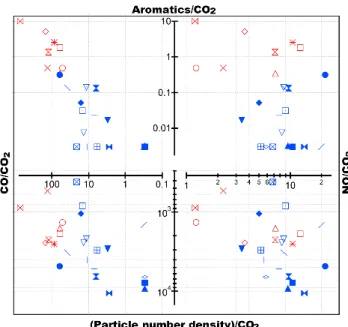
27 Figure 2. Comparison of emission ratios for CO/CO2 [ppb/ppm-CO2], NO/CO2 [ppb/ppm], fine (submicron) particle number density (PND/CO2) [particles/cm3/ppm], and aromatics/CO2 [ppb/ppm] (sum of benzene, toluene, C3-benzenes and C2-benzenes) of individual vehicles sampled in stationary mode for gasoline (red) and diesel (blue) vehicles.

Fig. 2. Comparison of emission ratios for CO/CO2[ppb/ppm-CO2], NO/CO2 [ppb/ppm], fine (submicron) particle number density (PND/CO2) [particles/cm3/ppm], and aromatics/CO2 [ppb/ppm] (sum of benzene, toluene, C3-benzenes and C2-benzenes) of indi-vidual vehicles sampled in stationary mode for gasoline (red) and diesel (blue) vehicles.

were targeted with the chase technique. Nevertheless, a num-ber of visibly high emission gasoline-powered vehicles were measured in chase mode, mostly pick-ups and vans, and the results are also included in Fig. 3 for comparison with mea-surements of emission ratios from HDDT vehicles.

3.3 Fleet average emission ratios

In addition to the chase technique, which focuses on a series of selected individual vehicles within a given vehicular class, fleet average on-road emissions can be obtained by process-ing randomly intercepted vehicle plumes from surroundprocess-ing traffic. During the fleet average mode the mobile laboratory measured on-road ambient air mixed with emissions of the surrounding vehicles under various driving modes. As de-fined in Zavala et al. (2006), we considered driving modes as “Stop and Go” (SAG) for situations when the mobile lab-oratory was in very heavy traffic conditions, with a vehicle fleet speed range of 16 (±8) km/h for 5 min or more; “Traf-fic” (TRA) for heavy traffic conditions with a vehicle fleet speed range of 40 (±16) km/h, for 5 or more minutes; and “Cruise” (CRU) for conditions with a moderate to high vehi-cle fleet speed of 56 km/h or higher, for 5 min or more. For these experimental settings, it is possible to obtain emission ratios classified by driving mode according to the predom-inant speed of the traffic. In addition, for measuring emis-sions under idling conditions (IDL) we used a semi “open-path” approach in which the mobile laboratory drives and

(7)

28 Figure 3. Mobile emission ratios measured from individual gasoline (red) and diesel (blue) vehicles. Each symbol represents an individual chased vehicle. “Aromatics” refers to the sum of benzene, toluene, C3-benzenes and C2-benzenes. “Particle number” [particles/cm3/ppm] refers to particle number density (PND). “Organics” refers to the organic component of the fine aerosol mass [ g/m3/ppm] less than 1 um in diameter. “Absorption” refers to PM light absorption [Mm-1/ppm]. All other units are in [ppb/ppm].

Fig. 3. Mobile emission ratios measured from individual gasoline (red) and diesel (blue) vehicles. Each symbol represents an individual

chased vehicle. “Aromatics” refers to the sum of benzene, toluene, C3-benzenes and C2-benzenes. “Particle number” [particles/cm3/ppm] refers to particle number density (PND). “Organics” refers to the organic component of the fine aerosol mass [µg/m3/ppm] less than 1 um in diameter. “Absorption” refers to PM light absorption [Mm−1/ppm]. All other units are in [ppb/ppm].

samples the emissions along a stationary or semi-stationary line of idling vehicles. The IDL mode measurements were predominantly obtained while sampling the line of vehicles waiting to cross the Mexican-US border between Mexicali and Calexico. In this experiment the mobile laboratory drove on a traffic-free road located beside the border crossing line, entering and re-entering several times, capturing idling and semi-idling emissions from the waiting vehicles.

In the fleet average mode, where even merged plumes from multiple vehicles can be processed and included, the sampling time (and therefore the number of vehicle exhaust plumes intercepted) is normally much larger than for chase mode measurements, providing better statistics. Success-ful application of this method requires a large sample size of mixed emission periods and long enough sampling times

so that the number of sampled vehicles is large enough to include a representative number of high emitters. Care must also be taken to avoid situations where the intercepted plumes are dominated by a few nearby vehicles for signifi-cant portions of the sampling period. On the basis of the cen-tral limit theorem, the emission averages should then be nor-mally distributed if the samples are unbiased and sufficiently large. In such case, symmetric confidence intervals around the average can be established for fleet emissions estimates. The emission ratios obtained in the fleet average operational sampling mode are appropriate to use for comparison with mobile emissions measured with other high sampling volume techniques and for the validation of an emissions inventory (Zavala et al., 2006).

(8)

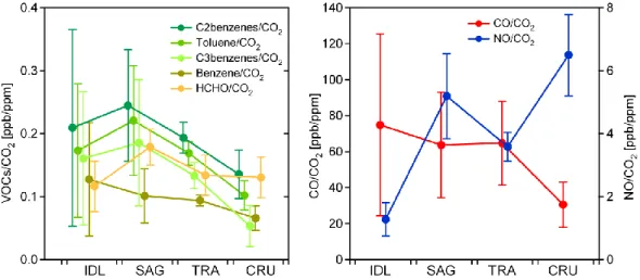
29 Figure 4. Fleet average mobile emission ratios by driving mode for CO/CO2, NO/CO2 and selected VOCs/CO2 showing the 75th, 50th, and 25th percentile for each driving mode.

Fig. 4. Fleet average mobile emission ratios by driving mode for CO/CO2, NO/CO2and selected VOCs/CO2showing the 75th, 50th, and 25th percentile for each driving mode.

The measured mobile emission ratios for gases and parti-cle properties sampled in fleet average mode are summarized in Table 1. Given that gasoline-fueled vehicles dominated the fleet characterized here and that our active filtering crite-ria excluded diesel plumes, the fleet average emissions mea-surements presented here represent the fleet of gasoline vehi-cles. Therefore, we will consider these measurements as rep-resentative of the gasoline-only fleet emission indices. Due to difficulties with inappropriate sampling frequency settings for the AMS instrument, there are no available fleet averaged emission PM species partitioning emission ratios for this op-erational sampling mode.

A more detailed view of the effect of driving speed on se-lected VOCs, NO and CO emissions is shown in Fig. 4. This figure shows the 75th, 50th, and 25th percentiles for selected VOCs, CO and NO emission ratios under the described driv-ing modes. Figure 4 clearly shows that the magnitude and variability of CO and VOCs, which are directly related to the combustion efficiency, are reduced with increasing speed whereas the variability of NO emission ratios does not de-crease at higher speeds. C2benzenes and benzene were the highest and lowest abundance aromatic species measured on a mole per mole basis.

Although the number of samples in some driving mode classifications is relatively small, this sampling technique is much more robust for obtaining fleet average emission con-ditions because their statistics are more significant than those from individual target vehicle emission measurements. Nev-ertheless, as shown in Table 1, most of the standard devia-tions are smaller than the observed average. The values re-ported in Table 1 are used in the following sections for the comparison with similar studies conducted in Mexico City.

4 Discussion

Quantification of emitted fine particles and specific gaseous pollutants often reveals large variability even within a given vehicle type, as indicated in Fig. 2. The measurement of in-dividual plumes in roadside stationary sampling showed that particle number density and NO emission ratios for HDDTs were, in general, higher than those for LDGVs. This is some-what expected but a larger variability is observed for NO emission ratios from LDGVs. The particularly large variabil-ity of NO emission ratios for LDGV may be the result of the different engine combustion temperatures regimes and the lack or malfunctioning of an emissions control system among the sampled vehicles (Wallington et al., 2006). Higher com-bustion temperatures lead to higher levels of thermal NOx (Zeldovich mechanism).

Results from the vehicle chase measurements in Mexicali (Fig. 3) also show generally higher CO and VOC emission ratios for high emitter gasoline-powered vehicles and high variability for almost all other measured parameters. Alde-hydes and other VOCs emission ratios are particularly high for these gasoline powered vehicles, a probable indication of the malfunctioning of, or the lack of, an emissions control system. Similarly, measured NO emission ratios for the high emitter gasoline vehicles are as large as the HDDT emission ratios. However, although the emitted VOCs are higher for the high emitter gasoline-powered vehicles, the organic con-tent in the particle phase of LDGVs still tends to be smaller than for HDDTs. This may partially be due to the higher content of low volatility hydrocarbon molecules in diesel as compared to gasoline fuels and to the better extent of the mixing state of the air/fuel (A/F) mixture in gasoline vehi-cles as compared to diesel (Wallington et al., 2006). Diesel emissions may also contain a larger fraction of unburned mo-tor oil (Canagaratna et al., 2004). Interestingly, the measured

(9)

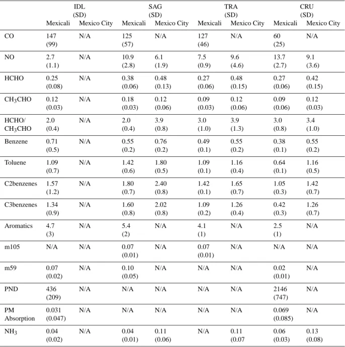
Table 1. Comparison of measured gasoline fleet-average mobile emission indices between Mexicali in 2005 and Mexico City in 2003 for

various driving modesa.

IDL SAG TRA CRU

(SD) (SD) (SD) (SD)

Mexicali Mexico City Mexicali Mexico City Mexicali Mexico City Mexicali Mexico City

CO 147 N/A 125 N/A 127 N/A 60 N/A

(99) (57) (46) (25) NO 2.7 N/A 10.9 6.1 7.5 9.6 13.7 9.1 (1.1) (2.8) (1.9) (0.9) (4.6) (2.7) (3.6) HCHO 0.25 N/A 0.38 0.48 0.27 0.48 0.27 0.42 (0.08) (0.06) (0.13) (0.06) (0.15) (0.06) (0.15) CH₃CHO 0.12 N/A 0.18 0.12 0.09 0.12 0.09 0.12 (0.03) (0.03) (0.06) (0.03) (0.06) (0.06) (0.03) HCHO/ 2.0 N/A 2.0 3.9 3.0 3.9 3.0 3.4 CH3CHO (0.4) (0.4) (0.8) (1.0) (1.3) (0.8) (1.0) Benzene 0.71 N/A 0.55 0.76 0.49 0.55 0.38 0.55 (0.5) (0.2) (0.2) (0.1) (0.2) (0.1) (0.2) Toluene 1.09 N/A 1.42 1.80 1.09 1.16 0.64 1.16 (0.7) (0.6) (0.5) (0.1) (0.4) (0.1) (0.5) C2benzenes 1.57 N/A 1.80 2.40 1.42 1.65 1.05 1.42 (1.2) (0.7) (0.8) (0.1) (0.7) (0.3) (0.7) C3benzenes 1.34 N/A 1.60 2.02 1.09 1.26 0.42 1.26 (0.9) (0.8) (0.8) (0.2) (0.4) (0.3) (0.7)

Aromatics 4.7 N/A 5.4 N/A 4.1 N/A 2.5 N/A

(3) (2) (1) (1)

m105 N/A N/A 0.07 N/A 0.07 N/A N/A N/A

(0.01) (0.01)

m59 0.07 N/A 0.10 N/A N/A N/A 0.02 N/A

(0.02) (0.05) (0.01)

PND 436 N/A N/A N/A N/A N/A 2146 N/A

(209) (747)

PM 0.031 N/A N/A N/A N/A N/A 0.069 N/A

Absorption (0.047) (0.085)

NH3 0.04 N/A 0.04 0.11 N/A 0.11 0.06 0.13

(0.02) (0.01) (0.06) (0.07 (0.03) (0.08)

a_{All units are in g pollutant/kg fuel except for particle number density (PND) [part/cc/ppm-CO}

2] and PM light absorption [1/um/ppm-CO2] and HCHO/CH3CHO [ppb/ppb]. We consider here C2Benzene as the sum of xylene isomers, ethylbenzene, and benzaldehyde and C3Benzene as the sum of C9H12isomers and C8H8O isomers. Aromatics are the sum of benzene, toluene, C3benzene and C2benzene. m105 and m59 generally refer to ion masses m/z signals that are related to ethylbenzene and acetone, respectively. IDL: idle; SAG: Stop and Go; TRA: Traffic; CRU: Cruise conditions. N/A: Not available, SD: 1 standard deviation. See text for details.

variability of the fine particle number density was similar in both types of vehicles but their light absorption, quantifying black carbon content, tends to be smaller for the gasoline ve-hicles. This is probably also a direct result of the different engine combustion process in the two vehicle classes.

Results from the gasoline fleet average measurements showed that NO, fine particle number density and CO emis-sion ratios varied significantly by driving mode whereas the effect is less evident for benzene and practically non-existent for HCHO emission ratios (Fig. 4). These effects of driving modes on emission ratios are consistent with results from

(10)

Mexico City using the same sampling technique (Zavala et al., 2006). Higher NO emission ratios for higher driving speeds are consistent with higher engine combustion tem-peratures and higher availability of oxygen in the combus-tion chamber of gasoline vehicles at those speeds (Kean at al., 2003; Jimenez et al., 1999). Similarly, the produc-tion of CO at low vehicle speeds increases as the A/F ra-tio decreases with less efficient combusra-tion (Fernandez, et al., 1997). Whereas NOxand CO are direct products of the combustion process, and therefore directly correlated with the A/F ratio or driving speed, the hydrocarbon emissions re-sult from a variety of other processes. These include blowby effects (leakage of gases escaping through sealing surfaces in the engine) during the compression and power strokes, evap-orative emissions (whose amount depends on the fuel volatil-ity, temperature and vehicle maintenance) and the combus-tion process itself. For these reasons, the hydrocarbon emis-sions result from a mixture of unburned fuel/oil and partially oxidized exhaust products. In general, fuel-based hydro-carbon emissions increase with heavy load conditions and higher power – that is, a rich A/F ratio (Kean et al., 2003).

As described above, there are a large number of factors that directly affect the emission characteristics of a given ve-hicle, all of which affect the observed variability during the sampling of on-road emissions. As such, it is of particular interest to compare the observed variability of the sampled plumes in roadside stationary mode, chase studies and fleet average emission ratios measurements. Comparison of emis-sion ratios obtained in different operational sampling modes provides an opportunity to understand the observed variabil-ity of the emission data.

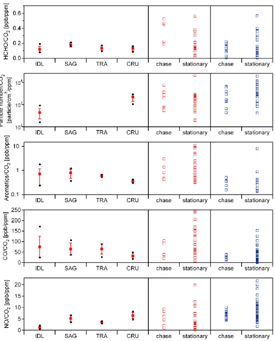
Figure 5 presents the 75th, 50th and 25th percentiles for the fleet average emission ratio measurements as well as all the emission ratios obtained from the chase and the road-side stationary sampling mode measurements of individual gasoline and diesel vehicles plumes. As described above, the four fleet average driving modes in Fig. 5 are more rep-resentative of the gasoline vehicle fleet with no significant representation of diesel vehicles. Figure 5 shows that there is higher variability in the sampling of individual plumes and chased vehicles than for the fleet average mode. Also, the variability of the measured emission ratios is larger for the individual plume samples than for the chase events for both gasoline and diesel vehicles. The higher variability of the roadside stationary individual sampled plumes and the chase modes can readily be explained by the “micro” approach of these measurement techniques where a large number of factors (emission control system, vehicle age, maintenance state, fuel type, etc.) may play a major role in determin-ing the emissions from a given vehicle. In the fleet average sampling mode, all these factors are smoothed by averaging (equally weighting) the measured emissions plumes. On the other hand, the variation observed in both the average and the standard deviation in the fleet average sampling mode indicates that the sampling size was large enough to be

sen-Table 2. Comparisons of gasoline fleet mobile emissions [tons/day]

in Mexicali (this study) with those estimated for other urban areas. (See comments in text).

Pollutant Mexicalia Imperial Valleya,b Mexico Cityc

CO 175±62 23 2765

NOx 10.4±1.3 2 188

Population 850 000 155 000 17 400 000 Vehicles 293 000 77 000 3 000 000 a_{Population and vehicle data from SEMARNAP (1999) projected} to 2005 using annual population grow rates of 2.6% and 1.5% as well as 2.9 and 1.9 persons per vehicle for Mexicali and the Imperial Valley, respectively.

b_{Emission data from CARB, (2007) for the 2005 light duty} passenger vehicles emissions for the Imperial Valley, CA.

c_{Data from the 2004 MCMA emissions inventory (CAM, 2006) for} LDGVs.

sitive to driving mode. Similarly, for emissions of CO, NO and some selected VOCs, the resulting consistently smaller standard deviations with respect to the observed emission ra-tio average in the fleet average mode and the (pronounced in some cases) variation observed with driving mode suggests that the sample size is adequate to represent a true average. This is of particular importance when the observed fleet av-erage emission ratios are used to estimate fuel-based total emission indices for the vehicle fleet, which, in turn, can be used to assess the validity of traditional “bottom up” emis-sions inventories (Singer and Harley, 2000). The validation of estimated mobile emission inventories is an important ap-plication of the measured mobile emission ratios.

Unfortunately, there was no available information on the local gasoline fuel sales or fuel consumption for Mexicali for the measurement period. However, as a first approxima-tion, we estimated the local gasoline sales by using the read-ily available national total fuel sales data for Mexico from PEMEX (the national petroleum company of Mexico) and scaled them by the number of vehicles in Mexicali compared to the national values (data which were readily available). This yielded estimated local fuel sales of 1 785 000 liters of gasoline per day for 2005. We focused on estimating fleet av-erage emissions because there was no data available to dis-aggregate these fuel sales by model year. To that end it is necessary to convert from ppb/ppm of CO2emitted to grams per liter of fuel consumed during the combustion process. We assume complete stoichiometric combustion, a typical value of 54.1 moles of carbon per liter of gasoline and a fuel den-sity of 756 grams/liter. This assumption is reasonably valid because the measured emissions levels of exhaust plume CO and VOCs are small compared to the levels of emitted CO2 (i.e. generally >90% of fuel carbon is emitted as CO2).

(11)

30 Figure 5. Comparison of measured on-road mobile emission ratios for various pollutants by sampling operational for gasoline (red) and diesel (blue) vehicles. “Aromatics” refers to the sum of benzene, toluene, C3-benzenes and C2-benzenes.

Fig. 5. Comparison of measured on-road mobile emission ratios for various pollutants by sampling operational for gasoline (red) and diesel

(blue) vehicles. “Aromatics” refers to the sum of benzene, toluene, C3-benzenes and C2-benzenes.

Using these assumptions we estimate the CO and NOx on-road emissions for Mexicali shown in Table 2. We compare the estimated gasoline mobile emissions in Mexicali with those from the neighbour Imperial Valley, CA (sharing the Mexico-US border with Mexicali) obtained from the Califor-nia Air Resources Board (CARB, 2007), and mobile emis-sions from Mexico City for light passenger vehicles obtained from the Metropolitan Environmental Commission (CAM, 2006). Mexicali CO emissions are larger than Imperial Val-ley by a factor of 8, whereas NOx emissions are larger by a factor of about 6. The fleet size in Mexicali compared to the Imperial Valley is a factor of about 4 higher indicating

that on a vehicle-per-vehicle basis the fleet in Mexicali is 1.4 to 2 times more polluting, probably due to difference in the fleet age (SEMARNAP, 1999). Detailed explanations of the differences between the measurement-based and the model-based emissions estimates are outside the scope of this paper. Nevertheless, an important consideration is that a large num-ber of vehicles cross back-and-forth between the two cities daily, and all are emitting into a shared air basin.

In Table 1, we also compare the gasoline vehicle fleet emission ratios measured during the Mexicali campaign with those obtained in Mexico City during the MCMA-2003 field campaign (Molina et al., 2007). In both campaigns the ARI

(12)

mobile laboratory obtained the on-road emission measure-ments using the same techniques, instrumentation and analy-sis procedures. As such, differences in the reported emission ratios reflect more directly the differences in fleet character-istics and composition between the two urban areas rather than differences in instrumentation, measurement techniques or data analysis procedures. We do not report CO emission ratios for Mexico City because the response time of the CO instrument used during the MCMA-2003 field campaign was not fast enough to fully resolve individual emission plumes.

On average, Mexico City measurements were made at higher relative humidity and lower temperature (45%, 19◦C) conditions than Mexicali measurements (28%, 24◦C) dur-ing the respective sampldur-ing periods. Higher humidity typi-cally results in lower NOxemissions whereas higher temper-atures would increase emissions. However, these differences in ambient conditions between the two cities are not large enough to explain the observed differences. A major differ-ence between the two cities is the nominal ambient pressure (76 kPA for Mexico City versus 100 kPA for Mexicali). Un-fortunately, there is little information in the archival literature about the effects of altitude on gasoline fueled vehicles. At high altitude, the air-fuel ratio supplied to the engine may be reduced because air density is reduced. With a richer air-fuel mixture, un-burnt components in the exhaust increase. However, although gasoline emissions in Mexico City would in principle tend to be higher than in Mexicali because of the higher altitude, modern gasoline vehicles are generally provided with mechanisms that compensate for the effect of altitude on air density, minimizing this effect. Manufacturers conduct certification testing in the laboratory (for example by restricting the flow of air to the engine intake and equal-izing intake and exhaust pressures) to comply with on-road standards for regulated emissions.

Interesting differences can be found in the emissions data between the two cities. NO emission ratios are ∼20% higher in Mexicali than in Mexico City whereas HCHO emission ratios are higher by almost a factor of 2 in Mexico City. However, emission ratios of acetaldehyde in Mexicali do not seem to be significantly different from those in Mexico City, hence the corresponding HCHO/CH3CHO ratio varies with the HCHO emission ratio. The elevated HCHO emissions in Mexico City are particularly important since photolysis of HCHO produces HOx radicals, which initiate tropospheric ozone production and secondary aerosol formation.

Aromatic species emission ratios measured in the Mexicali gasoline vehicle fleet are slightly, but consistently, smaller than those measured in Mexico City. Nevertheless, the vari-ability in the selected VOCs emission ratios seems to be higher in the Mexico City measurements and the difference may not be statistically significant. The variability may be due to the difference in the sampling size (almost a factor of 4 higher in Mexico City) between the two experimental settings. Emission ratios of NH3also seem to be higher in Mexico City than in Mexicali by a factor of 2 or more. In

general, higher VOC and NH3 emission ratios are seen in Mexico City possibly due to more prevailing fuel-rich con-ditions induced by Mexico City’s much higher altitude and lower ambient oxygen concentration per volume of air.

Remote sensing studies in Mexico City and Monterrey, Mexico in the early 1990’s showed average light-duty ve-hicle emission factors of about 181 g/kg and 19 g/kg for CO and NO, respectively (Bishop et al., 1997). At that time new emission standards had just been introduced in Mexico and a large fraction of the fleet had no catalytic converters, result-ing in large fuel-based emission factors. A comparison of vehicle emission factors in Table 1 with studies in US cities (e.g. Ban-Weiss et al., 2008; Bishop and Stedman, 2008) shows that the vehicle fleets from both Mexican cities gen-erally have much higher fuel-based emission factors. In the late 1990s mean emission factors from light-duty vehicles in several US cities ranged from 40–70 g/kg for CO and from 5–9 g/kg for NO, following a continuously decreasing trend (Harley et al., 2005; Bishop and Stedman, 2008). CO and NO emission factors measured in Mexicali (60–147 g/kg and 2.7–13.7 g/kg, respectively) are within the ranges of mea-surements of the late 1990s in US cities, and lower than those measured in Mexico City and Monterrey in the early 1990’s. The variability of the NO and selected VOCs emission ra-tios with respect to driving mode seems to be consistent in both datasets although a bit more pronounced in Mexicali than in Mexico City, particularly at cruising speeds. Among the major factors that may play a role in explaining the ob-served differences between the two measurements are the fleet age, the distribution of vehicle types, the fraction of ve-hicles with emission control technology and the fuel compo-sition. For example, using the base year of 1999 for the com-parison, the vehicle fleet in Mexicali was on average more than 7 years older and the fraction of vehicles without some emission control technology was about twice that in Mexico City (SEMARNAP, 1999). Other local parameters that may play a role in the differences between the emissions measured in the two urban areas are the temperature, altitude (ambi-ent pressure) and to some ext(ambi-ent the relative humidity. In a rapidly growing urban zone such as the US-Mexico border, the vehicle fleet size and fuel consumption are continuously changing, effectively making the estimation of mobile emis-sions a moving target. As mobile emisemis-sions clearly play an important role in the formation of ozone and secondary or-ganic aerosols in urban areas, it would be of major interest to design a follow up study aimed at exploring in detail each of these factors and parameters influencing the differences be-tween the two cities and their correlation with ambient pol-lution levels.

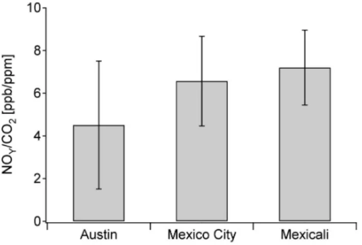
The measurements of on-road NOy emission ratios in Austin for individual HDDTs sampled in chase mode are presented in Fig. 6 ordered by average driving speed. The on-road emission measurements of the trucks, which were identified by recording their license plates, occurred mostly on an isolated highway at moderate to high speeds. The

(13)

31 Figure 6. Average NOy/CO2 on-road emission ratios of individual HDDTs measured in Austin

TX, colored by vehicle speed.

Fig. 6. Average NOy/CO2 on-road emission ratios of individual HDDTs measured in Austin TX, colored by vehicle speed.

results indicate a large variability of NOyemission ratios be-tween individual vehicles as a function of average vehicle speed. The observed variability correlated with vehicle speed may also be an indication of enhanced thermal NOx forma-tion at higher engine temperatures. We compare the diesel NOy on-road emission ratios from individual HDDTs mea-sured in chase mode in Mexico City, Mexicali and Austin (see Fig. 7). Bishop et al. (2001) report an increase in emis-sions with altitude from diesel vehicles. Our results show lower NOy emissions in Mexico City than in Mexicali de-spite the observed altitude effect, implying that other effects on NOy emissions (e.g. vehicle age and driving mode) are larger. Because NO emissions from heavy-duty diesel ve-hicles tend to be normally distributed, smaller data sets can be used to obtain meaningful averages (Bishop et al., 2001). Still, these measurements represent emissions from a very limited number of vehicles and it is possible that the sample size is not sufficient to produce fleet average HDDT emission ratios. Nevertheless, within the limitations of the sample size of our data, Fig. 7 indicates that on average NOy emission ratios from HDDTs in Mexicali and the MCMA were higher than those in Austin and that the variability (indicated here as the 1-sigma standard deviation of the measurements) is sim-ilar in all three locations. The large variability observed in the NOyemission ratios is likely due to the large number of parameters affecting HDDT emissions.

5 Conclusions

We have applied the measurement technique for on-road mo-bile emission developed in the Mexico City Metropolitan Area during the MCMA-2003 Campaign to Mexicali as part of the BORAQIP program for the Mexicali-Imperial Valley in 2005 and compare similar on-road emission ratios from the two cities. Similar to Mexico City, the measurements in Mexicali were obtained under different driving modes representing various speed and traffic characteristics of the

32 Figure 7. Comparison of on-road NOy/CO2 emission ratios measured in Austin, Mexicali and

Mexico City for HDDTs. The error bars represent the 1 standard deviation of the data.

Fig. 7. Comparison of on-road NOy/CO2emission ratios measured in Austin, Mexicali and Mexico City for HDDTs. The error bars represent the 1 standard deviation of the data.

fleet and using three different operational sampling modes – roadside stationary sampling, chase studies and fleet average measurements. The analysis focused on the magnitude and variability of the measured emission ratios under different operational sampling modes.

The observed variability increased from fleet average to chase and roadside stationary sampling for all measured gases and particle emission ratios. The high variability ob-served in roadside stationary sampling and chase studies can be explained by the large number of factors that can deci-sively impact the emissions from a given vehicle. The fleet average sampling mode captured the effects of driving con-ditions on the measured on-road emission ratios. This is im-portant because the measured on-road emission ratios can be used to estimate fuel-based emission indices used, in turn, to asses the validity of traditional “bottom-up” emissions in-ventories. Scaling national fuels sales data for Mexicali, we estimated CO and NOxemissions of 175±62 and 10.4±1.3 metric tons/day, respectively, for the gasoline vehicle fleet. These emissions are 8 and 6 times larger than the emissions estimated for Imperial Valley, CA (the US neighbour county) due in part to the much larger fleet size in Mexicali.

Comparisons with similarly obtained on-road emissions data in Mexico City indicated that NO emission ratios were around 20% higher in Mexicali than in Mexico City whereas HCHO and NH3 emission ratios were higher by a factor of 2 in Mexico City. Acetaldehyde emission ratios were not significantly different in the two Mexican cities. Aro-matic species emission ratios were similar to or smaller in Mexicali. Differences in reported emission ratios di-rectly reflect the differences in fleet characteristics between the two cities, rather than differences in instrumentation, measurement technique or driving and operational sampling modes. Measurements of NOyemission ratios from individ-ual chased HDDTs in Austin showed a strong correlation

(14)

with vehicle speed, similar to the results in Mexicali and Mexico City. However, comparison of the NOyemission ra-tios from HDDTs obtained in the three cities showed that, on average, NOyemission ratios from HDDTs in Mexicali were higher than in Mexico City, but the ratios from both Mexi-can cities were higher than in Austin; the variability of the measurements was similar in all three locations.

Acknowledgements. The authors gratefully acknowledge the financial support from the Mexican Metropolitan Environmental Commission (CAM) and the US National Science Foundation (ATM-0528227) for the Mexico City measurements, LASPAU Border Ozone Reduction and Air Quality Improvement Program for the Mexicali measurements, and the University of Texas and the Molina Center for the Energy and the Environment for the Austin measurements. Mobile laboratory operational support was provided by Centro Nacional de Investigación y Capacitación Ambiental (CENICA) in Mexico City, Universidad Autónoma de Baja California (UABC) in Mexicali, and the University of Texas in Austin.

Edited by: U. P¨oschl

References

Andr´e, M., Joumard, R., Vidon, R., Tassel, P., and Perret, P.: Real-world European driving cycles, for measuring pollutant emis-sions from high- and low-powered cars, Atmos. Environ., 40, 5944–5953, 2006.

Ban-Weiss, G., McLaughlin, J., Harley, R., Lunden, M., Kirchstet-ter, T., Kean, A., Strawa, A., Stevenson, E., and Kendall, G.: Long-term changes in emissions of nitrogen oxides and partic-ulate matter from on-road gasoline and diesel vehicles, Atmos. Environ., 42, 220–232, 2008.

Bishop, G., Stedman. D., de la Garza, J., and D´avalos, F.: On-road remote sensing of vehicle emissions in Mexico, Environ. Sci. Technol., 31, 2, 3505–3510, 1997.

Bishop, G., Morris, J., Stedman, D., Cohen, L., Countess, R., Countess, S., Maly, P., and Scherer, S.: The effects of altitude on heavy-duty diesel truck on-road emissions, Environ. Sci. Tech-nol., 35, 8, 1574–1578, 2001.

Bishop, G. and Stedman, D.: A decade of on-road emissions mea-surements, Environ. Sci. Technol., 42, 5, 1651–1656, 2008. Cadle, S. H., Ayala, A., Black, K. N., Fulper, C. R., Graze, R. R.,

Minassian, F., Natarajan, M., Tennant, C. J., and Lawson, D. R.: Real-world vehicle emissions: a summary of the Sixteenth Co-ordinating Research Council On-Road Vehicle Emissions Work-shop, J. Air Waste Manage., 57(2), 139–145, February, 2007. CAM (Comisi´on Ambiental Metropolitana): Inventario de

emi-siones 2004 de la Zona Metropolitana del Valle de México, Sec-retar´ıa del Medio Ambiente, Gobierno de México, México, avail-able from http://www.sma.df.gob.mx/, 2006.

Canagaratna, M. R., Jayne, J. T., Ghertner, D. A., Herndon, S. C., Shi, Q., Jimenez, J. L., Silva, P. J., Williams, P., Lanni, T., Drewnick, F., Demerjian, K. L., Kolb, C. E., and Worsnop, D. R.: Chase Studies of Particulate Emissions from in-use New York City Vehicles, Aerosol Sci. Tech., 38, 555–573, 2004.

CARB (California Air Resources Board): 2006 Almanac emission projection data, available from http://www.arb.ca.gov/, 2007. Chan, T., Ning, Z., Leung, C., Cheung, C., Hung, W., and Dong, G.:

On-road remote sensing of petrol vehicle emissions measurement and emission factors estimation in Hong Kong, Atmos. Environ., 38, 2055–2066, 2004.

Cicero Fernandez, P., Long, J. R., and Winer, A. M.: Effects of grades and other loads on on-road emissions of hydrocarbons and carbon monoxide, J. Air Waste Manage., 47, 898–904, 1997. Dong, G. and Chan, T. L.: Large eddy simulation of flow structures

and pollutant dispersion in the near-wake region of a light-duty diesel vehicle, Atmos. Environ., 40, 1104–1116, 2006.

Durbin, T., Johnson, K., Miller, J., Maldonado, H., and Chernich, D.: Emissions from heavy-duty vehicles under actual on-road driving conditions, Atmos. Environ., 42, 4812–4821, 2008. Harley, R., Marr, L., Lehner, J., and Giddings, S.: Changes in motor

vehicle emissions on diurnal to decadal time scales and effects on atmospheric composition, Environ. Sci. Technol., 39, 5356– 5362, 2005.

Herndon, S. C., Jayne, J. T., Zahniser, M. S., Worsnop, D. R., Knighton, B., Alwine, E., Lamb, B. K., Zavala, M., Nelson, D. D., McManus, J. B., Shorter, J. H., Canagaratna, M. R., Onasch, T. B., and Kolb, C. E.: Characterization of urban pollutant emis-sion fluxes and ambient concentration distributions using a mo-bile laboratory with rapid response instrumentation, Faraday Dis-cuss., 130, 327–339, 2005.

Herndon, S. C., Shorter, J. H., Zahniser, M. S., Nelson, D. D. J., Jayne, J. T., Brown, R. C., Miake-Lye, R. C., Waitz, I. A., Silva, P., Lanni, T., Demerjian, K. L., and Kolb, C. E.: NO and NO2 emission ratios measured from in-use commercial aircraft during taxi and takeoff, Environ. Sci. Technol., 38, 6078–6084, 2004. Jimenez, J. L., Koplow, M. D., Nelson, D. D., Zahniser, M. S., and

Schmidt, S. E.: Characterization of on-road vehicle NO emis-sions by a TILDAS remote sensor, J. Air Waste Manage., 49, 463–470, 1999.

Joumard, R., Andr´e, M., Vidon, R., Tassel, P., and Pruvost, C.: In-fluence of driving cycles on unit emissions from passenger cars, Atmos. Environ., 34, 4621–4628, 2000.

Kean, A. J., Harley, R. A., and Kendall, G. R.: Effects of vehicle speed and engine load on motor vehicle emissions, Environ. Sci. Technol. 37, 3739–3746, 2003.

Kolb, C. E., Herndon, S. C., McManus, J. B., Shorter, J. H., Zah-niser, M. S., Nelson, D. D., Jayne, J. T., Canagaratna, M. R., and Worsnop, D. R.: Mobile laboratory with rapid response instru-ments for real-time measureinstru-ments of urban and regional trace gas and particulate distributions and emission source characteristics, Environ. Sci. Technol., 38, 5694–5703, 2004.

Mendoza, A., Kolb, C., and Russell, A. G.: Mexicali-Imperial val-ley air quality modeling and monitoring program, final report prepared for LASPAU’s Border Ozone Reduction and Air Qual-ity Improvement Program, 1–50, January, 2007.

Molina, L. T., Kolb, C. E., de Foy, B., Lamb, B. K., Brune, W. H., Jimenez, J. L., Ramos-Villegas, R., Sarmiento, J., Paramo-Figueroa, V. H., Cardenas, B., Gutierrez-Avedoy, V., and Molina, M. J.: Air quality in North America’s most populous city – overview of the MCMA-2003 campaign, Atmos. Chem. Phys., 7, 2447–2473, 2007,

http://www.atmos-chem-phys.net/7/2447/2007/.

(15)

Meng, F., Singh, R. B., Galvez, O., Sloan, J. J., Anderson, W. P., Tang, X. Y., Hu, M., Xie, S., Shao, M., Zhu, T., Zhang, Y. H., Gurjar, B. R., Artaxo, P. E., Oyola, P., Gramsch, E., Hidalgo, D., and Gertler, A. W.: Air quality in selected megacities, critical review complete online version, http://www.awma.org, 2004. NARSTO: Improving emissions inventories for effective air

qual-ity management across North America, a NARSTO assessment, NARSTO-05-001, 2005.

Ntziachristos, L. and Samaras, Z.: Speed-dependent representative emission factors for catalyst passenger cars and influencing pa-rameters, Atmos. Environ., 34, 4611–4619, 2000.

Pierson, W., Gertler, A., Robinson, N., Sagebiel, J., Zielinska, B., Bishop, G., Stedman, D., Zweidinger, R., and Ray, W.: Real-world automotive emissions-Summary of studies in the Fort McHenry and Tuscarora mountain tunnels, Atmos. Environ., 30, 2233–2256, 1996.

SEMARNAP: Programa para mejorar la calidad del aire de Mex-icali, 2000–2005, Secretaria de Medio Ambiente, Recursos Naturales y Pesca (SEMARNAP), available from http://www. semarnat.gob.mx/, 1999.

Shah, S., Johnson, K., Miller, J., and Cocker III, D.: Emission rates of regulated pollutants from on-road heavy-duty diesel vehicles, Atmos. Environ., 40, 147–153, 2006.

Singer, B. C. and Harley, R. A.: A fuel-based inventory of motor ve-hicle exhaust emissions in the Los Angeles area during summer 1997, Atmos. Environ., 34, 1783–1795, 2000.

Sjodin, A. and Lenner, M.: On-road measurements of single vehicle pollutant emissions, speed and acceleration for large fleets of ve-hicles in different traffic environments, Sci. Total Environ., 169, 1–3, 1995.

Tong, H. and Hung, W.: On-road motor vehicle emissions and fuel consumption in urban driving conditions, J. Air Waste Manage., 50, 543–554, 2000.

Wallington, T. J., Kaiser, E. W., and Farrell, J. T.: Automotive fuels and internal combustion engines: achemical perspective, Chem. Soc. Rev., 35, 335–347, 2006.

Walsh, P. A., Sagebiel, J. C., Lawson, D. R., Knapp K. T., and Bishop, G. A.: Comparison of auto emission measurement tech-niques, Sci. Total Environ., 189, 175–180, 1996.

Wang, J. S., Chan, T. L., Cheung, C. S., Leung, C. W., and Hung, W. T.,: Three-dimensional pollutant concentration dispersion of a vehicular exhaust plume in the real atmosphere, Atmos. Environ., 40, 484–497, 2006.

Zavala, M., Herndon, S. C., Slott, R. S., Dunlea, E. J., Marr, L. C., Shorter, J. H., Zahniser, M., Knighton, W. B., Rogers, T. M., Kolb, C. E., Molina, L. T., and Molina, M. J.: Characterization of on-road vehicle emissions in the Mexico City Metropolitan Area using a mobile laboratory in chase and fleet average measure-ment modes during the MCMA-2003 field campaign, Atmos. Chem. Phys., 6, 5129–5142, 2006,