HAL Id: hal-01411119
https://hal.inria.fr/hal-01411119
Submitted on 7 Dec 2016
HAL is a multi-disciplinary open access
archive for the deposit and dissemination of
sci-entific research documents, whether they are
pub-lished or not. The documents may come from
teaching and research institutions in France or
abroad, or from public or private research centers.
L’archive ouverte pluridisciplinaire HAL, est
destinée au dépôt et à la diffusion de documents
scientifiques de niveau recherche, publiés ou non,
émanant des établissements d’enseignement et de
recherche français ou étrangers, des laboratoires
publics ou privés.
Expert-based on-line learning and prediction in Content
Delivery Networks
Nesrine Ben Hassine, Dana Marinca, Pascale Minet, Dominique Barth
To cite this version:
Nesrine Ben Hassine, Dana Marinca, Pascale Minet, Dominique Barth. Expert-based on-line
learn-ing and prediction in Content Delivery Networks. IWCMC 2016 - The 12th International
Wire-less Communications & Mobile Computing Conference, Sep 2016, Paphos, Cyprus. pp.182 - 187,
�10.1109/IWCMC.2016.7577054�. �hal-01411119�
Expert-based On-line Learning and Prediction in
Content Delivery Networks
Nesrine Ben Hassine
∗†, Dana Marinca
†∗, Pascale Minet
∗, Dominique Barth
†∗Inria Paris, 2 rue Simone Iff, CS 42112, 75589 Paris Cedex 12,
Email: [email protected], [email protected]
†DAVID, University of Versailles, Versailles, France,
Email: [email protected], [email protected]
Abstract—Machine learning techniques can be used to improve the quality of experience for the end users of Content Delivery Networks (CDNs). In a CDN, the most popular video contents are cached near the end-users in order to minimize the contents delivery latency. The idea developed hereafter consists in using prediction techniques to evaluate the future popularity of video contents in order to decide which should cached. We consider various prediction methods, called experts, coming from different fields (e.g. statistics, control theory). We assess these experts ac-cording to three criteria: cumulated loss, maximum instantaneous loss and best ranking. We also show the importance of a decision maker, called forecaster, that predicts the popularity based on the predictions of selection of several experts. The forecaster based on the best K experts outperforms in terms of cumulated loss the individual experts’ predictions and those of the forecaster based on only one expert, even if this expert varies over time.
I. INTRODUCTION
Content Delivery Networks (CDNs) have undergone an ever-increasing success, leading to an important increase in multimedia traffic that could result in unacceptable delays for the mobile or fixed end users. The user mobility strongly impacts the solicited caches: their content should be updated dynamically to reflect users’ solicitations. To mitigate this effect, caching techniques are used in nodes near the end users. Hence, to decide which video contents should be cached is a challenging task that requires an in-depth analysis of the popularity of video contents over time.
In this paper, we focus on the use of machine learning techniques in CDNs. The remainder of this paper is organized as follows. In this section, we present the context of this study and some related work. In Section II, we define the theoretical framework including the problem statement. In the context of our paper, an expert refers to a software component that implements a prediction computation method. We define all the experts used (e.g. DES, Basic, polynomial or Savitzky-Golay regression, etc) coming from various fields (e.g. statistics, control theory) and explain how they compute their predictions. These predictions are used by a decision maker, called forecaster, to build its own prediction. We define two types of forecasters: Best Expert (BE) and K Best Experts (KBE). In Section III, we report our simulation results obtained from real traces of YouTube. We consider various video contents and evaluate the prediction accuracy of the forecasters and experts considered. We also compare the
experts using multiple criteria (e.g. cumulated loss, maximum instantaneous loss, best ranking). Finally, Section IV gives the conclusion.
A. Context
Our goal is to predict the popularity of video content in a CDN. As in many other studies [1], [2], [3], [4], we evaluate the popularity of a video content by its number of solicitations over a period of time. Hence, we predict the video content popularity by approximating the function representing the evolution of the number of solicitations over time.
For that purpose, we will evaluate different prediction methods applied on the same data extracted from real traces of YouTube CDN. We adopt the following approach where the popularity prediction is made in two steps. In the first step, each expert computes its prediction using its own prediction strategy (e.g. average, regression, exponential smoothing). In a second step, the forecaster uses the predictions given by the experts to build its own prediction. Here again, different strategies are possible. For instance, the forecaster may select the best expert or a group of best experts. Having selected its group of experts, the forecaster may use averaging or voting techniques. The best experts are those that provide the most accurate predictions. The accuracy of predictions is evaluated by the cumulated gap between the prediction and the real value up to current time. We will first justify the choice of this two-step approach based on experts and forecasters.
B. Related work
Let us consider a dynamic system whose parameters often change over time. We consider an online prediction problem where system is observed at different times and there is a challenge of maximizing prediction accuracy. This problem occurs in a multitude of machine learning applications.
Gu and Wang [5] use on-line prediction in a data stream processing application. They combine Markov models and Bayesian classification methods to predict the bottleneck that could appear, and its probable cause, while clustering data streams.
Many studies have used on-line prediction to deal with the limited battery lifetime problem. In [6], the authors employ a statistical approach to predict online the battery lifetime for embedded and mobile devices. They incorporate both recently
observed power dissipation values with pre-computed off-line reference signature. The battery lifetime prediction [8] is based on the usage patterns of individual users. Furthermore, in [7] an online approach is used during runtime to identify whether a failure will occur in the near future based on the monitored current system state.
In a previous study [9], we applied on-line prediction to predict the quality of links in a wireless sensor network. We combined a range of learning techniques and we identified the best parameter tuning of these techniques which provides a better approximation of the real values of the quality of the links.
II. THEORETICAL FRAMEWORK
A. Problem statement
From YouTube platform, we extract the real traces describ-ing the daily solicitation evolution over time of randomly chosen video contents. We consider that the number of so-licitations defines the popularity of a video content. We then focus on any video content among the selected ones. Based on its daily solicitations in the time interval [0, t], the goal is to predict its popularity during the day t + 1.
The prediction model is based on a set of experts, each expert being a logical entity which computes and predicts the future number of solicitations for each video content using its own computation method (Section II-B). A special expert, called forecaster, predicts the number of solicitations based on a selection of best expert predictions (Section II-D). We will show that forecaster predictions are more accurate than individual experts predictions (Section III-B).
Let us introduce some notations:
• {Ei, i ≥ 1} the set of experts.
• owi the observation window of expert Ei.
• {Fj, j ≥ 1} the set of forecasters.
For any given video content:
• ytthe number of solicitations at time t.
• pi,t the prediction of the expert Ei for time t.
• pˆj,t the prediction of the forecaster Fj for time t.
B. Experts definition
The prediction methods used by the proposed experts come from statistics or control theory. These prediction methods are based on exponential smoothing [10], average of corrections, regression [11] or filtering [12].
1) Double Exponential Smoothing (DES) Expert:
The DES expert [10], uses exponential smoothing to compute
its prediction. A DES expert Ei applies the exponential
smoothing twice: first on yt to compute S
0
i,t and second on
S0i,tto compute Si,t00. Both smoothings use the same smoothing factor α with 0 < α < 1,
Si,00 = Si,000 = y0.
Si,t0 = αyt+ (1 − α)S 0 i,t−1.
Si,t00 = αSi,t0 + (1 − α)Si,t−100 .
At time t, the DES expert Ei predicts the value
pi,t+1 = Li,t+ Ti,t (1)
where Li,t= 2S
0 i,t− S
00
i,t denotes the estimated level
and Ti,t=1−αα (S 0 i,t− S
00
i,t) the estimated trend.
2) Constant Basic (CB) expert:
The Constant Basic (CB) expert has been defined in [13]. The
expert Ei predicts at time t the value for time t + 1 given by:
pi,t+1= yt+ ci∗ (yt− yt−1) (2)
where ci denotes the correction coefficient. In this prediction
method, ci is fixed.
3) Dynamic Basic (DB) expert:
The Dynamic Basic (DB) expert Ei uses the same prediction
method as the previously defined one, except that the correc-tion coefficient is computed dynamically as follows:
ci,t=
yt− yt−1
yt−1− yt−2
. (3)
4) Arithmetical Moving Average (AMA) adjusted expert: The Arithmetical Moving Average (AMA) adjusted expert,
Ei predicts a value that is adjusted using a coefficient equal
to the arithmetical average of dynamic correction coefficients over the solicitation values in its observation window ow. |ow| represents the number of values in ow.
pi,t+1= yt+ ¯ci,t∗ (yt− yt−1) (4)
with ¯ci,t =
P
k∈owci,k
|ow| , where ci,k is computed according to
Equation 3.
5) Geometrical Moving Average (GMA) adjusted expert:
The Geometrical Moving Average (GMA) adjusted expert, Ei
predicts a value that is adjusted using a coefficient equal to the geometrical average of dynamic correction coefficients over its observation window ow.
pi,t+1= yt+ ¯ci,t∗ (yt− yt−1) (5)
with ¯ci,t= |ow|pQk∈owci,k, where ci,kis computed according
to Equation 3.
6) Polynomial Regression (PR) expert:
The Polynomial Regression (PR) experts smooth the time function to approximate the real profile, by an n-degree poly-nomial extrapolation. Given n the degree of the polypoly-nomial,
the coefficients ak, k ∈ [0, n] involved in the regression are
calculated in such a way that they fit the relationship among data in the observation window ow. At time t, the Polynomial
Regression expert Ei predicts the value:
7) Savitzky Golay (SG) regression expert:
Savitzky Golay (SG) regression experts smooth the time function of the real profile by a Savitzky Golay filter. The idea of the Savitzky Golay filter is to find the set of coefficients
a0, . . . , an which best preserve the shape of the features
present in the sampled profile. The approach is to make a polynomial regression of the observations in the window ow around its center k, and then evaluate this polynomial at time
k + |ow/2| + 1. The coefficients al, with l ∈ [0..n], involved
in the regression are computed by a convolution of the input data in ow with the coefficient vector given by Equation 7.
al= |ow|/2 X j=−|ow|/2 vjyj (7) pi,t+1= a0+ a1(t − k) + . . . + an(t − k)n (8)
The observation window size |ow| should be odd and greater than n the degree of the polynomial.
The arithmetical average smoothing corresponds to the case where all coefficients al, with l ∈ [0, n] are equal to 1/|ow|.To
determine the smoothed value for each data point, the local polynomial regression is better than adjacent averaging be-cause it tends to preserve features of the data such as peak height and width, which are usually eliminated by adjacent averaging.
C. Accuracy of an expert
The prediction accuracy of an expert Ei is evaluated by
its loss regarding the gap between its prediction and the real solicitation value. We define several types of losses for any
expert Ei, computed at each time instant t:
• the instantaneous loss, denoted li,t, meets:
li,t= |yt− pi,t|;
• the cumulated loss, denoted Li,t, satisfies:
Li,t = t X k=1 |yk− pi,k| = t X k=1 li,k;
• the maximum instantaneous loss, denoted lmaxi,t, meets:
lmaxi,t= maxk∈[0,t]li,k.
D. Forecasters definition
At each time t, a forecaster selects some experts that minimize their cumulated loss and computes a prediction value based on the selected experts predictions. We propose two types of forecaster.
1) Best Expert (BE) forecaster:
At each time t, the BE forecaster Fjselects exactly one expert
Ei that minimizes the cumulated loss. The forecaster predicts
the value predicted by the selected expert Ei.
2) K Best Experts (KBE) forecaster:
At each time t, a KBE forecaster Fj selects the experts
that provide the K smallest cumulated losses. The forecaster predicts the average of the predictions given by those best experts. Notice that since several experts may predict the same value, the forecaster may select more than K best experts. E. Accuracy of a forecaster
Similarly, the accuracy of a forecaster Fj is evaluated by
the gap between its prediction and the real solicitation value at each time instant t. We define several types of losses for any forecaster Fj:
• the instantaneous loss, denoted ˆlj,t, meets:
ˆ
lj,t= |yt− ˆpj,t|; • the cumulated loss, denoted ˆLj,t, satisfies:
ˆ Lj,t= t X k=1 |yk− ˆpj,t| = t X k=1 ˆ lj,t;
• the maximum instantaneous loss, denotedlmaxˆ j,t, meets:
ˆ
lmaxj,t= maxk∈[0,t]ˆlj,k.
F. Algorithm of a KBE forecaster
The algorithm of the KBE forecaster is given by Algo-rithm 1. To begin, the forecaster computes its instantaneous loss and its cumulated loss. The forecaster is allowed to see the losses and the predictions of all experts. At each time t, it
observes the Kth smallest cumulated loss among all expert
cumulated losses. It selects the experts having at time t a cumulated loss less than or equal to the observed cumulated loss and constitutes its group of best experts. Subsequently, it computes the average of the predictions of its best experts and predicts this value.
We can notice that the BE forecaster can be considered as a specific case of a KBE forecaster, where exactly one expert is chosen among those providing the minimum cumulated loss. Algorithm 1 KBE Forecaster’s algorithm at time t > 0
ˆ
lj,t= |ˆpj,t− yt|
ˆ
Lj,t= ˆLj,t−1+ ˆlj,t
Selected Experts = ∅
Sort the experts by increasing Li,t
Last cumul = the Kth value f or the cumulated loss
ˆ pj,t= 0
for i ∈ [1, n] do
if Li,t≤ Last cumul then
Selected Experts = Selected ExpertsS{Ei}
ˆ pj,t= ˆpj,t+ pi,t end if end for ˆ pj,t= ˆpj,t/size(Selected Experts)
III. SIMULATION RESULTS A. Real traces
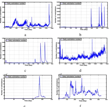
In this study, we extracted from YouTube platform, real traces describing the daily solicitation evolution over time of randomly chosen video contents. The daily solicitations concern the period from the instant of the online availability up to the current time. We then focus on any video content among the selected ones. Knowing its daily number of solicitations in the time interval [0, t], the goal is to predict how many times this content will be solicited during the day t + 1.
Figure 1 depicts the evolution of solicitations day by day for different video content profiles used in our tests. We observe that, during the lifetime of these contents, they have totally different profiles of solicitations: order of magnitude and evolution curve of solicitations.
0 200 400 600 800 1000 1200 1400 1600 0 200 400 600 800 1000 Time (Day) Number of solicitations
Daily solicitation number
a 0 50 100 150 200 250 300 350 400 450 0 2000 4000 6000 8000 10000 12000 14000 16000 Time (Day) Number of solicitations
Daily solicitation number
b 0 20 40 60 80 100 120 140 160 180 200 0 200 400 600 800 1000 1200 Time (Day) Number of solicitations
Daily solicitation number
c 0 200 400 600 800 1000 1200 1400 1600 0 100 200 300 400 500 Time (Day) Number of solicitations
Daily solicitation number
d 0 50 100 150 200 250 0 2 4 6 8 10 12 14 16x 10 4 Time (Day) Number of solicitations
Daily solicitation number
e 0 100 200 300 400 500 600 0 1 2 3 4 5 6x 10 4 Time (Day) Number of solicitations
Daily solicitation number
f
Fig. 1: The evolution of solicitations of video contents. B. Interest of the KBE forecaster
In the first series of experiments, we compare the BE and KBE forecasters in terms of cumulated loss. Simulation results show that there exists an integer K > 1 such that a forecaster’s prediction based on K advices is better than the prediction based on only one advice. As we can see in Figures 2a to 2d, the best results in terms of cumulated loss are not obtained by the BE forecaster in any of these video contents. Furthermore, the BE forecaster provides the worst results for video contents 1a, 1e and 1f. The best results are obtained by a KBE forecaster, which uses the predictions of all the experts that have the K smallest cumulated losses.
As depicted in Figures 2a to 2d, the best value of K varies with the video contents. It is K = 2 for video contents 1b and 1e, whereas it is K = 3 for video contents 1a and 1f. This can be explained by the fact that if B experts among the
BE 1−BE 2−BE 3−BE
3.3 3.31 3.32 3.33 3.34x 10 4 Cumulated loss a Content 1a.
BE 1−BE 2−BE 3−BE
1.176 1.179 1.182 1.185x 10 5 Cumulated loss b Content 1b.
BE 1−BE 2−BE 3−BE
3.8 3.9 4 4.1x 10 5 Cumulated loss c Content 1e.
BE 1−BE 2−BE 3−BE
8.51 8.52 8.53 8.54x 10 5 Cumulated loss d Content 1f.
Fig. 2: The cumulated loss of BE forecaster vs the cumulated loss of KBE forecaster.
N experts made bad predictions, the KBE forecaster avoids selecting them as much as possible. Besides, the greater the variation in the number of solicitations for a given content, the greater the interest in increasing the value of K in order not to deviate too much from the real value. However, when the number of solicitations is relatively stable, the BE forecaster, based only on the best expert, predicts accurately and therefore involving other experts in the prediction process could move the prediction away from the real values.
Now we focus on the predictions of different forecasters and compare them with the real value. We distinguish two cases:
• When the demand evolution is quasi-regular, all
forecast-ers give predictions close to real values, as depicted in Figure 3.
• When there is a sudden change in the demand evolution,
some forecasters react faster than others, as illustrated in Figure 4. The BE forecaster is the slowest to react.
1490 1491 1492 1493 1494 1495 1496 1497 1498 1499 1500 1.25 1.26 1.27 1.28 1.29 1.3 1.31x 10 5 Time (Day) Number of solicitations Real value BE 1−BE 2−BE 3−BE
Fig. 3: The prediction of forecasters in stable periods.
C. Accuracy of expert predictions
In this section, we are interested in the accuracy of the prediction of the experts. Table I shows that the best experts
1782 179 180 181 182 183 184 185 186 187 188 189 3 4 5 6 7 8 9 10 11x 10 5 Time (Day) Number of solicitations Real value BE 1−BE 2−BE 3−BE
Fig. 4: The reactivity of forecasters in phase change.
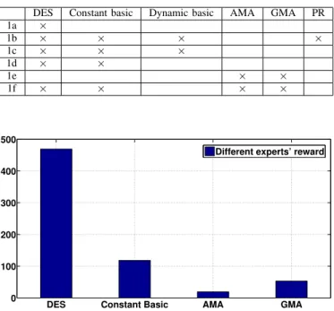
selected by the forecaster to build its prediction depend on the video content considered. For instance, the video content 1b selected the DES, Constant Basic, Dynamic basic and Polynomial Regression as the best experts over time, whereas the video content 1e selected AMA and GMA as the best experts. Table I justifies the fact that we need to use different experts. In addition, simulation results show that these best experts vary over time. Hence, a forecaster is needed to select the best experts at any given time.
TABLE I: Best experts for different contents.
DES Constant basic Dynamic basic AMA GMA PR
1a × 1b × × × × 1c × × × 1d × × 1e × × 1f × × × ×
DES Constant Basic AMA GMA
0 100 200 300 400 500
Different experts’ reward
Fig. 5: Rewards obtained by different experts. Figure 5 depicts the rewards obtained by the experts considered for the video content 1f. An expert is rewarded each time its cumulated loss belongs to the K > 1 smallest ones. We observe that DES is considered as a best expert 465 times, whereas AMA is selected only 23 times. This illustrates the importance of the forecaster’s role.
We now evaluate the best experts with regard to three ob-jectives we want to minimize simultaneously. These obob-jectives
are 1) the cumulated loss, 2) the maximum instantaneous loss and 3) the inverse of the reward. We consider two video contents: 1a for Figure 6 and 1b for Figure 7. For each content, we depict the accuracy of three experts, each expert minimizing an objective.
Fig. 6: The objectives minimized for content 1a.
Fig. 7: The objectives minimized for content 1b.
As observed in Figures 6 and 7, no expert simultaneously minimizes the three objectives. However, in Figure 6, we notice that the DES expert with parameters ow = 14 and α = 0.99 maximizes the reward and minimizes the cumulated loss. The expert minimizing the maximum instantaneous loss has a poor reward. It is rarely selected as a best expert. In Figure 7, we obtain similar conclusions but with different experts. The expert maximizing the reward and minimizing the cumulated loss is DES with the parameter α = 0.99. The Geometrical Moving Average adjusted expert is the one minimizing the maximum instantaneous loss.
IV. CONCLUSION
Machine learning techniques can be used in CDNs to predict the popularity of video contents. Each expert uses its own prediction method to build its prediction. In this paper, we evaluated the performances of a wide range of experts using various prediction methods (e.g. exponential smoothing, basic, adjustment with different corrections, polynomial regression, Savitzky Golay filtering). We used real traces of video content solicitations in YouTube CDN. Simulation results show that, on the one hand, the best experts (i.e. those minimizing the cumulated loss) depend on the profile of the video content considered, and on the other hand, the best experts vary over time. This is why we introduced a decision maker, called a forecaster, that builds its own prediction from the predictions given by the best experts. By comparing two types of fore-casters we concluded that the KBE forecaster outperforms the BE forecaster. In a further work, we will use the content popularity predictions to decide the contents that will be cached in the nodes near the end user. A certain percentage of a cache size will be reserved for the most popular contents. The remaining storage capacity will be shared among the solicited contents depending on their predicted popularity. Such a caching technique will be compared with classical techniques in terms of hit ratio.
REFERENCES
[1] G. Szabo and B. A. Huberman, Predicting the popularity of online content, Communications of the ACM, vol. 53, no. 8, pp. 8088, 2010. [2] H. Pinto, J. M. Almeida, and M. A. Goncalves, Using early view patterns
to predict the popularity of youtube videos, in Proceedings of the sixth ACM international conference on Web search and data mining. ACM, 2013, pp. 365374.
[3] M. Ahmed, S. Spagna, F. Huici, and S. Niccolini, A peek into the future: Predicting the evolution of popularity in user generated content, in Proceedings of the sixth ACM international conference on Web search and data mining. ACM, 2013, pp. 607616.
[4] G. Gursun, M. Crovella, and I. Matta, Describing and forecasting video access patterns, in INFOCOM, 2011 Proceedings IEEE. IEEE, 2011, pp. 1620.
[5] X. Gu, and H. Wang Online Anomaly Prediction for Robust Cluster Systems, ICDE 2009, Shanghai, China.
[6] Y. Wen, R. Wolski, and C. Krintz Online Prediction of Battery Lifetime for Embedded and Mobile Devices, PACS 2005
[7] F. Salfner, M.Lenk, and M. Malek A Survey of Online Failure Prediction Methods, CSUR 2010
[8] J. Kang, S. Seo , and J.W. Hong Personalized Battery Lifetime Prediction
for Mobile Devices based on Usage Patterns, JCSE 2011
[9] D. Marinca, P. Minet, and N. Ben Hassine An Efficient Learning Tech-nique to Predict Link Quality in WSN, PIMRC 2014, Washington, USA. [10] N. Cesa-Bianchi and G. Lugosi, Prediction, learning, and games,
Cambridge University Press, 2006.
[11] R. Shumway, D. Stoffer, Time Series Analysis and Its Applications, Springer, 2013
[12] D. Tong, Z. Jia, X. Qin, C. Cao, C. Chang, An Optimal Savitzky-golay Filtering Based Vertical Handoff Algorithm in Heterogeneous Wireless Networks, Journal of Computers, November 2014.
[13] N. Ben Hassine, D. Marinca, P. Minet, D. Barth, Popularity Prediction in Content Delivery Networks, PIMRC 2015, Hong-Kong, China, September 2015.