Computational image analysis of subcellular dynamics in time-lapse fluorescence microscopy

Computational Image Analysis of Subcellular

Dynamics in Time-Lapse Fluorescence Microscopy

by

Austin V. Huang

B.S. Electrical Engineering and Computer Science University of California, Berkeley, 2002

Submitted to the Department of Electrical Engineering and Computer Science

in partial fulfillment of the requirements for the degree of Ba-chelor of Science in Computer Science and Engineering

at the

MASSACHUSETTS INSTITUTE OF TECHNOLOGY

September 2004

©

Author ... ...

Department of Electrical Engineering and Computer Science

14 /September2)1, 2004

Certified by ...

/omas Lozano#erez

Professor f Computer Science and Engineering Thesis Supervisor Certified by .... . ...

Paul Matsudaira

Pr9fess o~Biology, Professor of Bioengineering

Thezs-Supervisor Accepted by ...

Arthur C. Smith Chairman, Department Committee on Graduate Students

MASSACHUSETTS INST11JTE OF TECHNOLOGY

MITLibraries

DISCLAIMER OF QUALITY

Due to the condition of the original material, there are unavoidable flaws in this reproduction. We have made every effort possible to

provide you with the best copy available. If you are dissatisfied with this product and find it unusable, please contact Document Services as soon as possible.

Thank you.

The images contained in this document are of

the best quality available.

Archives copy contains grayscale images only. This is the

best copy available.

Computational Image Analysis of Subcellular Dynamics in

Time-Lapse Fluorescence Microscopy

by

Austin V. Huang

Submitted to the Department of Electrical Engineering and Computer Science on September 21, 2004, in partial fulfillment of the

requirements for the degree of

Bachelor of Science in Computer Science and Engineering

Abstract

The use of image segmentation and motion tracking algorithms was adapted for ana-lyzing time-lapse data of cells with fluorescently labeled protein. Performance metrics were devised and algorithm parameters were matched to hand-created ground-truth data. The performance of these algorithms in this domain was compared. Finally, the optimal algorithms were selected and used to acquire statistics on existing data, in order to reproduce previous studies on the cell cytoskeleton. New data was ac-quired to extend previous results and further test the algorithms on a different cell line, under both widefield and confocal microscope conditions.

Thesis Supervisor: Tomas Lozano-Perez

Title: Professor of Computer Science and Engineering Thesis Supervisor: Paul Matsudaira

0.1

Acknowledgments

First of all, I would like my mother and father as well as the rest of my family. In particular - my grandparents, for funding my undergraduate education.

I would also like to thank my labmates, who have been fine company throughout

this work. In particular, some data in this thesis was from previous work by James Evans, who also introduced me to the "world" of cell culture.

I would like to thank the following out-of-lab experts for helpful discussions: Chris

Stauffer, Eric Grimson, Polina Golland, B.K. Horn, and John Fisher. To this group,

I would like to extend my apologies if I have asked any naive questions.

Last but not least, I must thank my advisors, Tomas Lozano-Perez and Paul Matsudaira for their guidance and support.

Contents

1.4.1 Segmentation . . . . 1.4.2 Motion Analysis . . . .

1.5 Evaluation of Motion Analysis Methods. .

2 Experimental Methods and Image Preprocessing

2.1 Experimental Methods . . . . 2.1.1 M aterials . . . . 2.1.2 Cell Culture . . . .

2.1.3 Sample Preparation for Imaging . . . .

2.1.4 M icroscopy . . . . 2.2 Preprocessing . . . . 2.2.1 Preprocessing of Widefield Images . . . . . 2.2.2 Preprocessing of Confocal Images . . . . .

3 Segmentation

3.1 Approximating the Cell Boundary using Histogram approximation

3.2 Segmentation of Podosomes by Thresholding . . . .

5 9 . . . . 10 . . . . 11 . . . . 13 . . . . 14 . . . . 14 . . . . 15 . . . . 18 21 . . . 21 . . . 22 . . . 22 . . . 22 . . . 23 . . . 24 24 . . . 25 27 28 30

3.3 3.4 3.5 3.6

Segmentation of Podosomes by Dynamic Thresholding . Segmentation of Podosomes by Laplacians . . . . Segmentation of Podosomes by the Watershed Algorithm Microtubule Segmentation . . . .

31

. . . . 32 . . . . 33 . . . . 34 4 Tracking and Statististics Acquisition

4.1 Podosome Fission and Fusion . . . . 4.2 Nearest-Neighbor . . . . 4.3 Kalman Filter Tracking . . . . 4.4 Intensity-Based Tracking . . . . 4.5 Statistics Acquisition and Data Visualization .

37 . . . . 38 . . . . 39 . . . . 4 1 . . . . 43 . . . . 44

5 Parameter Optimization and Algorithm Evaluation 5.1 Segmentation Parameter Optimization . . . .

5.1.1 Segmentation Ground Truth . . . .

5.1.2 Segmentation Performance Metric . . . .

5.2 Tracking Parameter Optimization . . . . 5.3 Tracking Ground Truth and Tracking Performance Metric 6 Results and Discussion

6.1 Segmentation Performance . . . .

6.2 Tracking Performance . . . .

6.3 Validating Algorithms against Previous Observations . . .

6.4 Tracking Podosomes in 3Y1-SR cells . . . .

6.5 Microtubule Segmentation . . . . 47 48 49 49 51 51 53 53 . . . . . 54 57 . . . . . 60 . . . . . 63 7 Future Work

7.1 Recursive Segmentation and Tracking . . . .

7.2 Improved Data Representation . . . .

7.3 Limitations of Data Acquisition Throughput . . . .

65 65 65 66

Chapter 1

Background

Bioimaging studies use microscopy to study the spatial and temporal characteristics of cells under controlled experimental conditions. This research is important in the study of sub-cellular processes which involve spatial, temporal, and mechanical regulation of proteins. Cellular motility is an important example of such a process.

To facilitate these studies, computational analysis tools to quantify the motion in microscopy images are needed. The purpose of this thesis is to investigate the use and extension of motion estimation algorithms for this purpose.

An example of the utility of such an endeavor is Valloton's [1] work in Fluorescence speckle microscopy. That work applied image analysis algorithms to quantify dynamic trends in the assembly of actin and tubulin polymers during cell migration and mitosis. Their work found previously unchracterized trends, such as the modulation of actin flow near the leading edge and a bidirectional flow of tubulin during mitosis. Such trends may not have been detected without the aid of algorithms to sort through the quantity of information in image sequences.

Isolated work has been done previously in applying image analysis algorithms to microscopy. But often little is said, beyond a qualitative argument, of why algorithms were chosen and how the parameters of those algorithms were set. Here a unified review of the work that has been done is provided, and a framework of optimizing and selecting image algorithms is demonstrated. Finally, the results of those optimization and selection procedure is applied to a model experimental system to confirm that

lightsao/re epi-lJunfirtdion ok/ective~ s tple dhCCD ligt of dfori C usr

Figure 1-1: Schematic of a widefield microscope, from [2].

the results agree with previously reported trends and to extend those results.

1.1

Fluorescence Microscopy

The data presented here consists primarily of images acquired either through widefield fluorescence microscopy or confocal fluorescence microscopy.

A widefield fluorescence microscope (see figure 1-1) consists of a light source such

as a mercury lamp, which emits light that is filtered through an excitation filter, reflected off a dichroic mirror and focused onto the sample by an objective lens [3]. The fluorescent molecules in the sample absorb photons and are excited (i.e. the potential energy is increased) and emit photons at a lower frequency, a phenomenon referred to as Stokes shift. The emitted photons pass back through the objective lens, through the dichroic mirror, through an emission filter tuned to the emission frequency of the fluorescent molecules, and onto a detector.

A confocal microscope (see figure 1-2) operates identically to a widefield

micro-scope, with the exception of a pinhole in front of the detector, which only allows light from a single focal point to hit the detector. The excitation source is also a laser rather than a mercury lamp, to excite only a small region of the sample at a time.

-- - - ---- - -.--- ~

laser Source

ilhunination pinhole

dt'teclor

[

ob!jective

Iocil plne

sample

Figure 1-2: Schematic of a confocal microscope, from [2].

or a motorized piezo actuator underneath the objective. This automation allows the focal plane to mechanically section the sample while acquiring images at specified vertical distance intervals. The axes convention commonly used (followed here) is to refer to the two horizontal axes as the X and Y axes, while the vertical axis is the Z axis.

1.2

Experimental Limitations

As with any real-world source of data, microscopy images are noisy, partial descrip-tions of the underlying state of the specimen. Here we examine the limitadescrip-tions on how images describe the underlying state of the specimen and the tradeoffs that can be made in determining the signal quality of the images.

The resolution limit of light microscopy due to the wavelength of light is a limi-tation in precision due to the properties of light. Events occurring on a scale smaller than this limit (e.g. actin filament polymerization) cannot be resolved, although they may be detectable. A consequence of this is that any information at a higher fre-quency than that dictated by this resolution limit is noise, and thus images can be lowpass filtered at the frequency corresponding to the resolution limit without any loss of information. The resolution limit can be calculated as [3]:

.=*61A

D = 61 (1.1)

n(NA)

Where A is the emission wavelength, n is the refractive medium of the medium between the specimen and the objective, and NA is the numerical aperture of the

objective. These values are all known parameters of the microscope.

Another important experimental limitation is photobleaching. When a fluores-cent molecule is in its excited state, it may undergo a chemical reaction with other molecules in the local environment and become a stable molecule which is no longer excitable. The longer a population of fluorescent molecules is excited, the higher the probability for each individual molecule that it loses its excitability. Thus over time, the fraction of photobleached molecules increases, reducing the amount of signal. Yet, the specimen must be illumnated for a longer integration period if a better signal-to-noise is to be obtained, or if the experiment is to run for a longer period of time. Unphotobleached fluorescent molecules can be preserved for a longer experiment by acquiring images less frequently, but temporal aliasing will occur when the specimen changes at a timescale less than the temporal sampling rate.

Noise is also introduced by the detector. The standard detector used in most microscopes is a coupled charge device (CCD) camera. A CCD detector is a rectan-gular array of imaging elements which count the arrival of photons. At the end of an integration period of time of the camera, each imaging element emits a current proportional to the number of photons which arrived. The arrival of photons at the camera is governed by a Poisson random process [4]:

p( p~pT ) = (( pT )P) ex p( -pT)/p! (1.2)

Where p is the number of photons, p is the number of photons per second, and

T is the integration time. Thus this noise is Poisson and not additive Gaussian, as

many noise models assume.

Errors may also be introduced in the analysis stages, for example image segmenta-tion is usually imperfect. Thus each phase in the image analysis should be as robust

as possible to errors introduced in the previous phase.

1.3

Cellular Motility

The study of the biochemical and physical mechanisms of cell motility is an important active area of research. Movement involves hundreds of cytoskeletal proteins which interact with each other in a system that involves both chemical and mechanical inter-actions. This makes the study of cellular motility particularly suited for bioimaging techniques, since bioimaging offers information on the spatial and temporal charac-teristics of proteins in live cells.

An understanding of cellular motility is important to human health. For instance, scientists look to understand the mechanisms of cell movement in order to discover ways of stopping that movement in cancer cells and preventing them form metastasiz-ing (spreadmetastasiz-ing to other parts of the body). Another example are immune deficiency disorders such as Wiskott-Aldrich syndrome, in which cells of the immune system exhibit decreased motility, and thus are unable to reach sites of infection. In this case we would like to understand the mechanisms of cell motility in order learn how to rehabilitate the motile ability of those cells.

The typical framework for cell motility studies is to perturb a specific biological subsystem of the cell in a biochemical or mechanical fashion and observe the change in behavior. From the changes in behavior, one can deduce the function of the subsystem that was perturbed. In order to perform these studies in a high-throughput and rigorous manner, there must be quantitative measurements for changes in behavior.

A review by Maheshwarei [5] describes common statistics that can be calculated

on entire cell populations to quantify how cellular motility of entire cell populations is affected by various perturbations.

The same principle of perturbing a system and quantifying the change in behavior may also be applied on a smaller scale. Within individual cells, the temporal and spa-tial characteristics of proteins and organelles can be studied using molecular probes. Some examples of this type of study are [6], [7], [8], and [1].

At the subeellular level, cell motility involves the cell cytoskeleton. The cytoskele-ton [3] is a network of fibers in the cell which is formed and controlled by an interacting system of proteins. The structure of the cytoskeleton changes in order to provide the contractile and protrusive forces needed for cell movement.

Two critical proteins within the cytoskeleton are Actin and Tubulin. Both pro-teins are polarized propro-teins which can polymerize into long chains. Tubulin protein polymerizes to form a network of microtubules. Microtubules are the largest fibers in the cytoskeleton (24 nm in diameter) and are classically known for their role in cell division, but are now also hypothesized to transport signaling proteins throughout the cell to regulate the behavior of other cytoskeletal components [9] [7]. Actin is present throughout the cell, and performs many functions in the cytoskeleton. Actin can bundle into stress fibers, providing contractile force, and is also found in sites of adhesion at the cell membrane where the cell attaches to a surface.

In certain cell types, a specific type of adhesion known as a Podosomes, is thought to play a key role in cell motility (see figure 1-3). Podosomes occur primarily in cells that are motile and must move through tissue [10]. They are visible in fluorescence images where Actin or other podosome associated proteins are tagged. This thesis uses podosomes as a model system for studying the quantification of dynamics at a subcellular scale.

1.4

Applicability of Computer Vision Methods

The areas of computer vision most directly relevant to this work are reviewed in this section. This discussion is not meant as a comprehensive overview of computer vision. The focus here is on image/video interpretation techniques dealing with segmentation and motion analysis that can be applied in this domain.

1.4.1 Segmentation

Segmentation is the transformation of a raw image into a reduced representation specific to a problem [11]. It is a classic problem in computer vision, but still active

Key:

GeKOM ~ Pyk4? M1 TalW1 Fimbr.

P13K C 1 Vonuin WASp CDC42

F

TRENDS CaN B."gy

Figure 1-3: Model of a Podosome, from

[10].

researched since there is no general solution. Most applicable to the work here is the segmentation work that has been done on medical imaging. For example, vesicle extraction techniques [12] may be applicable to the segmentation of microtubules in cells.

1.4.2

Motion Analysis

This work is not the first to apply motion quantification techniques from computer vision to microscopy. Some motion estimation techniques have been previously at-tempted in time-lapse microscopy.

Object Tracking

Out of all image motion analysis techniques, the one that has been applied to mi-croscopy the most is point tracking. The data representation of the underlying state to be estimated is a set of points that represents the object or objects. These points must be associated between time points to form tracks. In practice, these points may correspond to points on the image, for example, cells, podosomes, vesicles, or other

objects. Alternatively, rather than one point representing each object of interest, there may be larger objects whose representation is a set of points.

Much work has been done in radar [13] [14] [15] and computer vision [11] fields on multiple point tracking. Yet some aspects of point tracking are still active areas of research [16]. One reason for the difficulty and the continuing work on such a simple problem is the task of predicting motion between time points to improve the correctness of data correspondence between time points. Another practical issue which makes the problem difficult is when there exists a varying number of points to be tracked, which presents difficulties in detecting new points, detecting the deletion of points, and reducing the constraints which can be imposed on the set of track solutions.

Early applications of point tracking techniques to bioimaging work was done in the 90s. Tracking was done on low density lipoprotein receptor molecules [17] and later on entire cells [18].

The use of adaptive filtering to aid tracking of objects in video microscopy was first applied by Ngoc [19]. In this work, the data representation of the objects was a correlation filter (otherwise known as "block matching") which was adaptively up-dated in each frame. The data presented in their paper was primarily of transmission images.

C. Quentin Davis et. al. point out in [20], there are similarities and equivalences

between this correlation filter approach to tracking and optical flow, thus Ngoc's methods could be thought of as a combination of object tracking and the motion field estimation techniques discussed in the next section.

Point tracking has also been a necessity in fluorescence speckle microscopy (FSM) studies due to the large number of points that must be tracked to extract useful infor-mation [1]. In FSM, the imaging experiment is designed such that fraction of tagged molecules is intentionally low [21]. This experimental design has several desirable implications, one of which is that only a fraction of the total protein is tagged so that tagged proteins are sparse enough to be spaced farther apart than the resolution limit due to light. Trafficking and turnover of individual proteins can be extracted

by examining the dynamics of individual dots.

This approach contrasts with traditional fluorescence staining techniques, in which the density of tagged protein is much higher than the resolution limit, so little in-formation can be obtained about the trajectory of individual proteins. On the other hand, traditional staining techniques can offer information about larger structures of protein aggregates and achieve a higher signal-to-noise than FSM.

The approach to tracking taken in previous FSM studies have been to optimize the structure of a graph representing object correspondence, subject to a set of heuristic constraints [1]. This is an operations research perspective to the problem of object tracking, and is different from the approaches investigated and evaluated in this work.

3D point tracking was used by Zoe Demou

[22].

track entire cells in a 3D matrix was implemented. Cell tracking tends to be simpler than tracking sub-cellular structures since the motion of the entire cells typically occurs on a slower time scale. A fluorescent stain of the nucleus allows for obtaining cell centroids with less ambiguity.

Motion Field Estimation

Motion field estimation is a classic computer vision problem. The motion field is the gradient field of velocity projections produced by the image of a moving object. In the context of microscopy, since the image data is either two-dimensional (by transmission or fluorescent methods) or a three-dimensional stack (using fluorescent imaging on a confocal microscope) rather than a 2D projection of a 3D scene, the motion field is the velocity field of the actual object. Unfortunately, typical assumptions made

by motion field estimation methods don't always hold. For example, the temporal

sampling rate can be low due to experimental constraints, which can cause movies to violate certain smoothness assumptions.

Early work in this area was the development of algorithms to calculate optical flow by Horn and Shunck [23]. Optical flow is the apparent motion of the brightness pattern [24]. In most cases, it corresponds, or is highly correlated with the motion field, though there are certain, well-known exceptions [24].

Some work has been done in applying motion field estimation techniques to light microscopy. Florence Germain et al [25] calculated optical flow constrained by a parametric motion model in order to describe cell deformation and migration in low-magnification light microscope images. This approach neatly encodes qualitative descriptions of image dynamics (rotation, stretching, translation, etc.) with a low dimensional set of parameters.

Saskia van Engeland [26] and Tammo Delhaas [27] used a hierarchical feature vector matching (HFVM) method to generate a similar motion field. Unlike the parametric motion model approach, this approach estimates values for each point of the motion field. Their work uses the motion field to describe the motion of fluores-cently labeled microtubules in a cell. The initial segmentation of the microtubules was accomplished manually. Unlike the object tracking methods in the previous sec-tion, the results showed motion quantification of pixels corresponding to microtubules rather than a higher-level data representation of the objects (microtubules) of inter-est. Although HFVM is presented as a new technique, it is basically a variation on the optical flow algorithm with a brightness constraint applied to a set of filtered versions of the images.

Dennis Freeman and C. Quentin Davis have used variations on optical flow algo-rithms on video microscopy images to make sub pixel motion displacement measure-ments [28]. They apply this method to analyzing the tectorial membrane and MEMS devices [29].

Motion field estimation is an alternative representation of the underlying state to be estimated. Motion field estimation techniques are outside the scope of this work, but we include this review for completeness.

1.5

Evaluation of Motion Analysis Methods

There are few papers published on the evaluation of multiple object tracking al-gorithms, perhaps because the performance is often problem specific. Constraints particular to an individual application are often leveraged in tracking algorithms.

Zheng [30] presents a review of the tracking algorithms in the radar literature. He describes three main categories of multiple target tracking performance measures: correlation statistics, track maintenance statistics, and kinematic statistics. Corre-lation statistics are based on intermediate results. It examines small-scale statistics, such as the probability of a correct association between two objects in two adjacent time points. In contrast, track maintenance statistics are global measures of how well a track is maintained over time. Finally, kinematic statistics are based on statistics extracted from the tracks.

Veenman [31] provides a ground truth data set that is often used in scoring mul-tiple object tracking performance in computer vision. The data consists peas in a rotating dish. Successful solutions to this usually rely on the constraint of a one-to-one correspondence of points in adjacent time points. Since objects in fluorescent microscopy images undergo fusion and fission, this performance measure is not ap-propriate for evaluation of the methods presented here.

Chapter 2

Experimental Methods and Image

Preprocessing

2.1

Experimental Methods

As stated in 1.3, podosomes were used as a model system to quantify subcellular dy-namics. Thus, cells needed to be maintained for experiments, and podosomes needed to be fluorescently tagged in preparation for imaging. The affect of microtubule-inhibiting cancer drugs on Podosomes was used as a test experiment to test the tracking algorithm.

Previous work suggests that there is a relationship between the system of micro-tubules and adhesion sites [7] [9], including podosomes [6]. Demecolcine and Pacli-taxol are anti-cancer drugs that inhibit the working of the microtubule system in the cell, thereby preventing cell division.

To study the affect of those drugs on podosomes, transformed fibroblast cells (3Y1-SR) were transfected so that the Actin protein in the cell would be marked with a green fluorescent protein marker and could be seen under a fluorescence microscope. Cells prepared as such were treated with the anti-cancer drugs and imaged.

Additional data was acquired from previously done work by Dr. James G. Evans, under similar experimental conditions on mouse macrophages, obtained on a Zeiss LM-510 confocal microscope. The specific sample preparation and image

preprocess-ing steps are detailed in his paper [6].

2.1.1

Materials

* RPMI Media

" Fetal Bovine Serum " Penicillin-Streptomycin

" T-25 flasks (Corning Life Sciences Item #430639). " 6 Well Plate (Corning Life Science Item #3506) " Polypropylene Tubes (Falcon Item #2063)

* Opti-MEM media

" Lipofectamine 2000 (Invitrogen Part #52887)

" Glass Bottom Dishes (Mattek Part #P35G-1.5-20-C)

2.1.2

Cell Culture

SR-3Y1 cell lines are mouse fibroblasts that have been transformed by Rous Sarcoma Virus. They were cultured in RPMI media with 10% Fetal Bovine Serum and 1% penicillin-streptomycin. Cells were cultivated are split every 4-5 days when they become approximately 70-80% confluent.

2.1.3

Sample Preparation for Imaging

The protocol for transfecting the cells with Actin GFP DNA was the following:

1. Day One: Plate cells onto a six well plate.

(a) For each well, 4pg of Actin GFP was diluted with 250puL Opti-MEM and incubated for 5 minutes at room temperature. After incubation, 10PL of Fugene 2000 transfection reagent diluted with 250pL Opti-MEM was added.

(b) The mixture of DNA and transfection reagent is incubated for 15 minutes

and then 500pL of the mixture is added to each well.

3. Day Three: Detach cells and plate onto Mattek glass-bottom dishes.

4. Day Four: Introduce drugs into Mattek dishes 20-30 minutes prior to imaging. The drug conditions used were an untreated cell, a cell treated with Demecol-cine, and a cell treated with Paclitaxol. 1 micromolar Demecolcine was added to destabilize microtubules, while 10 micromolar paclitaxol was added to stabi-lize microtubules. Drug concentrations are the same as those used on previous experiments on IC-21 macrophages as described in

[6].

2.1.4

Microscopy

For each dataset, a single cell was imaged which occupies the majority of the field of view at 100x magnification. One cell of each drug condition was imaged under a Perkin Elmer Ultraview Spinning disk confocal microscope and a Spectris Deltavision widefield microscope. The Spectris Deltavision widefield images were taken on a 100x objective, with 2x2 binning, and a pixel size was 129nm x 129nm.

For each dataset, a single cell was imaged which occupies the majority of the field of view at 100x magnification. One cell of each drug condition was imaged under a Spectris Deltavision widefield microscope. The Spectris Deltavision widefield images were taken on a 100x objective, with 2x2 binning, and a pixel size was 129nm x 129nm.

2.2

Preprocessing

Since podosomes in cells on glass are present only at the bottom of the cell, two-dimensional images are usually sufficient to analyze their dynamics. However, a 3D z-stack is still collected for each time point to compensate for z-drift. The image is initially preprocessed in order to extract a 2D series of images that corresponds t and compensate for photobleaching.

2.2.1

Preprocessing of Widefield Images

The microscope stage expands and contracts due to fluctuations in temperature, causing the sample to fluctuate in z over time. To compensate, a stack of z-slices was taken for each time point, which included out of focus slices as well as the focal plane. This ensured that, even if the sample drifted vertically over the course of the experiment, the correct focal plane was still captured, so long as the sample did not drift out of the boundaries of the z stack.

The correct focal plane is found using the a method recommended by Boddeke [4]. Theoretically, the in-focus plane will have the highest amount of signal energy at the maximum spatial frequency that can be imaged by the optics of the microscope.

A method of finding the focal plane would be to bandpass filter the image near the

cutoff frequency and select the z slice which has the maximum energy when passed through the filter.

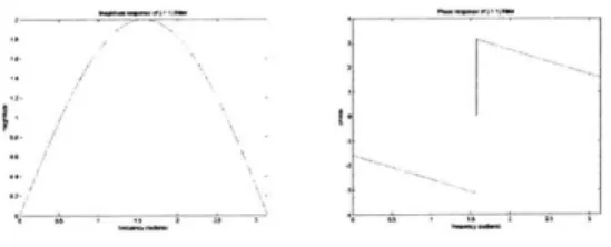
When the image is sampled close to the Nyquist frequency corresponding to the cutoff frequency of the microscope, the bandpass filter should be centered at the Nyquist frequency of 7r/2. A filter with an impulse response of [-11] is a 1-dimensional filter with this characteristic (see figure 2-1). A filter with such an impulse response is applied both horizontally and vertically to the image. As a 1-dimensional filter, it is fast, and the two orientations are sufficient to extract the energy characteristics of the z slice.

The signal strength of the image becomes weaker over time due to photobleaching. An ensemble of GFP exhibits an exponential intensity bleaching characteristic [32].

Figure 2-1: Frequency response characteristics of the autofocus filter.

Hence, an exponential curve was fitted to the average image intensity vs. time using a non-linear least squares curve fit. Only pixels in the cell (see 3.1 for how in-cell pixels were determined) were used to calculate the mean image intensity. The inverse of the fitted exponential function was used as the scaling factor to boost the image intensity, compensating for photobleaching. This method compensates for the decrease in image intensity, but the signal to noise still decreases with each exposure.

2.2.2

Preprocessing of Confocal Images

The same issues of bleach correction and z-drift correction were present in confocal data. Since out-of-focus light is not present in each slice of a z-stack, the focus-based criteria for selecting a slice is not appropriate. in this case. In the absence of out-of-focus light, the a mean-intensity profile curve over all the z slices could be used to

align the slices over time.

As seen in 2-2, the intensity profile in the data used here has a characteristic maximum that was used to align the slices.

The slices near the glass which correspond to the podosome data were picked out in the first time point and automatically selected in all subsequent time points using the alignment information provided by the intensity profiles. The slices were averaged for each time point, providing a single 2D projection of the podosomes over time.

Figure 2-2: Normalized mean-intensity profiles of confocal data over time. Blue indicates earlier time points, red indicates later time points.

Chapter 3

Segmentation

Segmentation is the transformation of a raw image into a reduced representation

[11].

In particular, the information from an image is initially reduced to a labeled image. The input to this segmentation process is the preprocessed image of a cell. The output is a segmentation "image" of the same dimensions as the input, but rather than intensity values, the numbers in each pixel correspond to the group label the

pixel belongs to (in this case, 0 = background, 1 = first podosome, 2 = 2nd podosome,

3 = 3rd podosome, etc.). Before tracking, the labeled image is further reduced to a set of coordinates, one per group labeling. Since the core of a Podosome is Actin-dense, the coordinate that represents each podosome is the pixel with maximal intensity in the original intensity image which is also a pixel labeled as belonging to the podosome. One issue is that while there is a correlation between image intensity and protein density, no calibration techniques exist to quantify the protein density from the image intensity. This makes the design criteria of the segmentation algorithm difficult. Even if one could quantitatively define a podosome as having a core of actin of a certain protein density, there is no existing method of translating such a definition into a classification rule on an image.

Here we discuss some segmentation methods employed to estimate a segmentation and in the next chapter the problem of selecting parameters for these algorithms will

be addressed.

3.1

Approximating the Cell Boundary using

His-togram approximation

Finding an approximation to the cell boundary is important for calibrating the inten-sities of the image using only the pixels within the cell boundary. Between different images, there are always varying amounts of blank space outside the boundaries of the cell. Intensity thresholds and other parameters specified only in terms of the statistics of intensities of the entire image would be skewed by the amount of blank space in the image. Consequently, determining the cell boundary improves calibration of the image intensities and is necessary to generalize optimal intensity-related parameters between different datasets.

There are trace amounts of actin throughout the cell as well as some autofluo-resence everywhere in the cell. Hence, there should be some signal throughout the majority of the cell body even though only actin should be tagged. This property can be exploited to extract a cell boundary from a protein-tagged image.

The image should contain a region of signal with noise (cell body), and a region of pure noise. This characteristic should be reflected in the brightness distribution function, [24] the histogram of intensities in an image.

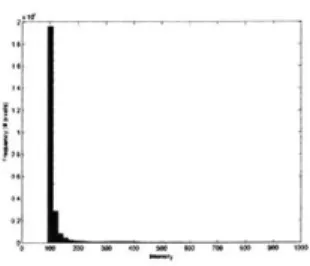
A histogram of intensities which is normalized to integrate to 1 is the discrete form

of a brightness distribution function. The histogram of intensities of the widefield images 3.1 show this characteristic of a densely populated peak of background noise and an extended flat region of signal+noise intensities corresponding to the region of the cell.

This signal+noise/noise segmentation characteristic is used in a thresholding scheme proposed by Ramesh

[33].

Figure 3-1: Example histogram of image intensities.

the average frequencies within the noise and signal intensity region, respectively. t is the free parameter to be optimized.

The algorithm proposes two criteria on which to optimise the model, minimization of the sum of square errors:

t = arg min EI[I - I] (3.1)

t

where E, denotes expectation with respect to intensity, I, p(I) denotes the proba-bility of an intensity, L denotes the maximal intensity. t, H1, and H2 correspond to the parameters of the approximation function f(I) described above. Another proposed objective function is to minimize the sum of the error variance:

t

-o

ft

2_{p(I) (3.2)}

t =arg min +

(

t EI=0 P(I) it P(I)

Ramesh derives a method of optimizing the function parameters by iterative ap-proximation. Their method was found to perform well for non-bimodal intensity his-tograms, which is the case with microscopy data. Of the two algorithms, minimum variance performed better, according to their work. From a qualitative standpoint, this was seen in the data acquired as well, and thus the minimum-variance criteria was used.

An alternative approach to determining the cell boundary is to use multiple fluo-rescence excitation/emission frequency channels. Appropriate stains are available to label the entire cell with a whole cell stain. Two sets of images could be captured, one

Figure 3-2: Computing the cell boundary. Blue and green denote background and foreground, respectively, as computed by Ramesh's minimum-variance threshold es-timator [33]. The white boundary is the convex hull, which is used as the boundary of the cell.

at the emission frequency of the stain for the cell boundary and one for the protein of interest, such actin. Drawbacks to this method are that the collection of two emission frequencies of data reduces the maximum temporal sampling rate by a half and that there is always some overlap in the excitation/emission spectra of the two dyes.

3.2

Segmentation of Podosomes by Thresholding

Podosomes consist of a dense, actin core. Thus, with actin tagged by GFP, one should theoretically be able to identify podosomes by thresholding, that is, marking all pixels as being above or below an intensity threshold.

The most basic image segmentation technique is to apply an intensity threshold to the image. For a comprehensive comparison of thresholding methods, see [34]. Pixels above the intensity threshold are labeled as 1, and pixels below the intensity threshold are labeled as 0, creating a bitmap of binary values, called a binary image. From the binary image, a segmented image where pixels corresponding to podosomes are given a value of the enumerated with one integer given for each different podosome is produced by labeling connected components in the image.

In order to generalize an optimal threshold between multiple datasets, the thresh-old values are specified in terms of the number of standard deviations from the mean intensity. The statistics for standard deviation and mean intensity are specified in terms of pixels within the cell.

Thresholding uses a single parameter - a threshold intensity value.

Figure 3-3: Thresholding-based segmentation on synthetic data.

0.51

2

Figure 3-4: 2D Fourier Transform of the operation of subtracting a local average from the image.

3.3

Segmentation of Podosomes by Dynamic

Thresh-olding

Dynamic thresholding augments thresholding by taking into account low-frequency variations in the background intensity [35]. For every pixel, the average pixel intensity within a local region is subtracted from the pixel's intensity before thresholding. This can be accomplished by creating a kernel of size NxN uniformly filled with the value 1/N 2. The kernel is convolved with the image to obtain an averaged image. The averaged image is subtracted from the original image to obtain a difference image and this difference image is thresholded. The operation of obtaining the difference image can be thought of as a linear operation with a 2D Fourier Transform shown in figure 3-4. Connected components are then labeled as in 3.2.

Dynamic thresholding has two parameters - the size of the averaging kernel and an intensity threshold for the difference image. The intensity threshold is specified in terms of standard deviations from the mean intensity of pixels within the cell.

3.4

Segmentation of Podosomes by Laplacians

Laplacians are commonly used to detect edges in images where intensity is chang-ing fastest [11]. Since podosomes correspond to intensity peaks in the image, they may be detected by the decreasing intensity contours which surround them. Thus boundary pixels in the derivative image are a local maximum and in the second derivative image are a zero-crossing.

The Laplacian is the sum of the partial second derivative images [11]:

(V2_{f)(, y) = + (33)}

Therefore object boundaries can be marked by zero-crossings in the Laplacian image.

The image is first convolved with a Gaussian filter to smooth the image to prevent discontinuities (otherwise derivative images will undefined at the discontinuity loca-tions) and to limit the impact of high frequency noise. The operations of smoothing and derivatives can be combined into a single, linear filter (see figure 3-6). Thus, the algorithm applied to segment structures using Laplacians was:

1. Obtain image of region boundaries by filtering the image with a

Laplacian-of-Gaussian Filter (figure 3-5, first image).

2. Symmetrically copy the edge image so that objects on image boundaries will be closed. (figure 3-5, second image)

3. Fill in all closed regions in the image, producing a binary image. mask this

binary image with a low threshold to remove low-intensity noise. (figure 3-5, third image)

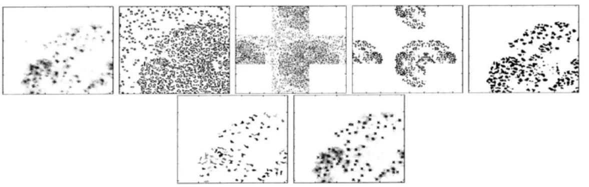
4. Crop the central portion of the binary image. Each pixel in the binary image is median filtered over a 3 time-point window to smooth segmentation changes over time. (figure 3-5, fourth image)

1 71

- 1.

Figure 3-5: Segmentation by Laplacians.

Figure 3-6: Impulse response of a Laplacian of Gaussian filter and it's associatied 2D Fourier Transform.

5. Each 8-way connected set of pixels is marked as a distinct region. (figure 3-5,

sixth image)

6. Centroid coordinates for each marked region are marked as the pixel with peak

intensity in the original image that lies within the marked set of pixels. (figure

3-5, seventh image).

The parameters of the Laplacian method of segmentation are the low-intensity background threshold and the minimum area of an object.

3.5

Segmentation of Podosomes by the Watershed

Algorithm

Watershed algorithms have been used to segment clustered objects, such as cells [36]. The watershed algorithm first finds the local maxima of intensities. The maxima

are used as seeds to dilate into regions until they come into contact with each other. Regions are not merged once they have dilated to come into contact with each other. Rather, a boundary is placed when two regions intersect and neither region grows in the direction of the other region as other regions are dilated. When the entire image is filled with regions, this process is stopped. The original algorithm was developed

by Vincent and Soille [37] and was inspired by the behavior of flooding water, hence

its name.

In a sense, the watershed algorithm is the opposite of the edge-detection based Laplacian algorithm. Instead of finding structure boundaries and filling them in, it begins with centers and fills the structures outwards.

In order to smooth the region boundaries, a 2D Gaussian filter is applied to the image prior to the application of the watershed algorithm.

The parameters of watershed-based segmentation are standard deviation of the Gaussian filter used to smooth the image and the low-intensity background threshold.

3.6

Microtubule Segmentation

Although microtubule segmentation and tracking is not the primary focus of this work, some work was done on segmenting microtubule data.

The image characteristics of microtubules when the cell is not dividing is that they are filamentous structures emanating from a microtubule organization center (MTOC). The MTOC is a complex of proteins underneath the nucleus that organizes microtubules in cells.

1. Specify a small, representative horizontal and vertical microtubule within the

image as a match filter template. Normalise the intensities of the filter to be zero-mean.

2. Filter the image with the horizontal and vertical match filters and threshold the result, obtaining two binary images corresponding to regions in the image corresponding to microtubules.

Figure 3-7: Microtubules in an SV-3Y1 cell. The nucleus has been stained blue and the microtubules have been stained red. There is a higher density of microtubules at the microtubule-organizing center at the center of the cell.

Chapter 4

Tracking and Statististics

Acquisition

Tracking is the inference of object state from time-series data [11]. An object is some physical component of the sample that is to be analyzed - in this case, podosomes. The data is a time-series set of images. The input to the tracking algorithms are the results of a segmentation algorithm applied to the set of images in the experiment. The outputs of the tracking algorithm are the state values corresponding to each object at every time point, describing the dynamics of the objects. One useful value for an object state is the centroid of the object. But others, such as volume, or parametric shape descriptors may be used as well.

In this domain of tracking structures and objects imaged by microscopy, there are several additional complexities that are introduced. Firstly, there are often many objects of interest. Multiple objects must be tracked and the correct correspondences between time points must be made. Secondly, the objects are very dynamic and not always conserved. Structures such as podosomes often undergo fusion and fission processes. Allowing a wider variety of object dynamics causes the tracking solutions to be less constrained.

An important distinction is that, although podosomes may appear as moving points with a life span, and are abstracted as such in the segmentation, they are in actuality an aggregate of proteins. When podosomes appear to move, it is not a

Figure 4-1: Podosome fission.

cohesive object that is moving (as is the case for vesicles), but rather the appearance of motion due to the occurrence of polarized polymerization whereby the protein polymerizes at one end of the podosome and depolymerizes in the other.

For this work, the representation of each object is the coordinate of maximal intensity and the input to the tracks is a set of coordinates over time. However, the same principles could be applied to a more complex object representation, such as a parameterized shape or the first several moments of an object.

4.1

Podosome Fission and Fusion

The formation of podosomes is an active area of research [10]. The signaling mecha-nisms by which podosomes are assembled and disassembled are actively researched. Past work has shown that podosome assembly and disassembly do not occur in ran-dom locations, but in close proximity to existing podosomes [6] [38]. One method of podosome formation is the fission of an existing podosome. A podosome is constantly surrounded by a lower-intensity pool of actin. Actin drawn from this pool becomes more dense and creates a new podosome nearby.

An understanding of podosome assembly and disassembly is a primary motivation for quantifying the dynamics of podosomes, and thus a data representation of the dynamics must include object fusion and fission.

In 4.1, we see two podosomes undergoing fission. Actin from the "cloud" associ-ated an older podosome extends in a direction and condenses into a new podosome. From this image, we see the newly created podosome is formed far enough away from the older podosome so that after the fission event, a clear determination can be made as to which was the "parent" and which was the "child."

was a intensity-based method determination and one was a distance-gating method. The distance-gating method assumes that, within a small gating distance, po-dosome centroids are sufficiently close so that the low-intensity clouds which sur-round them must exchange actin and thus they are undergoing fusion/fission. The Nearest-neighbor and Kalman Filter algorithms use this method of detecting fusion and fission. The nearest-neighbor specifies a gate as a Euclidean distance, while the Kalman Filter specifies the gate in terms of the Mahalanobis distance. An interest-ing question is whether the more dynamic probabilistic representation will provide a genuine improvement in the detection of fission and fusion events.

The intensity-based method explicitly examines the low-intensity distribution of actin to find connectivity between the low-intensity clouds surrounding the po-dosomes. The intensity-based tracking algorithm uses this method of detection fission and fusion.

4.2

Nearest-Neighbor

Nearest neighbor is the simplest method of associating objects between time points. It relies on the assumption that the time points are sufficiently well-sampled in time that the most probable position of an object in the following time point is the position of the object nearest to the object in the current time point. There are two tunable parameters in nearest-neighbor tracking. A fission distance gate and an object asso-ciation distance gate. Tracking proceeds in two phases.

First, an object association graph is created. The object association graph is an undirected graph with each vertex representing a centroid at a particular time point and edges corresponding to object associations between adjacent time points.

A vertex exists for every centroid of every time point. In the absence of fusion and

fission, every fully connected subgraph in the association graph encodes the dynamics of a particular object.

Because fusion and fission of objects is allowed, a vertex may have zero, one or multiple edges connecting it to objects in adjacent time points. Certain statistics, such

40, 35, 30, 25, S20, F 10, 5f 250 0 200~' 2 0 0 200 250 150 <- 00 Ws Y 100 50

Figure 4-2: An Object Association Graph.

as the frequency of object fusion/fission can be extracted from the object association graph alone.

Once the object association graph has been created, sets of edges are grouped into tracks. Tracks are initiated at the first time point, when a new object was detected, or when a fission occurs.

At each time point, each centroid is checked, if it is associated with a centroid from a previous time point, and there was no fission event at the centroid in the previous time point, it is grouped into the same track as the previous time point.

If there is a fission in the association graph where a single centroid is associated

with two objects, the parent podosome continues to be tracked as the edge corre-sponding to the nearest association, while the creation of new daughter podosomes correspond to object associations that are farther than the nearest association. A new track is initiated for each daughter podosome

If a centroid has no associations from the previous time point, it initiates a new

track.

The end of a track occurs if a centroid has no associations in the association graph to objects of the following time point.

4.3

Kalman Filter Tracking

Kalman Filter tracking is a standard tracking algorithm used in computer vision and radar. It is a recursive algorithm in which a dynamic model is used to predict the motion of a tracked object. The prediction at each time point is used to determine the object in the next time point which corresponds to the tracked object at in the current time point. The new information about the object at the next time point is used to update the state of the dynamic model. A state is kept per object and the association graph and the track maintenance is done in a single pass rather than divided into two separate passes.

In this application of the Kalman filter, its potential usefulness is to use a dynamic model to predict object motion in order to achieve better object association. Objects in biology are often known to have some persistence characteristic, if an object moves in a certain direction, it is often most likely to continue in the same direction. This characteristic is known to be true of cells [5], and qualitatively, it has was observed in our data of subcellular structures as well. Using this persistence characteristic could theoretically overcome reduce ambiguities in object correspondence between time points.

A linear dynamic model was used, described by the transformation matrix D:

D=( (At) (4.1)

Each detected distinct object had a single Kalman filter that was updated over time. The state vector for each object was:

x

X = Y(4.2)

dx dt di

state space to be estimated for each object.

A matrix

Q stores the process noise covariance while a matrix R stores the

mea-surement error covariance. These matrices describe the uncertainty in the process model and the measurement model, respectively. There are methods to measure these, however, in practice, they can also be thought of as tunable parameters to be optimized, which is the approach taken in this work.

The Kalman Filter can be described as a recursive process that iterates for each time point. First, a prediction is made based on the current state of the object and the dynamic model. Based on the prediction, a centroid from the following time point is associated with the track. The new associated centroid provides a new measurement used to update the state of the object. In addition to the state, an error covariance variable is maintained to quantify the accuracy of the predictions. Based on the error covariance, a weighting factor, called the Kalman gain, is computed which weighs the prediction against the measured centroid in estimating the object location.

1. Predict the state of the object and its predicted error covariance:

.k= DXk- 1 (4.3)

P- = DPk1 DT +

Q

2. Based on the prediction, associate the nearest object within a maximal distance gate. Also associate "split" objects as any object within a "fission" distance gate.

3. Using the associated object as the centroid measurement for the next time point,

calculate the Kalman gain. Use the Kalman gain to correct the object state and error covariance:

Kk = P yH T (HPJHT + R) (4.5) Xk = xx~ + Kk (zk - H.p-) (4.6)

Pk= (I - KkH) P- (4.7)

4. Repeat the procedure from the prediction step using updated state parameter values.

As with nearest-neighbor tracking, centroids not associated with a previous time point and fission events initiate new tracks. As before, at each fission event, the parent continued to be tracked as the nearest of all correspondences, while each of the farther correspondences initiates a new "daughter" track. The only difference is that the fission and association gate is specified not in terms of the Euclidean distance, but in terms of the Mahalanobis distance, D, in terms of the error covariance matrix

P, the predicted centroid location x-, and the coordinates of the object being tested

Zk for a correspondence:

D = (x- - Zk)P- (xk - Zk)' (4.8)

The description here was of this particular use of the Kalman filter. For a more detailed introductory treatment of the Kalman filter, see [39] or [11]. For a more rigorous treatment of the Kalman filter, see Roger E. Kalman's original paper [40].

4.4

Intensity-Based Tracking

Another approach to detecting fusion and fission events is by examining the local image data near the podosome.

In particular an histogram-equalized image is pre-calculated for each of the images in the time series. Histogram equalization is a standard contrast-enhancing technique in which the intensity levels are adjusted so that there are an equal number of pixels

Figure 4-3: Histogram equalization applied to an image of an SR cell. An inverted gray colormap was used in both images. The first image is the raw image, the second image is contrast-enhanced by histogram equalization.

for every intensity level in the dynamic range. The intensity histogram is computed using only in-cell pixels, where the in-cells pixels are determined by the method in section 3.1.

Recall that two podosomes are undergoing fission or fusion if they are near enough and connected by a low intensity actin cloud, as shown in figure 4.1. This property is used to determine object correspondences - a threshold to segment actin clouds is specified in terms of the normalized histogram-equalized image intensities. Assuming that distribution of fluorescence intensity within the cell remains relatively constant, this makes the segmentation of actin clouds less susceptible to noise and changes in cell shape and size.

A correspondence is made between two objects in two different time points of the

association graph so long as they fall within an association gate and they lie within actin clouds which contain pixels that overlap.

These rules generate an object association graph, from which, tracks are combined from sets of graph edges using the same algorithm as 4.2

4.5

Statistics Acquisition and Data Visualization

Statistics are acquired from the segmentation and tracking analysis to mine the images for correlations between observable events.

compare the results with previous studies. Many more can be extracted directly from the association graph, tracks, cell boundary, and segmentation information that was generated by these methods.

The fraction of podosomes undergoing fusion and fission were extracted and plot-ted over time using the association graph. A time-average of this was calculaplot-ted for each dataset.

The lifetime of podosomes was calculated from the set of tracks produced by the tracking algorithms. A histogram of lifetimes was produced and an average podosome lifetime was calculated.

Podosome size is measured from the labeled segmentation images. The distances inter-podosome distances were measured using the podosome coordinates by finding the distance to the nearest podosome for each podosome. Podosome density for each time point was found by dividing the number of podosomes by the size of the cell. These three statistics were acquired for future use, and were not analyzed for any biological significance in this work.

The results of the tracking algorithm was also visualized to check for possible tracking errors. A 3D kymograph view similar to the visualization method used in