HAL Id: hal-00450854
https://hal.archives-ouvertes.fr/hal-00450854v2
Submitted on 27 Aug 2010
HAL is a multi-disciplinary open access
archive for the deposit and dissemination of
sci-entific research documents, whether they are
pub-lished or not. The documents may come from
teaching and research institutions in France or
abroad, or from public or private research centers.
L’archive ouverte pluridisciplinaire HAL, est
destinée au dépôt et à la diffusion de documents
scientifiques de niveau recherche, publiés ou non,
émanant des établissements d’enseignement et de
recherche français ou étrangers, des laboratoires
publics ou privés.
Discrete Carleman estimates for elliptic operators in
arbitrary dimension and applications
Franck Boyer, Florence Hubert, Jérôme Le Rousseau
To cite this version:
Franck Boyer, Florence Hubert, Jérôme Le Rousseau. Discrete Carleman estimates for elliptic
oper-ators in arbitrary dimension and applications. SIAM Journal on Control and Optimization, Society
for Industrial and Applied Mathematics, 2010, 48 (8), pp. 5357-5397. �10.1137/100784278�.
�hal-00450854v2�
IN ARBITRARY DIMENSION AND APPLICATIONS
FRANCK BOYER† §, FLORENCE HUBERT‡ §, AND J´ER ˆOME LE ROUSSEAU¶
Abstract. In arbitrary dimension, we consider the semi-discrete elliptic operator −∂2
t + AM,
where AM is a finite difference approximation of the operator −∇x(Γ(x)∇x). For this operator
we derive a global Carleman estimate, in which the usual large parameter is connected to the dis-cretization step-size. We address disdis-cretizations on some families of smoothly varying meshes. We present consequences of this estimate such as a partial spectral inequality of the form of that proven by G. Lebeau and L. Robbiano for AM and a null controllability result for the parabolic operator
∂t+ AM, for the lower part of the spectrum of AM. With the control function that we construct
(whose norm is uniformly bounded) we prove that the L2-norm of the final state converges to zero
exponentially, as the step-size of the discretization goes to zero. A relaxed observability estimate is then deduced.
Key words. Elliptic operator – discrete and semi-discrete Carleman estimates – spectral in-equality – control – parabolic equations.
AMS subject classifications. 35K05 - 65M06 - 93B05 - 93B07 - 93B40
1. Introduction and settings. Let d ≥ 2, L1, . . . , Ldbe positive real numbers,
and Ω = Q
1≤i≤d
[0, Li]. We set x = (x1, . . . , xd) ∈ Ω. With ω b Ω we consider the
following parabolic problem in (0, T ) × Ω, with T > 0,
∂ty − ∇x· (Γ∇xy) = 1ωv in (0, T ) × Ω, y|∂Ω= 0, and y|t=0= y0, (1.1)
where the diagonal diffusion tensor Γ(x) = Diag(γ1(x), . . . , γd(x)) with γi(x) > 0
satisfies
reg(Γ)def= sup
x∈Ω i=1,...,d ³ γi(x) + 1 γi(x) + |∇xγi(x)| ´ < +∞. (1.2)
The null-controllability problem consists in finding v ∈ L2((0, T ) × Ω) such that y(T ) = 0. This problem was solved in the 90’s by G. Lebeau and L. Robbiano [LR95]
and A. Fursikov and O. Yu. Imanuvilov [FI96].
Let us consider the elliptic operator on Ω given by
A = −∇x· (Γ∇x) = −
P
1≤i≤d
∂xi(γi∂xi)
with homogeneous Dirichlet boundary conditions on ∂Ω. We shall introduce a finite-difference approximation of the operator A. For a mesh M that we shall describe below, associated with a discretization step h, the discrete operator will be denoted
Date: August 27, 2010
∗The three authors were partially supported by l’Agence Nationale de la Recherche under grant
ANR-07-JCJC-0139-01.
†Universit´e Paul C´ezanne ([email protected]). ‡Universit´e de Provence ([email protected]).
§Laboratoire d’Analyse Topologie Probabilit´es (LATP), CNRS UMR 6632, Universit´es
d’Aix-Marseille, 39 rue F. Joliot-Curie, 13453 Marseille cedex 13, France.
¶Universit´e d’Orl´eans, Laboratoire Math´ematiques et Applications, Physique Math´ematique
d’Orl´eans (MAPMO), CNRS UMR 6628, F´ed´eration Denis Poisson, CNRS FR 2964, Bˆatiment de Math´ematiques, B.P. 6759, 45067 Orl´eans cedex 2 ([email protected]).
by AM. It will act on a finite dimensional space CM, of dimension |M|, and will be
selfadjoint for a suitable inner product in CM. Our main result is a Carleman-type
estimate for the “extended” semi-discrete elliptic operator, −∂2
t + AM. Here, the
additional variable t is not directly connected to the time variable in the parabolic problem above. In the discrete setting, such a result was obtained in [BHL09a] in the one-dimensional case. Here, we extend this result to any space dimension. Note that we also prove a Carleman estimate for AMitself. For Carleman estimates in the
continuous case we refer to [H¨or63, Zui83, H¨or85, LR95, FI96, LR97, LL09]. Note that an earlier attempt at deriving discrete Carleman estimates can be found in [KS91]. The result presented in [KS91] cannot be used here as the condition imposed by these authors on the discretization step size, in connection to the large Carleman parameter, is too strong for the applications we have in mind to the problem of uniform controllability properties for semi-discrete parabolic problems.
We now describe an important consequence of the Carleman estimate we prove, which was the main motivation of this work. We denote by φM a set of discrete
orthonormal eigenfunctions, φj ∈ CM, 1 ≤ j ≤ |M|, of the operator AM, and by
µM = {µ
j, 1 ≤ j ≤ |M|} the set of the associated eigenvalues sorted in a
non-decreasing sequence. The following (partial) spectral inequality is then a corollary of the semi-discrete Carleman estimate we prove:
P µk∈µM µk≤µ |αk|2= R Ω ¯ ¯ ¯ P µk∈µM µk≤µ αkφk ¯ ¯ ¯2≤ CeC√µR ω ¯ ¯ ¯ P µk∈µM µk≤µ αkφk ¯ ¯ ¯2, ∀(αk)1≤k≤|M|⊂ C, (1.3) for µh2 ≤ C
S with CS and h sufficiently small (integrals of discrete functions are
introduced below). This type of spectral inequality goes back to the work of G. Lebeau and L. Robbiano [LR95] (see also [LZ98a, JL99]). As opposed to the continuous case this inequality is not valid for the whole spectrum. The condition µh2≤ C
S with CS
small, states that it is only valid for a constant lower portion of the spectrum. This condition cannot be relaxed. The optimal value of CS is not known at this point and
certainly depends, at least, on the geometry of ω.
The spectral inequality (1.3) then implies the null-controllability of system (1.1) for the lower part of the spectrum µ ≤ CS/h2, i.e., for any initial condition y0∈ CM,
there exists a control v in L2((0, T ) × Ω) (the semi-discrete functional spaces we
shall use will be made precise below) with kvkL2((0,T )×Ω) ≤ C|y0|L2(Ω) such that
(y(T ), φk) = 0 if µkh2 ≤ CS. Moreover, the remainder satisfies |y(T )|L2(Ω) ≤
e−C/h2
|y0|L2(Ω). We thus obtain an exponential convergence as h goes to 0. Accurate
statements of the results we have just described are given in Section 1.2.
The form of the relaxed observability estimate that follows from this controllabil-ity result has been the inspiration for the study of Carleman estimates for semi-discrete parabolic operators [BHL10]. The spectral inequality (1.3) is also at the heart of the work carried out by the authors on the numerical analysis of the fully-discretized parabolic control problem in [BHL09b].
In two dimensions, for finite differences, there is a counterexample to the null and approximate controllabilities for uniform grids on a square domain for distributed or boundary controls due to O. Kavian (see [Zua06]). It exploits an explicit eigenfunction of AMin two dimensions that is solely localized on the diagonal of the square domain.
This eigenfunction is associated with an eigenvalue in the higher part of the spectrum. Our result may thus seem rather optimal in dimension greater that two.
In dimension one, there is a null controllability result due to A. Lopez and E. Zuazua [LZ98b] for the entire spectrum in the case of a constant diffusion co-efficient and for a constant step size finite-difference discretization. In dimension one, our method based on the proof of discrete Lebeau-Robbiano spectral inequality can-not achieve such a result. In fact, one can can-notice that (1.3) cancan-not hold for the full spectrum. In dimension one, the generalization of the result of [LZ98b] to a non constant coefficient and non uniform meshes remains an open problem.
We now present the precise settings we shall work with. For 1 ≤ i ≤ d, i ∈ N, we set Ωi= Q 1≤j≤d j6=i [0, Lj]. For T > 0 we introduce Q = (0, T ) × Ω, Qi = (0, T ) × Ωi, 1 ≤ i ≤ d.
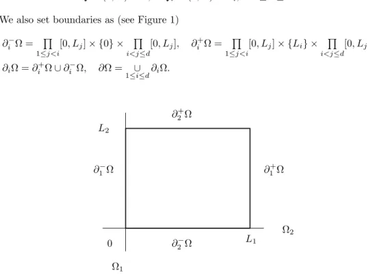
We also set boundaries as (see Figure 1)
∂− i Ω = Q 1≤j<i [0, Lj] × {0} × Q i<j≤d [0, Lj], ∂+i Ω = Q 1≤j<i [0, Lj] × {Li} × Q i<j≤d [0, Lj], ∂iΩ = ∂i+Ω ∪ ∂i−Ω, ∂Ω =1≤i≤d∪ ∂iΩ. 0 Ω1 ∂1+Ω Ω2 L1 L2 ∂1−Ω ∂2+Ω ∂2−Ω
Fig. 1. Notation for the boundaries
1.1. Discrete settings. Here, we precisely define the type of mesh and dis-cretization we shall use. The notation we introduce is technical, and yet will allow us to use a formalism as close as possible to the continuous case, in particular for norms and integrations. Then most of the computations we carry out can be read in a very
intuitive manner, which will ease the reading of the article. Most of the discrete
for-malism will then be hidden in the subsequent sections. The notation below is however necessary for a complete and precise reading of the proofs.
We shall use the notation Ja, bK = [a, b] ∩ N.
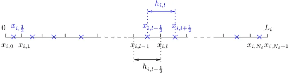
1.1.1. Primal mesh. For i ∈ J1, dK and Ni ∈ N∗, let
xi,l 0 xi,0 xi,1 xi,1 2 xi,l−1 hi,l−1 2 xi,l−1 2 xi,l+12 hi,l Li xi,Nixi,Ni+1
Fig. 2. Discretization in the ith direction.
We introduce the following set of indices,
N :=©k = (k1, . . . , kd); ki∈ J1, NiK, i ∈ J1, dK
ª
.
For k = (k1, . . . , kd) ∈ N we set xk = (x1,k1, . . . , xd,kd) ∈ Ω. We refer to this
discretization as to the primal mesh M :=©xk; k ∈ N
ª
, with |M| := Q
i∈J1,dK
Ni.
For i ∈ J1, dK and l ∈ J0, NiK we set
hi,l+1
2 = xi,l+1− xi,l, xi,l+12 = (xi,l+1+ xi,l)/2,
and
hi= max l∈J0,NiK
hi,l+1
2, i ∈ J1, dK, h = maxi∈J1,dKhi.
For i ∈ J1, dK and l ∈ J1, NiK, we set
hi,l= xi,l+1
2 − xi,l−12 = (hi,l+12 + hi,l−12)/2.
See Figure 2, where the introduced notation is illustrated.
1.1.2. Boundary of the primal mesh. To introduce boundary conditions in the ith direction and related trace operators (see Section 1.1.5) we set ∂iN = ∂i−N ∪
∂+ i N with ∂− i N = © k = (k1, . . . , kd); kj ∈ J1, NjK, j ∈ J1, dK, j 6= i, ki= 0 ª , ∂i+N =©k = (k1, . . . , kd); kj ∈ J1, NjK, j ∈ J1, dK, j 6= i, ki= Ni+ 1 ª , and ∂N = ∪ i∈J1,dK∂iN, ∂M = © xk; k ∈ ∂N ª , ∂± i M = © xk; k ∈ ∂i±N ª . Notice that ∂±
i M is nothing but the set of points of the primal mesh which are located
on the boundary ∂i±Ω.
1.1.3. Dual meshes. We will need to operate discrete derivatives on functions defined on the primal mesh (see Section 1.1.6). It is easily seen that these derivatives are naturally associated to another set of meshes, called dual meshes. In fact there will be two kinds of such meshes: the ones associated to first order discrete derivation
and the ones associated to second order discrete derivation. Let us define precisely these new meshes.
For i ∈ J1, dK, we introduce a second type of sets of indices Ni:=nk = (k1, . . . , kd); kj∈ J1, NjK j ∈ J1, dK, j 6= i, and ki= l + 1 2, l ∈ J0, NiK o .
For j ∈ J1, dK, j 6= i, we also set ∂jN
i = ∂− j N i ∪ ∂+ jN i with ∂− j N i =nk = (k1, . . . , kd); ki0 ∈ J1, Ni0K, i0∈ J1, dK, i06= i, i06= j, ki= l +1 2, l ∈ J0, NiK, and kj= 0 o , ∂+ j N i =nk = (k1, . . . , kd); ki0 ∈ J1, Ni0K, i0∈ J1, dK, i06= i, i06= j, ki= l +1 2, l ∈ J0, NiK, and kj= Nj+ 1 o , and ∂Ni= ∪j∈J1,dK j6=i ∂jN i . We moreover introduce ∂iN i = ∂− i N i ∪ ∂+ i N i with ∂− i N i =nk = (k1, . . . , kd); kj∈ J1, NjK, j ∈ J1, dK, j 6= i, ki= 1 2 o , ∂+ i N i =nk = (k1, . . . , kd); kj∈ J1, NjK, j ∈ J1, dK, j 6= i, ki= Ni+1 2 o . Remark that ∂iN i ⊂ Ni whereas ∂jN i 6⊂ Ni for j 6= i.
For i, j ∈ J1, dK, i 6= j, we introduce a third type of sets of indices Nij := n k = (k1, . . . , kd); ki0 ∈ J1, Ni0K, i0∈ J1, dK, i06= i, i06= j and ki= l1+1 2, l1∈ J0, NiK, kj= l2+ 1 2, l2∈ J0, NjK, o .
For l ∈ J1, dK, l 6= i, l 6= j, we also set ∂lN
ij = ∂l−Nij∪ ∂l+Nij with ∂− l N ij =nk = (k1, . . . , kd); ki0 ∈ J1, Ni0K, i0 ∈ J1, dK, i0 6= i, i06= j, i06= l, ki= l1+ 1 2, l1∈ J0, NiK, kj = l2+ 1 2, l2∈ J0, NjK, and kl= 0 o , ∂+l Nij = n k = (k1, . . . , kd); ki0 ∈ J1, Ni0K, i0 ∈ J1, dK, i0 6= i, i0 6= j, i0 6= l, ki= l1+1 2, l1∈ J0, NiK, kj = l2+ 1 2, l2∈ J0, NjK, and kl= Nl+ 1 o , and ∂Nij = ∪l∈J1,dK l6=i,l6=j∂lN ij . Moreover we set ∂iN ij = ∂− i N ij ∪ ∂+ i N ij with ∂−i Nij = n k = (k1, . . . , kd); ki0 ∈ J1, Ni0K, i0 ∈ J1, dK, i0 6= i, i0 6= j, ki= 1 2, kj= l + 1 2, l ∈ J0, NjK o , ∂+ i N ij =nk = (k1, . . . , kd); ki0 ∈ J1, Ni0K, i0∈ J1, dK, i0 6= i, i0 6= j, ki= Ni+1 2, kj= l + 1 2, l ∈ J0, NjK o .
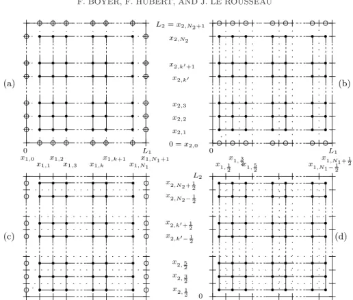
x1,1 x1,2 x1,3 x1,k x1,k+1 x1,N1 (a) (c) (b) x1, 1 2 x1, 3 2x1, 5 2 x1,N1−12 x 1,N1+12 L1 0 (d) x2,1 x2,2 x2,3 x2,k0 x2,k0+1 x2,N2 L2= x2,N2+1 0 = x2,0 x1,0 x1,N1+1 0 L1 x2, 3 2 x2, 5 2 x2, 1 2 x2,k0− 1 2 x2,k0+ 1 2 x 2,N2−12 x 2,N2+12 0 L2
Fig. 3. Primal mesh and dual meshes in the two-dimensional case. The mesh points are marked
by black discs. Available boundary mesh points are marked with white discs. (a) M and ∂M; (b)
M1and ∂M1; (c) M2 and ∂M2; (d) M12.
For k = (k1, . . . , kd) ∈ N
i
or ∂Ni(resp. Nijor ∂Nij) we also set xk= (x1,k1, . . . , xd,kd),
which gives the following dual meshes Mi:=©xk; k ∈ N iª , ∂Mi:=©xk; k ∈ ∂N iª , ∂j±Mi:=©xk; k ∈ ∂j±N iª , ¡ resp. Mij :=©xk; k ∈ N ijª , ∂Mij :=©xk; k ∈ ∂N ijª , ∂± l M ij :=©xk; k ∈ ∂l±N ijª¢ .
The geometry of the different meshes we have introduced is illustrated in Figure 2 in the two dimensional case.
In the present article, we shall only consider some families of regular non uniform meshes, that will be precisely defined in Section 1.1.8. Note that the extension of our results to more general mesh families does not seem to be straightforward.
1.1.4. Discrete functions. We denote by CM (resp. CMi or CMij) the sets of
discrete functions defined on M (resp. Mior Mij) respectively. If u ∈ CM(resp. CMi
or CMij), we denote by u
k its value corresponding to xk for k ∈ N (resp. k ∈ N
i or k ∈ Nij). For u ∈ CMwe define uM= P k∈N 1bkuk ∈ L ∞(Ω), with b k= Q i∈J1,dK [xi,ki−12, xi,ki+12], k ∈ N. (1.4)
Since no confusion is possible, by abuse of notation we shall often write u in place of uM. For u ∈ CM we define RR Ω u :=RR Ω uM(x) dx = P k∈N ¯ ¯bk ¯ ¯ uk, where ¯ ¯bk ¯ ¯ = Q i∈J1,dK hi,ki, k ∈ N.
For some u ∈ CM, we shall need to associate boundary values
u∂M=©u
k; k ∈ ∂N
ª
,
i.e., the values of u at the point xk∈ ∂M. The set of such extended discrete functions
is denoted by CM∪∂M. Homogeneous Dirichlet boundary conditions then consist in
the choice uk = 0 for k ∈ ∂N, in short u∂M= 0 or even u|∂Ω= 0 by abuse of notation
(see also Section 1.1.5 below).
Similarly, for u ∈ CMi (resp. CMij) we shall associate the following boundary
values u∂Mi=©u k; k ∈ ∂N iª ¡ resp. u∂Mij =©u k; k ∈ ∂N ijª¢ .
The set of such extended discrete functions is denoted by CMi∪∂Mi(resp. CMij∪∂Mij).
For u ∈ CMi (resp. CMij) we define
uMi= P k∈Ni 1bi kuk∈ L ∞(Ω) with bi k = Q l∈J1,dK [xl,kl−1 2, xl,kl+12], k ∈ N i , ³ resp.uMij = P k∈Nij 1bij kuk∈ L ∞(Ω) with bij k = Q l∈J1,dK [xl,kl−12, xl,kl+12], k ∈ N ij´ .
As above, for u ∈ CMi (resp. CMij), we define
RR Ω u :=RR Ω uMi(x) dx = P k∈Ni ¯ ¯bi k ¯ ¯ uk, where ¯ ¯bi k ¯ ¯ = Q l∈J1,dK hl,kl, k ∈ N i , ³ resp.RR Ω u :=RR Ω uMij(x) dx = P k∈Nij ¯ ¯bij k ¯ ¯ uk, where ¯ ¯bij k ¯ ¯ = Q l∈J1,dK hl,kl, k ∈ N ij´ .
Remark 1.1. Above, the definitions of bk, b
i
k, and b
ij
k look similar. They are
however different as each time the multi-index k = (k1, . . . , kd) is chosen in a different
set: N, Ni and Nij respectively.
With u(t) in CM(resp. CMi or CMij) for all t ∈ (0, T ), we shall writeRRR
Qu dt =
RT
0
RR
Ωu(t) dt. In particular we define the following L2 inner product on CM (resp.
CMi or CMij) (u, v)L2(Ω)= RR Ω uv∗=RR Ω uM(x)(vM(x))∗dx, (1.5) ³ resp. (u, v)L2(Ω)= RR Ω uv∗=RR Ω uMi(x)(vMi(x))∗dx, or (u, v)L2(Ω)= RR Ω uv∗=RR Ω uMij(x)(vMij(x))∗dx´.
The associated norms will be denoted by |u|L2(Ω). For semi-discrete function u(t),
t ∈ (0, T ), as above we shall also use the following L2 norm: ku(t)k2 L2(Q)= T R 0 RR Ω |u(t)|2dt.
1.1.5. Traces. Let i ∈ J1, dK. For u ∈ CM∪∂M (resp. CMj∪∂Mj, j 6= i), its trace
on ∂+i Ω, corresponds to k ∈ ∂i+N (resp. ∂i+Nj), i.e., ki = Ni+ 1 in our
discretiza-tion and will be denoted by u|ki=Ni+1 or simply uNi+1. Similarly its trace on ∂
− i Ω,
corresponds to k ∈ ∂−
i N (resp. ∂i−N
j
), i.e., ki = 0 and will be denoted by u|ki=0 or
simply u0. The latter notation will be used if no confusion is possible, if the context
indicates that the trace is taken on ∂− i Ω.
By abuse of notation, we shall also use ∂iΩ, i ∈ J1, dK, to denote the boundaries
of Ω in the discrete setting. For homogeneous Dirichlet boundary condition we shall write
v|∂iΩ= 0 ⇔ v|ki=0= v|ki=Ni+1= 0.
For v ∈ CMi∪∂Mi (resp. CMij∪∂Mij, j 6= i), its trace on ∂+
i Ω, corresponds to k ∈ ∂+ i N i (resp. ∂+ i N ij
), i.e., ki = Ni+12 in our discretization and will be denoted
by v|ki=Ni+1
2 or simply vNi+12. Similarly its trace on ∂
−
i Ω, corresponds to k ∈ ∂i−N
i
(resp. ∂−i Nij), i.e., ki = 12 and will be denoted by v|ki=12 or simply v12. The latter
notation will be used if no confusion is possible, if the context indicates that the trace is taken on ∂i−Ω.
For such functions u ∈ CM∪∂M (resp. CMj∪∂Mj, j 6= i) we can then define surface
integrals of the type R ∂+ iΩ u|∂+ iΩ= R Ωi u|ki=Ni+1= P k∈∂+i N (resp.k∈∂+i Nj ) ¯ ¯∂ibk ¯ ¯ uk, where¯¯∂ibk ¯ ¯ = Q l∈J1,dK l6=i hl,kl, k ∈ ∂ + i N (resp. ∂+i N j ), and for v ∈ CMi∪∂Mi (resp. CMij∪∂Mij, j 6= i)
R ∂+ iΩ v|∂+ iΩ= R Ωi v|ki=Ni+12 = P k∈∂+i Ni (resp.k∈∂+i Nij ) ¯ ¯∂ib i k ¯ ¯ vk, where¯¯∂ib i k ¯ ¯ = Q l∈J1,dK l6=i hl,kl, k ∈ ∂ + i N i (resp. ∂i+Nij). Observe that if k ∈ ∂+ i N (resp. ∂i+N j ) and k0∈ ∂+ i N i (resp. ∂+ i N ij ) with kl= k0l for l 6= i then¯¯∂ibk ¯ ¯ =¯¯∂ib i k0 ¯ ¯. We thus have R ∂+ iΩ v|∂+ iΩ= R Ωi v|ki=Ni+12 = R Ωi (τi−v)|ki=Ni+1= R ∂+ iΩ (τi−v)|∂+ iΩ where τ− i v ∈ CM∪∂ − i M (resp. CMj∪∂ −
i Mj) with the translation operator τi− defined in
Section 1.1.6. It is then natural to define the following integrals R Ωi uNi+1vNi+12 = R Ωi u|ki=Ni+1v|ki=Ni+12 = R Ωi (u τ− i v)|ki=Ni+1= R ∂+ iΩ u(τ− i v)|∂+ iΩ.
Such trace integrals will appear when applying discrete integrations by parts in the following sections.
Similar definitions and considerations can be made for integrals over ∂− i Ω.
For u ∈ CM∪∂M (resp. CMj∪∂Mj, j 6= i) we can then introduce the following L2
norm for the trace on ∂iΩ:
|u|2L2(∂ iΩ)= |u|∂iΩ| 2 L2(∂ iΩ)= R Ωi ¯ ¯u|ki=Ni+1 ¯ ¯2 +R Ωi ¯ ¯u|ki=0 ¯ ¯2 .
For v ∈ CMi∪∂Mi (resp. CMij∪∂Mij, j 6= i) we can then introduce the following L2
norm for the trace on ∂iΩ:
|v|2 L2(∂iΩ)= |v|∂iΩ| 2 L2(∂iΩ)= R Ωi ¯ ¯u|ki=Ni+1 2 ¯ ¯2 +R Ωi ¯ ¯u|ki=1 2 ¯ ¯2 .
1.1.6. Difference operators. Let i, j ∈ J1, dK, j 6= i. We define the following translations for indices:
τi±: Ni (resp. Nij) → N ∪ ∂i±N (resp. Nj∪ ∂i±Nj), k 7→ τ± i k, with (τ± i k)l= ( kl if l 6= i, kl±12 if l = i.
Translations operators mapping CM∪∂M→ CMi and CMj∪∂Mj → CMij are then given
by
(τi±u)k= u(τ±
i k), k ∈ N i
(resp. Nij).
A difference operator Di and an averaging operator Ai are then given by
(Diu)k= (hi,ki) −1((τ+ i u)k− (τi−u)k), k ∈ N i (resp. Nij), (Aiu)k= ˜uik= 1 2((τ + i u)k+ (τi−u)k), k ∈ N i (resp. Nij). Both map CM∪∂M→ CMi and CMj∪∂Mj → CMij.
We also define the following translations for indices:
τi±: N (resp. Nj) → Ni(resp. Nij), k 7→ τi±k, with (τ± i k)l= ( kl if l 6= i, kl±12 if l = i.
Translations operators mapping CMi→ CM and CMij → CMj are then given by
(τi±v)k = v(τ±
i k), k ∈ N (resp. N j
).
A difference operator Di and an averaging operator Ai are then given by
(Div)k= (hi,ki) −1((τ+ i v)k− (τi−v)k), k ∈ N (resp. N j ), (Aiv)k = vik= 1 2((τ + i v)k+ (τi−v)k), k ∈ N (resp. N j ). Both map CMi → CMand CMij → CMj.
1.1.7. Sampling of continuous functions. A continuous function f defined on Ω can be sampled on the primal mesh fM= {f (x
k); k ∈ N}, which we identify to
fM= P
k∈N
1bkfk, fk= f (xk), k ∈ N,
with bk as defined in (1.4). We also set
f∂M= {f (x
k); k ∈ ∂N}, fM∪∂M= {f (xk); k ∈ N ∪ ∂N}.
The function f can also be sampled on the dual meshes, e.g. Mi, fMi= {f (x
k); k ∈ Ni} which we identify to fMi= P k∈Ni 1bi kfk, fk= f (xk), k ∈ N i
with similar definitions for f∂Mi, fMi∪∂Mi and sampling on the meshes Mij, Mij ∪
∂Mij.
In the sequel, we shall use the symbol f for both the continuous function and its sampling on the primal or dual meshes. In fact, from the context, one will be able to deduce the appropriate sampling. For example, with u defined on the primal mesh, M, in the following expression, Di(γDiu), it is clear that the function γ is sampled
on the dual mesh Mi as Diu is defined on this mesh and the operator Di acts on
functions defined on this mesh.
To evaluate the action of multiple iterations of discrete operators, e.g. Di, Di, Ai, Ai
on a continuous function we may require the function to be defined in a neighborhood of Ω. This will be the case here of the diffusion coefficients in the elliptic operator and the Carleman weight function we shall introduce. For a function f defined on a neighborhood of Ω we set τi±f (x) := f ³ x ±hi 2ei ´ , ei= (δi1, . . . , δid), Dif := (hi)−1(τi+− τi−)f, Aif = ˆf i =1 2(τ + i + τi−)f.
For a function f continuously defined in a neighborhood of Ω, the discrete function
Dif is in fact Dif sampled on the dual mesh, M
i
, and Dif is Dif sampled on the
primal mesh, M. We shall use similar meanings for averaging symbols, ˜f , f , and
for more general combinations: for instance, if i 6= j, gDjf
i , DiDjf i , DiDjf i will be respectively the functions dDjf
i sampled on Mij, \DiDjf i sampled on M, and \DiDjf i sampled on Mj
1.1.8. Regular families of non-uniform meshes. In this paper, we address non uniform meshes that are obtained as the smooth image of an uniform grid.
More precisely, let Ω? = (0, 1) and let ϑ
i : R 7→ R, i ∈ J1, dK be increasing maps such that ϑi∈ C∞, ϑi(Ω?) = [0, Li], inf Ω?ϑ 0 i> 0. (1.6) Let h?
i = Ni1+1 and M0 be the following uniform primal mesh on [0, 1]
d M0= {x0k= (x01,k1, . . . , x 0 d,kd) = (k1h ? 1, . . . , kdh?d), k ∈ N},
and M0
i
, i ∈ J1, dK the associated dual meshes. We define a non uniform mesh on Ω
M = {xk, k ∈ N}, with xk= (ϑ1(x01,k1), . . . , ϑd(x 0 d,kd)) (1.7) We set h? = sup
i∈J1,dKh?i. Once the functions ϑi, i ∈ J1, dK, are fixed we assume
that for some C > 0 we have
Ch?≤ h?i ≤ h?, i ∈ J1, dK.
For the mesh M, this in turn implies, for some C0 > 0, for all i ∈ J1, dK,
C0h ≤ hi,l≤ h, l ∈ J1, NiK, C0h ≤ hi,l+1
2 ≤ h, l ∈ J0, NiK.
In particular,
C0h ≤ h
i≤ h, i ∈ J1, dK. (1.8)
We define the following quantities in order to measure the regularity of the meshes under study reg(ϑi) = max µ sup Ω? ϑ 0 i, sup Ω? (ϑ 0 i)−1, sup Ω? |ϑ 00 i| ¶ , reg(ϑ) = Qd i=1reg(ϑi).
Note that reg(ϑi) ≥ 1 for any i ∈ J1, dK.
We shall call uniform meshes, the regular meshes that are obtained with the following linear choice: ϑi(x) = Lix.
1.1.9. Additional notation. We shall denote by z∗ the complex conjugate of
z ∈ C. In the sequel, C will denote a generic constant independent of h, whose value
may change from line to line. As usual, we shall denote by O(1) a bounded function. We shall denote by Oµ(1) a function that depends on a parameter µ and is bounded
once µ is fixed. The notation Cµ will denote a constant whose value depends on the
parameter µ.
We say that α is a multi-index if α = (α1, . . . , αn) ∈ Nn. For α ∈ Nn and ξ ∈ Rn
we write |α| = α1+ · · · + αn, ∂α= ∂xα11· · · ∂ αn xn, ξ α= ξα1 1 · · · ξnαn.
1.2. Statement of the main results. With the notation we have introduced, a consistent finite-difference approximation of Au with homogeneous boundary con-ditions is
AMu = − P
i∈J1,dK
for u ∈ CM∪∂M satisfying u
|∂Ω = u∂M = 0. Recall that, in each term, γi is the
sampling of the given continuous diffusion coefficient γion the dual mesh M
i
, so that for any u ∈ CM∪∂Mwe have
(AMu) k= − P i∈J1,dK γi ³ xτ+ i k ´ ¡(τ+ i)2u ¢ k−uk h i,ki+12 − γi ³ xτ− i k ´u k− ¡ (τ− i )2u ¢ k h i,ki−12 hi,ki , k ∈ N.
Note however that other consistent choices of discretization of γi on the dual meshes
are possible, such as the averaging on the dual mesh Mi of the sampling of γi on the
primal mesh. Our results also holds for such discrete operators.
Remark 1.2. Finite differences are not well adapted to address anisotropic
el-liptic operators. Here, we only treat the case of a diagonal anisotropic operator, i.e. an anisotropy associated with the principal axes. Note however that the treatment we make of non uniform meshes naturally leads to such diagonal anisotropic operators by a change of variables, even starting from an isotropic diffusion coefficient.
We choose a function ψ that satisfies the following properties.
Assumption 1.3. Let ˜Ω be a smooth open and connected bounded neighborhood
of Ω in Rd and set ˜Q = (0, T ) × ˜Ω. The function ψ is in Cp( ˜Q, R), with p sufficiently
large, and satisfies, for some c > 0, |∇ψ| ≥ c and ψ > 0 in ˜Q,
∂niψ(t, x) < 0 in (0, T ) × V∂iΩ, ∂
2
iψ(t, x) ≥ 0 in (0, T ) × V∂iΩ,
∂tψ ≥ c on {0} × (Ω \ ω), ψ = Cst and ∂tψ ≤ −c on {T } × Ω,
where V∂iΩis a sufficiently small neighborhood of ∂iΩ in ˜Ω, in which the outward unit
normal ni to Ω is extended from ∂iΩ. The construction of such a weight function is
described in Section A. We then set ϕ = eλψ.
To state the Carleman estimate for the semi-discrete operator −∂2
t + AM, we
introduce the following discrete gradient operator
g
= (D1, . . . , Dd)t.Theorem 1.4. Let ϑi, i ∈ J1, dK satisfy (1.6) and ψ be a weight function satisfying
(1.3) for the observation domain ω. For the parameter λ ≥ 1 sufficiently large, there
exist C, s0≥ 1, h0> 0, ε0> 0, depending on ω, T , (ϑi)i∈J1,dK and reg(Γ), such that
for any mesh M obtained from (ϑi)i∈J1,dK by (1.7), we have
s3kesϕuk2L2(Q)+ skesϕ∂tuk2L2(Q)+ skesϕ
guk
2L2(Q)+ s|esϕ(0,.)∂tu(0, .)|2L2(Ω)+ se2sϕ(T )|∂tu(T , .)|2L2(Ω)+ s3e2sϕ(T )|u(T , .)|2L2(Ω) ≤ C ³ kesϕ(−∂t2+ AM)ukL22(Q)+ se2sϕ(T )|gu(T , .)|2L2(Ω) + s|esϕ(0,.)∂tu(0, .)|2L2(ω) ´ , (1.9) for all s ≥ s0, 0 < h ≤ h0 and sh ≤ ε0, and u ∈ C2([0, T ], CM∪∂M), satisfying u|{0}×Ω= 0, u|(0,T )×∂Ω= 0.
Denoting by φM a set of discrete L2 orthonormal eigenfunctions, φ
j ∈ CM, 1 ≤
j ≤ |M|, of the operator AM with homogeneous Dirichlet boundary conditions, and
by µM the set of the associated eigenvalues sorted in a non-decreasing sequence, µ
j,
Theorem 1.5 (Partial discrete Lebeau-Robbiano inequality). Let ϑ satisfying (1.6). There exist C > 0, ε1> 0 and h0 such that, for any mesh M obtained from ϑ by (1.7) such that h ≤ h0, for all 0 < µ ≤ ε1/h2, we have
P µk∈µM µk≤µ |αk|2= R Ω ¯ ¯ ¯ P µk∈µM µk≤µ αkφk ¯ ¯ ¯2≤ CeC√µR ω ¯ ¯ ¯ P µk∈µM µk≤µ αkφk ¯ ¯ ¯2, ∀(αk)1≤k≤|M|⊂ C.
The proof is given in [BHL09a, Section 6] following the approach introduced in [Le 07].
We introduce the following finite dimensional spaces
Ej = Span{φk; 1 ≤ µk≤ 22j} ⊂ CM, j ∈ N,
and denote by ΠEj the L
2-orthogonal projection onto E
j. The controllability result
we can deduce from the above results is the following.
Theorem 1.6. Let T > 0 and ϑ satisfying (1.6). There exist h0 > 0, CT > 0
and C1, C2, C3 > 0 such that for all meshes M defined by (1.7), with 0 < h ≤ h0, and all initial data y0∈ CM, there exists a semi-discrete control function v such that the solution to
∂ty −
P
i∈J1,dK
Di(γiDiy) = 1ωv, y∂M= 0, y|t=0= y0. (1.10) satisfies ΠEjMy(T ) = 0, for jM= max{j; 22j ≤ C1/h2}, with kvkL2(Q)≤ CT|y0|L2(Ω)
and furthermore |y(T )|L2(Ω)≤ C2e−C3/h 2
|y0|L2(Ω).
For a proof see [BHL09a, Section 7].
Finally, in the spirit of the work of [LT06] the controllability result we have obtained yields the following relaxed observability estimate
Corollary 1.7. There exist CT > 0 and C > 0 depending on Ω, ω, T , and ϑ,
such that the semi-discrete solution q in C∞([0, T ], CM) to
−∂tq + AMq = 0 in (0, T ) × Ω, q = 0 on (0, T ) × ∂Ω, q(T ) = qF ∈ CM,
in the case h ≤ h0, satisfies |q(0)|L2(Ω)≤ CT ³RT 0 R ω |q(t)|2 dt´ 1 2 + Ce−C/h2 |qF|L2(Ω).
As mentioned above, these results can also be used for the analysis of the space/time discretized parabolic control problem [BHL09b].
1.3. Outline. In Section 2 we have gathered preliminary discrete calculus re-sults. Many of the proofs of these results can be found in [BHL09a]. Additional proofs have been placed in Appendix B to ease the reading. Section 3 is devoted to the proof of the semi-discrete elliptic Carleman estimate for uniform meshes. Again, to ease the reading, a large number of proofs of intermediate estimates have been placed in Appendix C. This result is then extended to non-uniform meshes in Sec-tion 4. For completeness, in Appendix D we give the counterpart of the Carleman estimate of Theorem 1.4 in the case of a fully-discrete elliptic operator. This result will be used in [BHL10] for the treatment of semi-discrete parabolic operators.
2. Some preliminary discrete calculus results. Here, to prepare for Sec-tion 3, we only consider uniform meshes, i.e., constant-step discretizaSec-tions in each direction, i.e., hi,j+1
2 = hi=
Li
Ni+1, j ∈ J0, NiK, i ∈ J1, dK.
This section aims to provide calculus rules for discrete operators such as Di, Di
and also to provide estimates for the successive applications of such operators on the weight functions.
2.1. Discrete calculus formulae. We present calculus results for the finite-difference operators that were defined in the introductory section. Proofs are similar to that given in the one-dimension case in [BHL09a].
Lemma 2.1. Let the functions f1and f2be continuously defined in a neighborhood of Ω. For i ∈ J1, dK, we have Di(f1f2) = Di(f1) ˆf i 2+ ˆf i 1Di(f2).
Note that the immediate translation of the proposition to discrete functions f1, f2∈
CM(resp. CMj, j 6= i), and g
1, g2∈ CMi (resp. CMij, j 6= i) is Di(f1f2) = Di(f1) ˜f i 2+ ˜f i 1Di(f2), Di(g1g2) = Di(g1) gi2+ gi1Di(g2).
Lemma 2.2. Let the functions f1and f2be continuously defined in a neighborhood of Ω. For i ∈ J1, dK, we have d f1f2 i = ˆfi1fˆ i 2+ h2 i 4 Di(f1)Di(f2).
Note that the immediate translation of the proposition to discrete functions f1, f2∈
CM(resp. CMj, j 6= i), and g
1, g2∈ CMi (resp. CMij, j 6= i) g f1f2 i = ˜fi1f˜ i 2+ h2 i 4 Di(f1)Di(f2), g1g2 i= gi 1gi2+ h2 i 4 Di(g1)Di(g2).
Some of the following properties can be extended in such a manner to discrete functions. We shall not always write it explicitly.
Averaging a function twice gives the following formula.
Lemma 2.3. Let the function f be continuously defined in a neighborhood of Ω.
For i ∈ J1, dK we have A2if :=fbˆ ii = f +h 2 i 4 DiDif.
The following proposition covers discrete integrations by parts and related for-mulae.
Proposition 2.4. Let f ∈ CM∪∂M and g ∈ CMi. For i ∈ J1, dK we have
RR Ω f (Dig) = − RR Ω (Dif )g + R Ωi (fNi+1gNi+12 − f0g12), RR Ω f gi=RR Ω ˜ fig −hi 2 R Ωi (fNi+1gNi+12 + f0g12).
Lemma 2.5. Let i ∈ J1, dK and v ∈ CM∪∂M (resp. CMj∪∂Mj for j 6= i) be such that v|∂iΩ= 0. Then RR Ωv = RR Ω˜v i.
Lemma 2.6. Let f be a smooth function defined in a neighborhood of Ω. For
i ∈ J1, dK we have τ± i f = f ± hi 2 1 R 0 ∂if (. ± σhi/2) dσ, A`if = f + C`h2i 1 R −1 (1 − |σ|) ∂2 if (. + l`σhi) dσ, D` if = ∂i`f + C`0h2i 1 R −1 (1 − |σ|)`+1∂`+2 i f (. + l`σhi) dσ, ` = 1, 2, l1= 1 2, l2= 1, with hi = hiei. For i, j ∈ J1, dK, i 6= j, we have DiDjf = ∂ij2f + C00 |h+ij|4 hihj 1 R −1 (1 − |σ|)3f(4)(. + σh+ij/2; η+, . . . , η+) dσ + C000|h + ij|4 hihj 1 R −1 (1 − |σ|)3f(4)(x + σh− ij/2; η−, . . . , η−) dσ, with h±ij = hiei± hjej and η± =|h1± ij| (h±ij). Note that |h+ij|4 hihj = O(h 2) by (1.8), for i, j ∈ J1, dK, j 6= i. Proof. This series of results follow from Taylor formulae,
f (x + η) =n−1P j=0 1 j!f (j)(x; η, . . . , η) +R1 0 (1 − σ)n−1 (n − 1)! f (n)(x + ση; η, . . . , η) dσ, at order n = 1, n = 2, n = 3 or n = 4.
2.2. Calculus results related to the weight functions. We now present some technical lemmata related to discrete operations performed on the Carleman weight function that is of the form esϕwith ϕ = eλψ, ψ ∈ Cp, with p sufficiently large.
For concision, we set r = esϕ and ρ = r−1. The positive parameters s and h will be
large and small respectively and we are particularly interested in the dependence on
s, h and λ in the following basic estimates.
We assume s ≥ 1 and λ ≥ 1. We shall use multi-indices of the form α = (αt, αx)
with αt∈ N and αx∈ Nd.
Lemma 2.7. Let α and β be multi-indices. We have
∂β(r∂αρ) =|α||β|(−sϕ)|α|λ|α+β|(∇ψ)α+β (2.1)
+ |α||β|(sϕ)|α|λ|α+β|−1O(1) + s|α|−1|α|(|α| − 1)O
λ(1) = Oλ(s|α|).
Let σ ∈ [−1, 1] and i ∈ J1, dK. We have ∂β(r(x)(∂αρ)(x + σh
i)) = Oλ(s|α|(1 + (sh)|β|)) eOλ(sh). (2.2)
Provided sh ≤ K we have ∂β(r(x)(∂αρ)(x+σh
i)) = Oλ,K(s|α|). The same expressions
hold with r and ρ interchanged and with s changed into −s.
With Leibniz formula we have the following estimate. Corollary 2.8. Let α, β and δ be multi-indices. We have
∂δ(r2(∂αρ)∂βρ) =|α + β||δ|(−sϕ)|α+β|λ|α+β+δ|(∇ψ)α+β+δ + |δ||α + β|(sϕ)|α+β|λ|α+β+δ|−1O(1)
+ s|α+β|−1(|α|(|α| − 1) + |β|(|β| − 1))O
λ(1) = Oλ(s|α+β|).
The proofs of the following properties can be found in Appendix B.
Proposition 2.9. Let α be a multi-index. Let i, j ∈ J1, dK, provided sh ≤ K, we
have rτi±∂αρ = r∂αρ + s|α|Oλ,K(sh) = s|α|Oλ,K(1), rAk i∂αρ = r∂αρ + s|α|Oλ,K((sh)2) = s|α|Oλ,K(1), k = 1, 2, rAkiDiρ = r∂xρ + sOλ,K((sh)2) = sOλ,K(1), k = 0, 1, rDki i D kj j ρ = r∂iki∂ kj j ρ + s2Oλ,K((sh)2) = s2Oλ,K(1), ki+ kj≤ 2.
The same estimates hold with ρ and r interchanged.
Lemma 2.10. Let α and β be multi-indices and k ∈ N. Let i, j ∈ J1, dK, provided
sh ≤ K, we have Dki i D kj j (∂β(r∂αρ)) = ∂kii∂ kj j ∂β(r∂αρ) + h2Oλ,K(s|α|), ki+ kj ≤ 2, Ak i∂β(r∂αρ) = ∂β(r∂αρ) + h2Oλ,K(s|α|). Let σ ∈ [−1, 1], we have Dki i D kj j ∂β(r(x)∂αρ(x + σhi)) = Oλ,K(s|α|), for ki+ kj ≤ 2.
The same estimates hold with r and ρ interchanged.
Lemma 2.11. Let α, β and δ be multi-indices and k ∈ N. Let i, j ∈ J1, dK,
provided sh ≤ K, we have Ak i∂δ(r2(∂αρ)∂βρ) = ∂δ(r2(∂αρ)∂βρ) + h2Oλ,K(s|α|+|β|) = Oλ,K(s|α|+|β|), Dki i D kj j ∂δ(r2(∂αρ)∂βρ) = ∂iki∂ kj j (∂δ(r2(∂αρ)∂βρ)) + h2Oλ,K(s|α|+|β|) = Oλ,K(s|α|+|β|), ki+ kj≤ 2. Let σ, σ0∈ [−1, 1]. We have Aki∂δ ¡ r(x)2(∂αρ(x + σhi))∂βρ(x + σ0hj) ¢ = Oλ,K(s|α|+|β|), Dki i D kj j ∂δ ¡ r(x)2(∂αρ(x + σh i))∂βρ(x + σ0hj) ¢ = Oλ,K(s|α|+|β|), ki+ kj ≤ 2.
The same estimates hold with r and ρ interchanged.
Proposition 2.12. Let α be a multi-index and k ∈ N. Let i, j ∈ J1, dK, provided
sh ≤ K, we have Dki i D kj j Aki∂α(rdDiρ i ) = ∂ki i ∂ kj j ∂α(r∂xρ) + sOλ,K((sh)2) = sOλ,K(1), Dki i D kj j (rD2iρ) = ∂iki∂ kj j (r∂i2ρ) + s2Oλ,K((sh)2) = s2Oλ,K(1), Dki i D kj j (rA2iρ) = Oλ,K((sh)2).
The same estimates hold with r and ρ interchanged.
Proposition 2.13. Let α, β be multi-indices, i, j ∈ J1, dK and ki, k0i, kj, k0j ∈ N.
For ki+ kj≤ 2, provided sh ≤ K we have
Ak0i i A k0 j j DkiiD kj j ∂β(r2(∂αρ)dDiρ i ) = ∂ki i ∂ kj j ∂β(r2(∂αρ)∂iρ) + s|α|+1Oλ,K((sh)2) = s|α|+1Oλ,K(1), Aki0 i A k0 j j DkiiD kj j ∂β(r2(∂αρ)A2iρ) = ∂iki∂ kj j ∂β(r(∂αρ)) + s|α|Oλ,K((sh)2) = s|α|O λ,K(1), Ak0i i A k0 j j DkiiD kj j ∂β(r2(∂αρ)D2iρ) = ∂iki∂ kj j ∂β(r2(∂αρ)∂i2ρ) + s|α|+2Oλ,K((sh)2) = s|α|+2O λ,K(1), and we have Ak0i i A k0 j j DkiiD kj j ∂α(r2Ddiρ i D2 jρ) = ∂iki∂ kj j ∂α(r2(∂iρ)∂j2ρ) + s3Oλ,K((sh)2) = s3Oλ,K(1), Ak0i i A k0 j j DkiiD kj j ∂α(r2Ddiρ i A2jρ) = ∂iki∂ kj j ∂α(r∂iρ) + sOλ,K((sh)2) = sOλ,K(1).
3. A semi-discrete elliptic Carleman estimate for uniform meshes. Here we consider constant-step discretizations in each direction. The case of regular non-uniform meshes is treated in Section 4.
In preparation to this section, we shall prove here the Carleman estimate on uniform meshes, for a slightly more general semi-discrete elliptic operator that we define now. For all i ∈ J1, dK, let ξ1,i ∈ RM and ξ2,i ∈ RMi be two positive discrete
functions. We denote by reg(ξ) the following quantity reg(ξ) = max
i∈J1,dKreg(ξ1,i, ξ2,i), (3.1)
with
reg(ξ1,i, ξ2,i) = max
µ sup M ³ ξ1,i+ 1 ξ1,i ´ , sup Mi ³ ξ2,i+ 1 ξ2,i ´ , max j∈J1,dKsupMj |Djξ1,i|, sup M |Diξ2,i|, max j∈J1,dK i6=j sup Mij |Djξ2,i| ¶ . (3.2) Hence, reg(ξ) measures the boundedness of ξ1,iand ξ2,iand of their discrete derivatives
as well as the distance to zero of ξ1,i and ξ2,i, i ∈ J1, dK.
By abuse of notation, the letters ξ1,i, ξ2,i will also refer to a Q1-interpolation of
these values on M and Mirespectively. Note that the resulting interpolated functions are Lipschitz continuous with
kξ1,ikW1,∞≤ Creg(ξ), kξ2,ikW1,∞ ≤ Creg(ξ).
any function f Di,ξf = p ξ1,iξ2,iDif, i ∈ J1, dK
g
ξf = ³p ξ1,1ξ2,1D1f, . . . , p ξ1,dξ2,dDdf ´t =¡D1,ξf, . . . , Dd,ξf ¢t , ∇ξf = ³ ∂tf, p ξ1,1ξ2,1∂x1f, . . . , p ξ1,dξ2,d∂xdf ´t = µ ∂tfg
ξf ¶ , ∆ξf = ∂t2f + P i∈J1,dK ξ1,iξ2,i∂x2if.We let ω b Ω be a nonempty open subset. We set the operator PMto be
PM= −∂2
t −
P
i∈J1,dK
ξ1,iDi(ξ2,iDi),
continuous in the variable t ∈ (0, T ), with T > 0, and discrete in the variable x ∈ Ω. The Carleman weight function is of the form r = esϕ with ϕ = eλψ, where ψ
satisfies Assumption 1.3.
The enlarged neighborhood ˜Ω of Ω introduced in Assumption 1.3 allows us to apply multiple discrete operators such as Di and Ai on the weight functions. In
particular, this then yields on ∂iΩ
(rDiρ
i
)|ki=0≤ 0, (rDiρ i
)|ki=Ni+1≥ 0, i ∈ J1, dK. (3.3)
We are now in position to state and prove the following semi-discrete Carleman estimate.
Theorem 3.1. Let reg0> 0 be given. For the parameter λ ≥ 1 sufficiently large, there exist C, s0≥ 1, h0> 0, ε0> 0, depending on ω, T , reg0, such that for any ξ1,i, ξ2,i, i ∈ J1, dK, with reg(ξ) ≤ reg0 we have
s3kesϕuk2 L2(Q)+ skesϕ∂tuk2L2(Q)+ s P i∈J1,dK kesϕD iuk2L2(Q)+ s|esϕ(0,.)∂tu(0, .)|2L2(Ω) + se2sϕ(T )|∂ tu(T , .)|2L2(Ω)+ s3e2sϕ(T )|u(T , .)|2L2(Ω) ≤ C ³ kesϕPMuk2 L2(Q)+ s P i∈J1,dK e2sϕ(T )|D
iu(T , .)|2L2(Ω)+ s|esϕ(0,.)∂tu(0, .)|2L2(ω)
´
,
(3.4)
for all s ≥ s0, 0 < h ≤ h0 and sh ≤ ε0, and u ∈ C2([0, T ], CM∪∂M), satisfying u|{0}×Ω= 0, u|(0,T )×∂Ω= 0.
Proof. We set f := −PMu. At first, we shall work with the function v = ru, i.e.,
u = ρv, that satisfies r à ∂2 t(ρv) + P i∈J1,dK ξ1,iDi ¡ ξ2,iDi(ρv) ¢! = rf. (3.5) We have ∂2 t(ρv) = (∂t2ρ)v + 2(∂tρ)∂tv + ρ∂t2v and by Lemma 2.1 Di(ξ2,iDi(ρv)) = (Di(ξ2,iDiρ)) ˜vi i + ξ2,iDiρ i Div i + (Diρ i ) ξ2,iDiv i + ˜ρiiD i(ξ2,iDiv).
By Lemma 2.2 we have, for i ∈ J1, dK, ξ2,iDiv i = ξ2,i i Div i +hi 4 (Diξ2,i)(τ + i Div − τi−Div), ξ2,iDiρ i = ξ2,i i Diρ i +h 2 i 4 (Diξ2,i)(DiDiρ), Di(ξ2,iDiρ) = (Diξ2,i)Diρ i + ξ2,i i DiDiρ.
Using that ρr = 1 and the above equalities, Equation (3.5) thus reads Av + B1v = g0
with Av = A1v + A2v where A1v = ∂t2v + P i∈J1,dK ξ1,ir ˜ρi i Di(ξ2,iDiv), A2v = r(∂t2ρ) v + P i∈J1,dK ξ1,iξ2,ir(DiDiρ) ˜vi i , B1v = 2r(∂tρ)∂tv + 2 P i∈J1,dK ξ1,iξ2,irDiρ i Div i , g0 = rf − P i∈J1,dK hi 4ξ1,irDiρ i (Diξ2,i)(τi+Div − τi−Div) − P i∈J1,dK h2 i 4 ξ1,i(Diξ2,i)r(DiDiρ)Div i − hi P i∈J1,dK O(1)rDiρ i Div i − P i∈J1,dK ξ1,i ³ r(Diξ2,i)Diρ i + hiO(1)r(DiDiρ) ´ ˜ vii, since kξ2,i i − ξ2,ik∞≤ Chi.
Following [FI96] we now set
Bv = B1−2s(∆ξϕ)v
| {z }
=B2v
, g = g0− 2s(∆ t,xϕ)v.
An explanation for the introduction of this additional term B2v is provided in [LL09].
Equation (3.5) now reads Av + Bv = g and we write
kAvk2
L2(Q)+ kBvk2L2(Q)+ 2 Re (Av, Bv)L2(Q)= kgk2L2(Q). (3.6)
We shall need the following estimation of kgkL2(Q). The proof can be adapted from
the one-dimensional case (see Lemma 4.2 and its proof in [BHL09a]). Lemma 3.2 (Estimate of the r.h.s.). For sh ≤ K we have
kgk2L2(Q)≤ Cλ,K Ã krf k2L2(Q)+ s2kvk2L2(Q)+ (sh)2 P i∈J1,dK kDivk2L2(Q) ! . (3.7)
Most of the remaining of the proof will be dedicated to computing the inner-product Re (Av, Bv)L2(Q). Developing this term, we set Iij= Re (Aiv, Bjv)L2(Q).
below in the following way I11≥ −sλ2 ³ kϕ12|∇ξψ|∂tvk2 L2(Q)+ kϕ 1 2|∇ξψ|gξvk2 L2(Q) ´ + sλRR Ω ³ ϕ(∂tψ)|gξv|2 ´ (T ) − sλ · RR Ω ϕ(∂tψ)|∂tv|2 ¸T 0 + Y11− X11− W11− J11, with Y11= P i∈J1,dK RR Qi ³¡ (ξ2 1,iξ2,i2 + Oλ,K((sh)2)) rDiρ i¢ |ki=Ni+1|Div| 2 |ki=Ni+12 −¡(ξ21,iξ22,i+ Oλ,K((sh)2)) rDiρ i¢ |ki=0|Div| 2 |ki=12 ´ dt, and X11= RRR Q β11|∂tv|2dt + P i∈J1,dK RRR Q ν11,i|Div|2dt + P i∈J1,dK RRR Q ν11,i|Div i |2dt, with β11, ν11,i, ν11,iof the form sλϕO(1) + sOλ,K(sh) and
W11= RRR Q γ11,it|Di∂tv|2dt + P i,j∈J1,dK i6=j RRR Q γ11,ij|DiDjv|2dt + P i∈J1,dK RRR Q γ11,ii|DiDiv|2dt,
with γ11,it, γ11,ij, and γ11,ii of the form h2
¡ sλϕO(1) + sOλ,K(sh) ¢ and J11= P i∈J1,dK RR Ω δ11,i|Div|2(T ) + P i∈J1,dK RR Qi ³ (δ11,i(2))|ki=Ni+12|Div| 2 |ki=Ni+12 + (δ (2) 11,i)|ki=12|Div| 2 |ki=12 ´ dt, with δ11,i = sOλ,K(sh), and δ11,i(2) = shiλϕO(1) + shiOλ,K(sh). The proof can be
found in Appendix C.
The following lemma can be readily adapted from its counterpart in [BHL09a, Lemma 4.4] (use also Lemma 4.8 in [BHL09a]).
Lemma 3.4 (Estimate of I12). For sh ≤ K, the term I12 is of the following form I12≥ 2sλ2 ³ kϕ12|∇ξψ|∂tvk2 L2(Q)+ kϕ 1 2|∇ξψ|gξvk2 L2(Q) ´ − X12− J12, with X12= RRR Q β12|∂tv|2 dt + P i∈J1,dK RRR Q ν12,i|Div|2 dt + RRR Q µ12|v|2 dt, J12= RR Ω η12|v|2(T ) + RR Ω O(1)|∂tv|2(T ), where β12= sλϕO(1), µ12= s2Oλ,K(1), η12= s2Oλ,K(1), ν12,i= sλϕO(1) + sOλ,K(sh).
Lemma 3.5 (Estimate of I21). For sh ≤ K, the term I21 can be estimated from below in the following way
I21≥ 3s3λ4kϕ 3 2|∇ξψ|2vk2 L2(Q)− (sλ)3 RR Ω (ϕ3(∂tψ)|∇ξψ|2)(T ) |v|2(T ) + Y21− W21− X21− J21, with W21= P i∈J1,dK RRR Q γ21,it|Di∂tv|2dt + P i,j∈J1,dK i6=j RRR Q γ21,ij|DiDjv|2dt, Y21= P i∈J1,dK RR Qi Oλ,K((sh)2)(rDiρ i )0|Div|2|1 2dt + P i∈J1,dK RR Qi Oλ,K((sh)2)(rDiρ i )Nx+1|Div| 2 |Nx+12dt, X21= RRR Q µ21|v|2dt + P i∈J1,dK RRR Q ν21,i|Div|2dt J21= RR Ω η21|v|2(T ) + P i∈J1,dK RR Ω δ21,i|Div|2(T ), where
γ21,it= hO(sh), γ21,ij= hOλ,K((sh)2),
µ21= (sλϕ)3O(1) + s2Oλ,K(1) + s3Oλ,K(sh), ν21,i= sOλ,K((sh)2),
η21= s3Oλ,K((sh)2) + s2Oλ,K(1), and δ21,i= sOλ,K((sh)2).
The proof can be found in Appendix C.
The following lemma can be readily adapted from its counterpart in [BHL09a, Lemma 4.6].
Lemma 3.6 (Estimate of I22). For sh ≤ K, the term I22 is of the following form I22= −2s3λ4kϕ 3 2|∇ξψ|2vk2 L2(Q)− X22, with X22= RRR Q µ22|v|2 dt + P i∈J1,dK RRR Q ν22,i|Div|2 dt
where µ22= (sλϕ)3O(1) + s2Oλ,K(1) + s3Oλ,K(sh), and ν22,i= sOλ,K(sh).
Continuation of the proof of Theorem 3.1. Collecting the terms we have obtained
in the previous lemmata, from (3.6) we obtain, for sh ≤ K, 2s3λ4kϕ3 2|∇ξψ|2vk2 L2(Q)+ 2sλ2 ³ kϕ12|∇ξψ|∂tvk2 L2(Q)+ kϕ 1 2|∇ξψ|gξvk2 L2(Q) ´ + 2sλ³ P i∈J1,dK RR Ω ξ1,iξ2,i(ϕ∂tψ)(T ) |Div|2(T ) − h RR Ω ϕ(∂tψ) |∂tv|2 iT 0 ´ − 2(sλ)3RR Ω (ϕ3(∂ tψ)|∇ξψ|2)(T ) |v|2(T ) + 2Y ≤ Cλ,Kkrf k2L2(Q)+ 2X + 2W + 2J, (3.8)
where Y = Y11+Y21, X = X11+X12+X21+X22+Cλ,K ³ s2kvk2 L2(Q)+(sh)2 P i∈J1,dKkDivk2L2(Q) ´ , W = W11+ W21, and J = J11+ J12+ J21.
With the following lemma, we may in fact ignore the term Y .
Lemma 3.7. Let sh ≤ K. For all λ there exists ε1(λ) > 0 such that for 0 < sh ≤ ε1(λ), we have Y ≥ 0.
As |∇ξψ| ≥ C > 0 in Q and recall the properties of the coefficients ξ1,i and ξ2,i
we then have 2s3λ4kϕ3 2vk2 L2(Q)+ 2sλ2 ³ kϕ12∂tvk2 L2(Q)+ kϕ 1 2
gvk
2 L2(Q) ´ + 2sλ³ P i∈J1,dK RR Ω ξ1,iξ2,i(ϕ∂tψ)(T ) |Div|2(T ) − h RR Ω ϕ(∂tψ) |∂tv|2 iT 0 ´ − 2(sλ)3RR Ω (ϕ3(∂ tψ)|∇ξψ|2)(T ) |v|2(T )+ ≤ Cλ,Kkrf k2L2(Q)+ 2X + 2W + 2J, (3.9) Lemma 3.8. We have sλ2³kϕ1 2∂tvk2 L2(Q)+ kϕ 1 2gvk
2 L2(Q) ´ ≥ ν(h, λ) + CH − ˜X − ˜W, where ν(h, λ) ≥ 0 for 0 < h ≤ h1(λ) for some h1(λ) sufficiently small andH = sλ2 P i∈J1,dK RRR Q ϕ¯¯Div i¯¯2 dt + sλ2h2³ P i∈J1,dK RRR Q ϕ|Di∂tv|2dt + P i,j∈J1,dK i6=j RRR Q ϕ|DiDjv|2dt + P i∈J1,dK RRR Q ϕ|DiDiv|2dt ´ , ˜ X = sh2³ RRR Q Oλ(1) ¯ ¯∂tv ¯ ¯2 dt + P i∈J1,dK RRR Q Oλ(1)|Div|2dt + P i∈J1,dK RRR Q Oλ(1) ¯ ¯Div i¯¯2 dt ´ , and ˜ W = sh4³ P i∈J1,dK RRR Q Oλ(1)|∂tDiv|2dt + P i,j∈J1,dK i6=j RRR Q Oλ(1)|DiDjv|2dt + P i∈J1,dK RRR Q Oλ(1)|DiDiv|2dt ´ .
End of the proof of Theorem 3.1. Recalling the properties satisfied by ψ listed in
Assumption 1.3, if we choose λ1≥ 1 sufficiently large, then for λ = λ1 (fixed for the
rest of the proof) and sh ≤ ε1(λ1) and 0 < h ≤ h1(λ1), from (3.8) and Lemmata 3.7
and 3.8, we obtain s3kvk2 L2(Q)+ sk∂tvk2L2(Q)+ s P i∈J1,dK kDivk2L2(Q)+ H + s|∂tv(0, .)|2L2(Ω)+ s|∂tv(T , .)|2L2(Ω)+ s3|v(T , .)|2L2(Ω) ≤ Cλ1,K ³ krf k2 L2(Q)+ s P i∈J1,dK |Div(T , .)|2L2(Ω)+ s|∂tv(0, .)|2L2(ω) ´ + X + W + J, (3.10)
where H = s P i∈J1,dK kDiv i k2 L2(Q)+ sh2 ³ P i∈J1,dK kDi∂tvk2L2(Q)+ P i,j∈J1,dK i6=j kDiDjvk2L2(Q) + P i∈J1,dK kDiDivk2L2(Q) ´ , X =RRR Q µ1|v|2dt + P i∈J1,dK RRR Q ν1,i|Div|2dt + P i∈J1,dK RRR Q ν1,i|Div i |2dt +RRR Q β1|∂tv|2dt, with µ1= s2Oλ1,K(1) + s 3O
λ1,K(sh) and ν1,i, ν1,i, β1, all of the form sOλ1,K(sh), and
where W = P i∈J1,dK RRR Q γ1,it|Di∂tv|2dt + P i,j∈J1,dK i6=j RRR Q γ1,ij|DiDjv|2dt + P i∈J1,dK RRR Q γ1,ii|DiDiv|2dt,
where γ1,it, γ1,ij and γ1,iiare of the form sh2Oλ1,K(sh), and where
J =RR Ω η1|v|2(T ) + P i∈J1,dK RR Ω δ1,i|Div|2(T ) + P i∈J1,dK RR Qi ³ (δ1,i(2))Ni+1 2|Div| 2 Ni+12 + (δ (2) 1,i)1 2|Div| 2 1 2 ´ dt, with η1= s3Oλ1,K(sh) + s 2O λ1,K(1) and δ1,i= sOλ1,K(sh), δ (2) 1,i = shiOλ,K(sh). The
last term in J was obtained by “absorbing” the following term in J11 sλ P i∈J1,dK RR Qi hi ³ (ϕ)Ni+1 2O(1)|Div| 2 Ni+12 + (ϕ) 1 2O(1)|Div| 2 1 2 ´ dt,
by the volume term
sλ2 P i∈J1,dK RRR Q ξ1,iξ2,iϕ|∇ξψ|2|Div|2 dt, for λ large.
We can now choose ε0and h0 sufficiently small, with 0 < ε0 ≤ ε1(λ1), 0 < h0≤ h1(λ1), and s0 ≥ 1 sufficiently large, such that for s ≥ s0, 0 < h ≤ h0, and sh ≤ ε0,
we obtain s3kvk2 L2(Q)+ sk∂tvk2L2(Q)+ s P i∈J1,dK kDivk2L2(Q)+ H + s|∂tv(0, .)|2L2(Ω)+ s|∂tv(T , .)|2L2(Ω)+ s3|v(T , .)|2L2(Ω) ≤ Cλ1,K,ε0,s0 ³ krf k2 L2(Q)+ s P i∈J1,dK |Div(T , .)|2L2(Ω)+ s|∂tv(0, .)|2L2(ω) ´ . (3.11)
To finish the proof, we need to express all the terms in the estimate above in terms of the original function u. We can proceed exactly as in the end of proof of Theorem 4.1 in [BHL09a].