HAL Id: hal-01626215
https://hal.sorbonne-universite.fr/hal-01626215
Submitted on 30 Oct 2017
HAL is a multi-disciplinary open access
archive for the deposit and dissemination of
sci-entific research documents, whether they are
pub-lished or not. The documents may come from
teaching and research institutions in France or
abroad, or from public or private research centers.
L’archive ouverte pluridisciplinaire HAL, est
destinée au dépôt et à la diffusion de documents
scientifiques de niveau recherche, publiés ou non,
émanant des établissements d’enseignement et de
recherche français ou étrangers, des laboratoires
publics ou privés.
Emergence and complex systems: The contribution of
dynamic graph theory
Jacques Gignoux, Guillaume Chérel, Ian D. Davies, Shayne Flint, Eric
Lateltin
To cite this version:
Jacques Gignoux, Guillaume Chérel, Ian D. Davies, Shayne Flint, Eric Lateltin. Emergence and
complex systems: The contribution of dynamic graph theory. Ecological Complexity, Elsevier, 2017,
31, pp.34 - 49. �10.1016/j.ecocom.2017.02.006�. �hal-01626215�
Emergence and complex systems: the contribution of dynamic
graph theory
Jacques Gignoux
1∗, Guillaume Chérel
2, Ian D. Davies
3, Shayne R. Flint
4, Eric Lateltin
1January 31, 2017
1. Institute of Ecology and Environmental Sciences, CNRS UMR 7618, 4 place Jussieu, aile 44-45 CC 237,
5
75005 Paris, France
2. Institut des Systèmes Complexes Paris Île-de-France, 113 rue Nationale, 75013 Paris, France
3. Fenner School of Environment and Society, The Australian National University, Canberra ACT 2601, Australia
4. Research School of Computer Science, The Australian National University, Canberra ACT 0200, Australia
10
* corresponding author: [email protected]
Abstract
Emergence and complex systems have been the topic of many papers and are still disputed concepts in many fields. This lack of consensus hinders the use of these concepts in practice, particularly in modelling. All definitions of emergence imply the existence of a hierarchical system: a system that can be observed,
15
measured and analysed at both macroscopic and microscopic levels. We argue that such systems are well described by mathematical graphs and, using graph theory, we propose an ontology (i.e. a set of consistent, formal concept definitions) of dynamic hierarchical systems capable of displaying emergence. Using graph theory enables formal definitions of system macro-state, micro-state and dynamic structural changes. From these definitions, we identify four major families of emergence that match existing definitions from the
20
literature. All but one depend on the relation between the observer and the system, and remind us that a major feature of most supposedly complex systems is our inability to describe them in full. The fourth definition is related to causality, in particular, to the ability of the system itself to create sources of change, independent from other external or internal sources. Feedback loops play a key role in this process. We propose that their presence is a necessary condition for a hierarchical system to be qualified as complex.
25
Keywords: hierarchy, ontology, feedback loop, causality, computational irreducibility
Funding: This work was supported by the French Agence Nationale de la Recherche, grant number ANR-07-CIS7-001.
Introduction
30
Interest in the concepts of complex system and emergence has been pursued over many years in many fields. In such circumstances, it is inevitable that conflicting definitions will arise. When attempting a definition, it is important to be wary of including concepts that are either themselves poorly defined or are merely correlated with the concept at hand (Jax, 2007). With these caveats in mind, we propose a formal definition of a system from which we can formalise the circumstances under which emergence may arise.
35
In doing this, we build an ontology of useful and rigorous concepts related to emergence. An ontology (in computer science) is a set of formal definitions of concepts and their relationships, that can lead to automatic processing for the construction of formal grammars and software (Guarino, 1995). It is our hope that this methodology will underpin a broadly applicable clarification of these concepts (e.g. an application to ecology in Gignoux et al., 2011). Following Jax (2007), we begin by using mathematical notation to define the concept
40
of a ‘system’. Our notation provides for, but does not impose, the possibility of emergent properties, based on the commonalities between most definitions of emergence. In so doing, we extract generic properties of ‘systems with emergence’.
Despite fundamental differences, all definitions of emergence share a common assumption: emergence arises only in systems that can be described at both macroscopic and microscopic levels (de Haan, 2006; De Wolf
45
& Holvoet, 2005; Bedau, 2003). A system with such properties is usually called a hierarchical system (Allen & Hoekstra, 1992; Ahl & Allen, 1996; O’Neill et al., 1986). In contrast, a non-hierarchical system, also called
atomic system, is one which cannot be divided into sub-systems; it is atomic in the sense that we have no
knowledge of a microscopic representation (see below Definition 24).
How can we formally define a hierarchical system in a generic way? In one of its most commonly accepted
50
definitions (Carnot, 1824), a system is ‘the part of the world under consideration for a particular purpose’. Implicit in this definition is the existence of an observer, someone or thing for which a part of the world is extracted for consideration to some end. The ecosystem, as initially defined by Tansley (1935), falls within the scope of this definition, just as do, for example, thermodynamic systems and systems of social organisation. In the field of systems thinking, Jordan (1981) finds that nothing more specific can be said in defining the
55
term ‘system’ (the fundamental concept in the author’s discipline) other than that ‘a system is composed of
identifiable entities and their relationships’. This definition is just as applicable to concrete objects as it is
to virtual or conceptual objects. For emergence to occur, the system must be characterised as hierarchical, in the sense that we can provide both a macroscopic and a microscopic description. We will therefore define a hierarchical system as an object composed of components in interaction. This is close to some definitions of a
60
complex system, but we make no assumption about emergence as this is precisely what we wish to explore. A system comprising components and their interactions is well described by a mathematical graph (Diestel, 2000; Gross & Yellen, 1999). A graph is a set of nodes connected by edges. We propose to represent a hierarchical system as a mathematical graph: the ‘interacting components’ that produce the ‘microscopic state’ of the system are the nodes, the edges represent interactions, while the system as a whole is represented by the
65
graph. Although the hierarchical relation between the graph and its components is not explicit at this stage, this representation allows us to consider both a macroscopic view of the system – the graph as a whole – and a
microscopic view – the list of all its components and their interactions.
1
Formal definitions for a hierarchical system: an ontology
We first provide a minimal set of mathematical definitions to describe a system without any a priori knowledge
70
1.1
The system
We postulate that a hierarchical system can be represented as a graph. We call the worldW , that set of objects from which an observer draws a subset to build a system for some purpose. Components of the system are defined as objects c∈ W , and interactions as relations between any two components of W .
75
Proposition 1. A hierarchical system S is defined as the graph:
S := (C, R, γ)
where C is the set of components (nodes) of the system:
C :={cu}u≤nc<∞, cu∈ W
R is the set of relations (edges) between components of the system:
R :={rv}v≤nr<∞, rv∈ W
2
and γ is the incidence function, which assigns a relation to a pair of components:
γ : R→ C × C rv→ (ci, cj)i≤n
c, j≤nc
nc is the number of components and nrthe number of relations of the system;W2 is the set of applications from
80
W to W .
We make no assumption as to the type of graph used to represent S. It can be directed, undirected, a multigraph or any other kind of graph, hence the need for an explicit incidence function.
Where it may be ambiguous, we subscript sets C, R and function γ by the graph to which they belong. 85
Figure 1 gives examples of systems represented as graphs. For later simplification, its is convenient to define:
Definition 1. Components cu and relations rv are called elements of the system S. We denote them by
ew∈ E, with E = C ∪ R and the element index w verifies w ≤ nc+ nr= ne. The set of all possible elements is
E = W ∪ W2.
90
In the UML language (Object Management Group, 2015), components and relations are specialisations of elements (cf. Appendix).
Definition 2. The connection set of a system component, ζ (cu), is the set of relations connected to this
component:
ζ (cu) =
{
rv∈ R | γ (rv) = (cu, ci)i≤nc or γ (rv) = (ci, cu)i≤nc }
So far, the hierarchical relation between the system and its components has not been made explicit. To
95
provide for the possibility of building successive levels of nested systems, as in hierarchy theory (Allen & Hoekstra, 1992), we introduce a graph operator (a function on a graph returning a graph) to transform the system into a tree. This tree is built by (1) creating a new node that represents the whole system, denoted by top (S), and (2) linking this node to all the components of S:
Definition 3. For a system S, we define its hierarchical view H (S) as a directed graph resulting from the
Figure 1: Three different examples of systems represented as graphs using Proposition 1. Circles denote system components cu and lines between them denote relations rv.
application of the graph operator H given by:
H :G (W ) → G (W ∪ {top (S)}) H (S) := (CH, RH, γH) CH:= CS∪ {top (S)} RH:={ru′}u≤nc, r ′ u∈ {top (S)} × CS γH(ru′) := (top (S) , cu)
whereG (W ) is the set of all possible graphs constructed from objects belonging to W ; top (S) is a new node that represents the entire system and is called the top node; to represent the hierarchical relation between the system top node top (S) and its component nodes cu, the new r′uedges are directed edges (the direction meaning
system ‘is composed of’ component ; in UML language (Object Management Group, 2015), r′u are aggregation
105
instances). Figure 2 illustrates the implicit hierarchy present in any graph.
Since any subgraph of a system is also a system, the hierarchical view of successively nested systems is by construct a rooted tree and a natural representation of a hierarchy
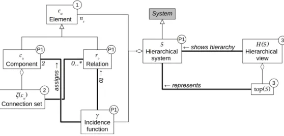
The concepts defined in this section and their relationships are shown in Figure 1 of the appendix.
1.2
The description of the system by an observer
110
We have yet to provide a means to describe elements of our system such that two observers can unambiguously agree on their meaning. Such a description relies on measurement. Measurement itself depends on previous theoretical knowledge, instrument manufacture and on our senses to read and interpret them. All this constitutes a filter between the real world and the knowledge we have of it: measurement is subjective. In order to communicate our experience of real-world objects, we must specify a description that can be shared between
115
Figure 2: Illustration of the hierarchical view of systems S1 (animal), S2(ecosystem), and S3 (landscape) from
Figure 1 according to Definition 3. The hierarchical views, labelled S1′, S1′′, S2′ and S3′, are shown in orange. The top operator enables nesting systems into a hierarchy, by making it possible for a component in the upper-level system to represent a full lower-level system.
Figure 3: Descriptions of system components using Definitions 4-5. Example based on system S2 of
Fig-ure 1. Descriptions, each made of a list of descriptors, are shown for four components and the sys-tem itself. For example, assuming that ‘lion No.1’ is the 1st component of the system, its description is D1(c1) = (d1= id, d2= w, d3= s, d4= a, d5= M, d6= p, d7=□), where id is the label and □
rep-resents a bitmap (for the photo). The description of the whole system (The Namib desert ecosystem) is DS = ((id), (L, l) , P, w, (p1. . . p12)). The structural description (Definition 6) of the system is DS =
(13, (1, .., 13) , 23, (1, .., 23) , ((1, 1, 2) , (2, 1, 3) , .., (23, 13, 11) )). Pictures were downloaded from low-resolution thumbnails on the internet.
propose to attach descriptors (labels, indices, categories, quantities, texts, images, sounds etc., with appropriate units or other technical metadata) to system elements. For notational simplicity, we assume that all descriptors can be represented numerically.
Proposition 2. An observer O is an agent (person, device) able to produce a description D of a hierarchical
120
system, component, or relation. Descriptions constitute the only way for observers to communicate about a system.
Definition 4. Description.
1. The description D (ew) of a system element ew∈ E is a n-tuple of descriptors dx defined by their use and
interest for the observer (cf. Definition 5):
125
D (ew) := (dx)x≤nD
where the index w is the element index in system S. nDis the dimension of the description.
2. Similarly, we define the description of the system D (S), with the convention that D (S) = D (top (S)). Definition 5. A descriptor (d,R) of a system element ewis the association of:
1. d: a n-tuple of numeric variables:
d (ew) := (zy)y≤n
d, zy∈ R
nd is called the dimension of the descriptor.
2. R: an interpretation rule, which associates meaning to d for an observer O. Examples of such rules include measurement units, particular algebraic rules for combining values of different descriptors, coding rules, and any other metadata applying to d.
We assume the rule R is not necessarily expressed in mathematical terms. For this reason, in what follows we denote the descriptor by d only. The particular meaning of each descriptor within a description is apparent
135
in our notations by considering that the description cannot be written simply as a single concatenated list of numeric variables.
See Figure 3 for an illustration of definitions 4 and 5. The description of an element depends on the observer, who has a particular purpose to guide her/his choice. As a result, many descriptions of the same element or system may exist, representing the observer’s interpretation of the system.
140
We now return to Proposition 1, to distinguish between the real world and its representation. Following Tansley (1935), a system is a ‘mental isolate’ of the real world. As system elements belong to the real world, it means Proposition 1 is just a description sensu Definition 4 of the system. Proposition 1 describes the structure of a hierarchical system in mathematical terms. By structure, we mean how components and relations are linked to form an organised system, without any assumption as to what components and relations really are.
145
We acknowledge this through the following re-interpretation of Proposition 1: Definition 6. The structural description of a hierarchical system is
D (S) = (d1, d2, d3, d4, d5) where d1= nc d2= (idC(cu))u≤nc d3= nr d4= (idR(rv))v≤nr d5= (idR(rv) , idC(ci) , idC(cj))v≤n r, γ(rv)=(ci,cj)
and where idA(. . .) is the identifier function over set A: it associates a number to a component or relation that
is unique over their respective sets C and R. d1-d5 are the standard structural descriptors of the system.
Although making the difference between the system and its mathematical expression explicit may seem
150
pedantic, it will be useful when considering: (1) dynamic systems; (2) experiments on real-world systems; and (3), systems which elements are partly unknown.
The concepts defined in this section and their relationships are shown in Figure 2 of the appendix.
1.3
The state of a system and its measurement context
If obtaining values for descriptor variables (zy) (Definition 5) is the act of measurement, then the set of
measure-155
ments of all descriptors of an element is its state at the time of measurement (system dynamics are explored in Section 1.4). In computer science terms, the act of measurement as defined here is an instantiation: the descrip-tor being a class or type definition and the state, an instance of this class with a physical existence somewhere (in computer memory or on a sheet of paper as the case may be). It must be assumed that measurements are
reliable: if they differ, the element is assumed to have changed. For this to hold, measurements must satisfy 160
some robustness principle, such as ergodicity (Boltzmann, 1871) or the law of great numbers (Bernouilli, 1713), which state that the mean of repeated measurements in the same conditions on the same object will converge asymptotically to the same value. The whole theory of sampling statistics (e.g. Cochran, 1977) was developed to solve the problem of how to get a ‘representative’ measure of a real object or system.
Figure 4: Two different local contexts (Definition 7) l21,6 (for descriptor 2 (biomass w ), observer 1, component
6) and l61,6 (for descriptor 6 (mating probability p), observer 1, component 6), computed for focal component c6
(Lion 6) of example system S2(Figure 1). Indexing according to Figure 5. Brown: the full system graph as on
Figure 3; black: the focal component c6; light blue: the relations and components involved in the local contexts.
Local context l21,6groups all the components and relations needed to compute an increase of biomass for lion c6
(component and relation meanings are listed in Figure 1) through feeding: c11is the food source, i.e. a stranded
whale; c1-c4are other lions, one of them (c4) belonging to the same pride as c6; c12is a flock of seagulls attracted
by the carcasse. It is easy to imagine that the share of the food available to the focal lion c6can be the result of
a relatively complex computation / measurement protocol involving all these components and their relations. The newly computed biomass w for lion c6 is its partial state (Definition 9) σ21,6 relative to l21,6 for descriptor d21,6. l21,... is thus the local context relevant to compute biomass increase for lions. Local context l61,6 groups
all the components and relations needed to compute probability of mating between lions: (female) lion c6 is
member of a pride comprising one male c4and another female c5; but while feeding on the beach c10it may be
approached by male lion c1, member of a different pride, and interesting behavioural interactions may result in
birth of lions, i.e. changes in graph structure (Section 1.4). l61,... is thus the local context relevant to compute
Figure 5: Indexing rules. Left, dimensional indexing: each index represents a dimension of a data structure, hence the notation xij. Right, hierarchical indexing: each lower level index in a hierarchy tree depends on the
previous level index, hence the notation xji.
Although the descriptor is attached to an element (Definition 5), hereafter called the focal element, its
165
instantiation may require additional knowledge such as the location of the focal element within the graph representing the system. For example: many plant competition models are based on measures such as the number of neighbour plants in a circle of fixed radius centred on the focal plant; the amount of food gained by an animal may depend on the size of its social group or its position in the social hierarchy; water run-off on a given landscape unit may depend, not just on its elevation, but on its relative position within the landscape
170
(slope, valley, ridge top). All these focal element descriptors depend on its relations with other elements as specified by the system incidence function (Proposition 1). The sub-set of elements required to compute the state of a descriptor of a focal element we call a local context.
Definition 7. The local context l of a focal element ewis the result of applying a graph operator Lwon system
S, that returns a connected (Diestel, 2000) subgraphS′ of S containing ew:
175 l (ew) = S′ := Lw(S) Lw(S) := (Cw, Rw, γw) Cw⊂ CS Rw⊂ RS γw[Rw]⊂ γS[RS] ∄ci∈ Cw| ζ (ci) =∅
where f [A] is the image of set A by function f , and with the additional constraints: 1. if ew is a component ew= cu∈ CS:
cu∈ Cu
2. if ew is a relation ew= rv ∈ RS:
rv ∈ Rv
γv(rv) = (c1, c2)⇒ c1∈ Cv, c2∈ Cv
There may be a unique subgraph for each descriptor. Figure 4 provides an example of two local contexts for Lion 6 in the Namib desert ecosystem of Figure 3: one is used to calculate the biomass of Lion 6 and the
180
second to calculate its mating probability.
Emergence is about comparing microscopic and macroscopic states of the system. The microscopic state involves computing the states of all system elements and combining them in some way into a system-level state. From Definitions 5 and 7, it should be straightforward to compute the state of a single system element. However, much confusion may arise if we consider that: (1) elements may have different descriptions, i.e. different sets
of descriptors, with different sets of variables; (2) different observers may define different descriptions, and even a single observer may wish to work with different descriptions of the same element; (3) the method used to compute a local context may depend both on the particular element considered and on the particular descriptor. To denote the dependency on all these families of objects (observers, elements, descriptor variables), we will use rigorous indexing rules (Figure 5): Dmwindicates that the description of an element ewdepends on the element’s
190
individuality within the system (index w) and on the observer or the observer’s choice (index m) (Figure 4). Since the descriptors are nested within descriptions (Definition 4), they will be denoted by dxmw, and since descriptor variables are nested within descriptors, they will be denoted by zyxmw. Dimensions of descriptions and descriptors now become nDmw and ndxmw. The local context being used to measure or compute the state of an element and for a particular descriptor, must match the descriptor, and hence is denoted by lxmw. Finally,
195
it makes sense to group the local contexts which will be used to compute the description of a single element: Definition 8. A context q is a n-tuple of local contexts applying to the same focal element:
q (ew) = (li(ew))i∈N
In the Figure 4 example, we may associate the two local contexts defined for computing biomass and mating probability of Lion 6 into the same context: q (c6) =
(
l21,6(c6) , l61,6(c6)
) . With this settled, we can now compute element and system states:
200
Definition 9. The partial state σxmw of an element ew, relative to a local context lxmw, for descriptor dxmw associates an element and a local context with a descriptor instance:
σxmw : E × G (W ) → R ndxmw (ew, lxmw(ew)) → dxmw = ( zyxmw ) y≤ndxmw
where w ≤ ne is the element index, m the observer index, x≤ nDmw the descriptor index in description
Dmw, y≤ ndxmw the variable index within descriptor dxmw.
Definition 10. The local state σmw of an element ewrelative to a context qmw, for description Dmw is defined
205 as: σmw : E × (G (W ))nDmw → Rnmw (ew, qmw) → Dmw(ew) = (σxmw)xmw≤nDmw = ( (zy)y≤n dx ) x≤nDmw where nmw= nDmw∑ xmw=1
ndxmwis the total number of descriptor variables in description Dmw; qmw=
(
(lx)x≤nDmw
)
mw
is the context grouping all the local contexts lxmw used to compute partial states σxmw of descriptors dxmw of description Dmw.
Among all possible subgraphs required to compute a local context, two extremes exist: those that require
210
no other elements and those that require all other elements to be considered.
Definition 11. The minimal local context l0 of a focal element ew is the local context of this element in
isolation:
1. for a component:
l0(cu) = ({cu} , ∅, 0)
where ∅ is the empty set and 0 the null function
215
(a) for a relation:
l0(rv) = ({c1, c2} , {rv} , γ (rv) = (c1, c2))
Definition 12. The maximal local context lS of a focal element ew is the whole system S:
∀ew∈ S, lS(ew) = S
By construction (Definition 3), when choosing a system we isolate it from the rest of the world. Therefore, no local context, other than the minimal local context is relevant at the system level:
220
Definition 13. The system local context is the minimal local context of top (S):
l (top (S)) := l0(top (S)) = ({top (S)} , ∅, 0)
Definition 14. The disconnected state σw of an element ewis its local state relative to the minimal context q0:
σw(ew) = D0w(ew) = σ0w(ew, q0)
We can now define the system microscopic and macroscopic states:
Definition 15. The macroscopic state, or macro-state, of a system Ω (S) is the disconnected state of the component representing the whole system in its hierarchical view (Definition 3):
225
Ω (S) = σ0(top (S))
assuming the component index 0 is attributed to top (S). Even if the observer has not defined any description for the system as a whole, the structural description (Definition 6) always exists. Therefore, any system has at least one macro-state.
Definition 16. The microscopic state, or micro-state, of a system is defined as the n-tuple:
ωm(S) = (σmw(ew))w≤ne
Contrary to the macro-state, the micro-state is not a single description taking some measured values, but a
230
n-tuple of descriptions of all the elements of the system, measured or computed for a particular n-tuple of local contexts that depends on observer m. There may be many micro-states for the same system, depending on the observer’s choices.
Definition 17. The disconnected micro-state ω0of the system S is the micro-state computed using the minimal
context q0 for all elements:
235
ω0(S) = (σw(ew))w≤ne
With these definitions, the emergence problem can be restated simply as: is there a function (to keep it simple; it may be an algorithm or some more elaborate transformation) that links the macro-state and the micro-state(s) of a system? Emergence will depend on the existence and nature of this function.
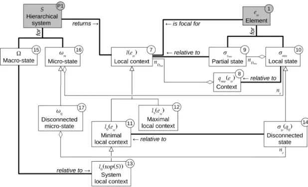
The concepts defined in this section and their relationships are shown in Figure 3 of the appendix.
1.4
System dynamics
240
So far, only static systems have been considered. We now turn to dynamic systems: systems that change over time. We follow the definition of a dynamic graph by Harary & Gupta (1997).
Definition 18. A dynamic hierarchical system is defined as:
S (t + ∆t) = g (S (t) , ∆t)
Two kinds of change may affect the system: changes in structure and changes in state.
245
1. Changes in structure involve creation and deletion of components and relations. We define a structural change as a triplet of sets:
Definition 19. A structural change in the system between times t and t + ∆t is defined as ∆S (t, ∆t) :=(∆S+(t, ∆t) , ∆S−(t, ∆t) , ∆Sγ(t, ∆t))
where
• ∆ denotes any, possibly large, change; 250
• ∆S+(t, ∆t) is the set of elements added to the system (creation set );
• ∆S−(t, ∆t) is the set of elements removed from the system (deletion set );
• ∆Sγ(t, ∆t) is the set of incidences of new relations over components (new branching set ) at time t
over ∆t.
We further define, from Proposition 1, and omitting (t, ∆t) for notational simplicity, ∆C+, ∆C−,∆R+
255
and ∆R−, as, respectively, the set of components added to and removed from, and the set of relations added to and removed from the system between time t and t + ∆t. By construction ∆S+ = ∆C+∪ ∆R+ and ∆S−= ∆C−∪ ∆R−. With these sets defined, the new structure of the system is computed from
C (t + ∆t) = C (t)∪ ∆C+\ ∆C− R (t + ∆t) = R (t)∪ ∆R+\ ∆R− γ [R (t + ∆t)] = γ [R (t)\ ∆R−]∪ ∆Sγ
where \ stands for set substraction.
Since graph elements are discrete objects, a structural change can be reduced to a set of elementary
260
structural changes of at most four types. By elementary, we mean atomic, i.e. a change that cannot be
smaller and occurs instantaneously. We use δ to denote such changes.
Definition 20. An elementary structural change in system δS = (δS+, δS−, δSγ), is one of the four
following changes
(a) deletion of a single relation rv – The deletion set contains only a single relation δS− = δR− =
265
{rv} ⊂ R (t):
δSr−= (∅, {rv} , ∅)
(b) creation of a new relation rv between two existing components ci and cj – The creation set
contains only a single relation to add to the system δS+= δR+={r
v}. In addition, the components
to be connected by this relation must be specified and the incidence function modified accordingly:
δSr+= ({rv} , ∅, {(ci, cj)})
with ci∈ C (t) and cj∈ C (t).
270
(c) deletion of an existing component cu – The deletion set contains the component plus its
con-nection set: δC−={cu} ⊂ C (t) and δR−= ζ (cu):
δSc−= (∅, {cu} ∪ ζ (cu) ,∅)
(d) creation of a new component cu – The creation set contains the new component plus a new
{cu}, with cu∈ C (t), and δR/ += ζ (cu). ∆R+might be empty if the new component is disconnected
275
from the rest of the graph. Information must be provided on how the new component is to be connected to other components. The new branching set is δSγ = γ [ζ (c
u)]. The structural change
becomes:
δSc+= ({cu} ∪ ζ (cu) ,∅, γ [ζ (cu)])
Adding and deleting components and relations atomically in a graph is, therefore, not as straightforward as it might seem. The operation of removing a relation or adding a disconnected component acts on only
280
one object. In all other cases (2, 3 and 4 above), additional information is required. 2. Changes in state affect values of descriptors of components, relations, or the system itself:
Definition 21. A state change ∆σmw(t, ∆t) for an element ew(t) relative to the context qmw(t), is
defined as a change in numeric values of its descriptor variables zyxmw between two successive local states
σmw obtained at times t and t + ∆t (Definition 10) :
285 ∆σmw(ew(t) , qmw) (t, ∆t) := (( zyxmw(t + ∆t)− zyxmw(t) ) yxmw≤ndxmw ) xmw≤nDmw
A similar definition applies to the system as a whole by using its description.
Definition 22. We define dσmw, dωm, and dΩ as, respectively: an infinitesimal change in local,
micro-and macro-state. Infinitesimal means the smallest possibly observable, measurable, or computable change in state as dt approaches zero.
Definition 23. We define an elementary change in system dS as either an atomic structural change δS, or an
290
infinitesimal state change (dωmor dΩ). In both cases, dS is the smallest possible change a system can undergo.
Changes in structure are discrete by nature (section 1.4), because components and relations are discrete system elements. Hence discrete-time and event-driven models may better manage structural changes (Zeigler et al., 2000). Changes in descriptor values may be discrete or continuous. It follows that models describing the dynamics of a hierarchical system must allow for both continuous and discrete change. Coupling differential
295
equations with a discrete-event logic is a difficult task that has been explored mainly by simulation specialists (e.g. Duboz et al., 2003).
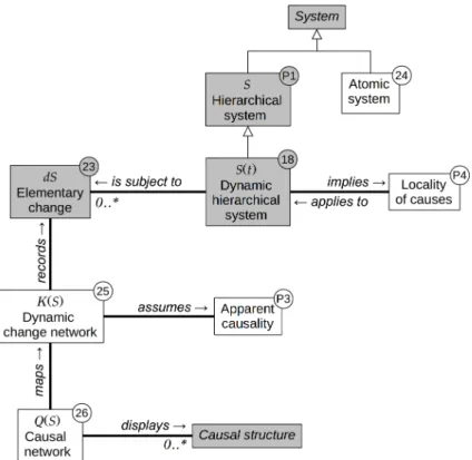
The concepts defined in this section and their relationships are shown in Figure 4 of the appendix.
1.5
Causality
It is not our aim here to enter a philosophical debate addressing the reductionnist vs. holistic dispute, or the
300
mechanistic vs. empirical modelling issue. In this framework, a cause is what produces a change in system state. In general, dynamics, as an observed succession of changes, does not inform about the underlying causes. System dynamics may be described in many ways, e.g. by a set of differential equations linking system variables, stochastic markovian transitions, deterministic rules, etc. – there is usually some debate about whether these methods represent real causes or are just phenomenological descriptions of dynamic changes. However, a
305
recurrence equation such as that of Definition 18 implies a form of causality, as it assumes that the state of the system at time t + dt can be computed from its state at time t. This satisfies a necessary condition for causality: a cause must, by definition, precede the effect. We propose here to assume that this condition is also sufficient under the condition that dt represents the smallest amount of time at which we are able to see a difference in system states. In this case, nothing can be said about what happened between t and t + dt,
310
and rather than saying that either (1) some complicated speculative process occuring within this time period caused the change, or (2) what we observe is only correlation, we assume that the state at time t caused the state at time t + dt. This is an application of the parsimony principle: in the absence of better information on the system functioning, at a chosen time grain the recurrence equation of Definition 18 describes some form of causality that we call apparent :
Algorithm 1 Pseudocode for the propagation of changes in an atomic system (Definition 20). generateChange(S (t),t,dt) { return(dS (t, dt)) } changeSystem(S,dS,t,dt) { S (t + dt) := some_computation(S (t),dS (t, dt)) } propagateChanges(S,t0) { t := t0
while (stopping_condition(t,S) is false) { ... compute dt ... dS := generateChange(S,t,dt) changeSystem(S,dS,t,dt) t := t + dt } }
Proposition 3. Apparent causality: If S is a dynamic system sensu Definition 18 and if dt is an infinitesimal
atomic duration (called time grain) then we postulate that S (t) is the apparent cause of S (t + dt) at time grain dt.
We consider that apparent cause is the best approximation of real cause given the information we have on the system.
320
Often, the dynamics of a system is represented by a set of coupled recurrence equations (e.g. differential equations) applying to a set of variables. In our framework, such a set of variables is what we have called the description (Definition 4) of a component, relation or system. In other words, this common use of recurrence equations does not apply to our hierarchical system, but to a simpler system or object:
Definition 24. Atomic system. A system S is atomic if it cannot be subdivided into elements. Such a system
325
is non-hierarchical.
An atomic system can have a description (Definition 4).
The recurrence equation applies to an atomic system as a whole. As a consequence, changes in system state result from each other: if we link changes through the causal relation implied by the recurrence equation, we will obtain a simple chain of change events. This is sometimes called linear causality1, as the common reductionnist
330
view is to identify changes with causes, specially as dt→ 0. For a better understanding and later comparison, we provide the trivial pseudocode (Algorithm 1) for the case of the atomic system.
In a hierarchical system, this simple scheme no longer applies, as system elements may be subject to their own dynamic recurrence equation. Let us first consider a graph which only undergoes state changes (Defini-tion 21) but no structural changes (Defini(Defini-tion 19) and, for simplicity, that these changes are driven by differential
335
equations (among other possible methods) to describe a dynamic. Can we rewrite the recurrence equation of Definition 18 in order to account for graph structure? It may be possible to re-organise it into a system of equations applying to components and relations. But this ignores graph structure and treats the graph as an unstructured list of elements. It is difficult to imagine a graph component affecting another without there being a relation between them – otherwise, by definition, the graph is not a correct representation of the observer’s
340
system. To be consistent with our initial assumption (Proposition 1), that a graph is the correct way to repre-sent a hierarchical system, we postulate that the graph architecture must be used in dynamics computations in a meaningful way. We propose the following to impose this consistency:
Proposition 4. Locality of causes: in a dynamic hierarchical system, elementary dynamic changes are produced
and successively spread following system relations and components, i.e. locally. 345
Algorithm 2 Pseudocode for propagation of elementary changes over the system graph. generateChange(ec,σck(t),lk(t),t,dt) { return(dec(t, dt)) } neighbours(ca) { return({rj} |γ (rj) = (ci, ca)i≤nc) } neighbours(rb) { return({ca} |γ (rb) = (ci, ca)) } // recursive updateElement(ec,k) { newContext := some_computation(lk(ec)) newState := some_other_computation(newContext) if (newContext̸= lk(ec) or newState̸= σck(ec)) { lk(ec) := newContext σck(ec) := newState for (ed in neighbours(ec)) { updateElement(ed,k) } } } changeElement(ec,k,dec,t,dt) { lk(ec(t + dt)) := some_computation(lk(ec(t)),dec(t, dt)) σck(t + dt) := some_other_computation(lk(ec(t + dt))) for (ed in neighbours(ec)) { updateElement(ed,k) } } propagateChanges(S,t0,k) { t := t0
while (stopping_condition(t,S) is false) { ... compute dt ... for (c := 1 to ne) { dec := generateChange(ec,σck(t),lk(t),t,dt) changeElement(ec,k,dec,t,dt) } t := t + dt } }
This means that the dynamic recurrence equation of Definition 18 has a causal meaning only if applied at graph element level; the system-level recurrence equation will be the result of these local dynamic equations. The algorithm needed to compute changes and propagate them over the graph becomes more elaborate, involving recursion (Algorithm 2).
At each granular time step, elementary change (Definition 23) may arise due to element local context
350
(Definition 7) and state (Definition 10). Focusing on only one of these changes, once applied, it will in turn at the next granular time step trigger its elements’ neighbours (outgoing relations for components, end component for relations) to update their own local context and state accordingly; if this results in a change of local context and state, the process is further propagated to the graph network until there are no more changes in local context and state. This sequence describes the spread of changes from only one element. However, many
355
changes could arise simultaneously from many different elements, generating overlapping spreading networks of changes, generating possible conflicts and interactions between them. The algorithm does not specify how changes are generated: it merely assumes changes may be generated using the information available to the observer of a given system element, i.e. its local context and state. With an appropriate method to generate
changes, the system might start evolving simply due to its initial micro-state.
360
In Algorithm 2, it is theoretically possible to find the changes that have been caused by other past changes by tracking the succession of local context and state updates that caused the generateChange() function to generate it. Elementary changes can then be chained, possibly forming a network of changes apparently caused by each other (Proposition 3). This is a long way from the simplicity of linear causality. For the analysis of system dynamics, it is helpful to define the following graph:
365
Definition 25. A dynamic change network of a dynamic hierarchical system K (S) is a directed graph describing the causal pathways between elementary changes of a realised system dynamics (S (t))t<∞under the assumption of apparent causality. Its components and relations are defined as follows:
1. To each node vi∈ CK is attached a description with four descriptors :
DK(vi) = (di1, di2, di3, di4) where di1= idCK(vi) , vi∈ CK di2= idCS(ew) , ew∈ ES di3= t di4= dS di5= dt
di1 is the unique identifier of node vi in graph K (S), ES = CS∪ RS is the set of elements of S , di2
370
the unique identifier of element ew in system S, di3 is the time at which the change occured, di4 is the
elementary change in S, and di5 is the time grain.
2. The directed edges of K (S) reflect the direction of apparent causality (Proposition 3), a → b meaning that a caused b. They have no descriptor variable except their unique identifier. They link nodes that differ at successive times separated by the time grain dt :
375
γK : RK → CK× CK
rv → (vi, vj)| (di3= t) and (dj3= t + dt)
The dynamic change network of a dynamic system provides an image of the succession of changes that occur during a particular dynamic (Figure 6). Since time increases on every edge, there is no possibility to loop back in such a network, which is thus an oriented graph (Diestel, 2000). However, since the causal pathways may involve loops (system elements affected more than once over the time course of the dynamics) and conflicts (more than one change occurring on one element at the same time), it may be useful to make them visible by
380
’projecting’ the dynamic change network back on the initial system:
Definition 26. A causal network of a dynamic system Q (S) is a graph operator mapping a system dynamic change network K (S) on the system S, where there is one node c′wfor every element ew of S :
CQ={c′w}w≤ne
Figure 6: Example of a dynamic change net w ork K (S ) and its causal net w ork Q (S ) asso ciated to a simple system S . These net w orks reflect the cascade of changes o ccuring after a single initial change in one comp onen t of the system. T op : successiv e states of S along a dynamics (from time t = 1 to 10 ); ra ys around a comp onen t: change on that comp onen t; straigh t arro w: change on a relation; curv ed arro ws: structural changes, created or deleted elemen ts app earing as dotted lines. Midd le : the dynamic change net w ork K (S ), recording all changes on S ; K (S ) no de: an elemen t of S sub ject to a change at a giv en time step; K (S ) link: the causal link b et w een the changes according to the lo calit y of cause principle (Prop osition 4); the four en tries for eac h no de represen t the first four descriptors of Definition 25 (the fifth descriptor, time step, is assumed constan t, hence not sho wn). Bottom: K (S ) is folded o v er itself to yield the causal net w ork Q (S ), where a unique no de is k ept for ev ery elemen t of S , and where links of K (S ) are merged in to single links with a m ultiplicit y (Definition 26), sho wn as a n um b er on ev ery link of Q (S ). The dotted arro ws b et w een K (S ) and Q (S ) sho w ho w links of Q (S ) are built in tw o particular cases (for the c3 → c3 link and the c1 → r2 link, whic h o ccured twice in K (S ), resulting in a m ultiplicit y of 2 in Q (S )).
descriptor, i.e. refer to the same element of S. We use the merging function h to build the edges: 385 h : RµK → RQ M = {rv| γK(rv) = (vi, vj)} → rv′ | γQ(rv′) = ( c′w1, c′w2) with di2(vi) = idES ( c′w 1 ) and dj2(vj) = idES ( c′w2 )
We associate to each edge rv′ of Q (S) a descriptor called the multiplicity µ, which is the number of edges of
K (S) used to construct it: µ =|M |, where |A| denotes the cardinal of set A. This will indicate which causal
pathways are most frequently used over a particular dynamics. By construction,
|R∑Q|
i=1
µi=|RK|.
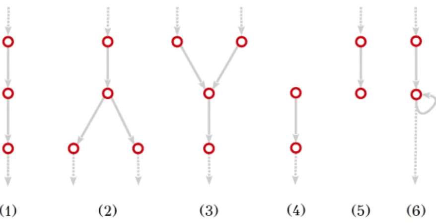
Causal networks contain causal patterns other than simple linear patterns (Figure 7). Due to these patterns, the system dynamics may become extremely difficult to track, predict, or understand from a mechanistic point
390
of view. This issue, characteristic of hierarchical systems, has long been identified as a major feature associated with emergence (e.g. Bedau, 2003; de Haan, 2006; Searle, 1992; Kim, 1992).
The concepts defined in this section and their relationships are shown in Figure 5 of the appendix.
Conclusion: the hierarchical system ontology
While the definitions proposed so far are not necessarily original, we have: (1) made them precise; (2) organised
395
them in a logical progression; and (3), used only the indispensable backbone of the hierarchical system in order to see where and how emergence arises within this set of concepts. Our hope is that this ontology will help to clarify inter-disciplinary discussion of hierarchical systems.
2
Where does emergence lurk?
There is no single, agreed upon, definition of emergence (e.g. Bar-Yam, 2004; Bedau, 2003, 2008; Chen et al.,
400
2009; Cotsaftis, 2009a; Crutchfield, 1994; Kim, 1999; Muller, 2003; Searle, 1992), but syntheses have been proposed (Bedau & Humphreys, 2008; de Haan, 2006; Bonabeau & Dessalles, 1997). Three major types of emergence were proposed by de Haan (2006): (1) observer-induced emergence, but without consequences for the system itself, that he called discovery; (2) mechanistic emergence, with real consequences for the system independent of the observer; and (3) reflective emergence, where the observer is actually part of the system
405
and may affect its dynamics (something that Muller (2003) calls strong emergence). Most authors develop similar classifications, e.g. (Assad & Packard, 1992) distinguish four types of emergence on a scale of increasing ‘objectivity’; terms of ‘weak’ and ‘strong’ emergence are often used, although with different definitions (e.g. Bedau, 1997; Muller, 2003; Searle, 1992).
From our ontology, we identified four types of emergence that match precise properties of the hierarchical
410
system defined as a graph (Proposition 1). We do not claim these four types are exhaustive, but they address the most often encountered meanings of emergence. One we do not address is the reflective emergence sensu de Haan (2006) or strong emergence sensu Muller (2003), i.e. the case where the observer is part of the system. In our ontology, the position of the observer relative to the system is irrelevant. We formulate precise definitions of emergence in terms of the system properties they imply. The first three definitions depend on the presence
415
of the observer (Proposition 2) and the last applies only to dynamic systems (Definition 18).
2.1
‘Trivial emergence’ due to ignoring system integration
The definition of complex systems and emergence are often linked. Typically, a system is said to be complex if it displays ‘properties that emerge from interactions between its components’. This just means, in our formalism, that a set of components is different from a graph. The difference lies in the relations and the incidence function
420
One should avoid reducing a hierarchical system merely to the set of its components, but this seems to be common practice (Cotsaftis, 2009b). The popular statement that ‘the whole is more than the sum of its parts’ is just the (not very surprising) observation that relations are important. Many multi-agent systems focus on the
control problem: they consider that emergence arises when the interactions between agents are not controlled 425
by a central or external force (systems that Cotsaftis (2009a) calls ‘complicated’). This is equivalent, in our case, to systems where the incidence function γS is not known a priori, but is generated by system dynamics
from individual component behaviours. To distinguish those hierarchical systems that are simple enough to understand without being concerned with relations, from those where this information is important, we define two new terms:
430
Definition 27. A flat system is a system in which the only micro-state is the disconnected micro-state:
∀m ∈ {1...M} , ωm(S) = ω0(S)
Neither local contexts nor interactions play any role in the micro-state computation: the system is ‘flat’,
i.e. displays no structure. It is nothing more than the set or the disconnected graph of its components:
S =
(
{cu}u≤nc,∅, 0 )
≡ {cu}u≤nc.
On the example of Figure 4, the flat micro-state of S2 would ignore the local contexts l21,6 and l61,6. In the 435
case of l21,6, it means that access of Lion 6 to food would not depend on the presence of other lions. This is
synonymous to an absence of competition for food and comparing ω0(S2) and ω1(S2) would be a measure of
this competition.
Definition 28. An integrated system is a system which verifies
∃m ∈ {1...M} | ωm(S)̸= ω0(S)
Since we can compute the disconnected micro-state (Definition 17) of any system, we can measure the
440
importance of relations, which we call integration I of the system, by comparing its micro-state to its flat micro-state using some measure of distance:
Definition 29. System integration Im(S) is defined as the distance between ωm(S) and ω0(S):
Im(S) = ne ∑ w=1 n∑Dmw xmw=1 ndxmw ∑ yxmw=1 zyxmw− zyx0w
where∥. . .∥ denotes some distance defined on R+. For the flat system,I
0(S) = 0.
We can then state:
445
Definition 30. A system is said to display trivial emergence if
∃m ∈ {1...M} | Im(S) > 0
When the terms ‘complex system’ and ‘emergence’ are used in this usual, ‘naive’ sense, we suggest using definitions 28 & 30 instead, as those both refer to some observer surprise at novelty which is not really new: it’s just that an important part of a system has been ignored. Here, trivial emergence is an indication of unaccounted for system integration, i.e. the importance of the relations and incidence functions in computing
450
the system micro-state. By construction, any non-flat hierarchical system has trivial emergence, which makes this concept uninformative within the present formalism.
2.2
Emergence due to the observer’s choice of descriptors: discovery
Even after accounting for system integration, observers may build a model that, to the best of their knowledge, represents accurately their understanding of the system under study. However, after further analysis, they find
that the behaviour of their model and the real system diverge. The observer then realises that the model may be revised to reduce this discrepancy. This is what Bonabeau & Dessalles (1997) call emergence relative to a
model : the system displays an unexpected property, that was not observed when the model was constructed.
This emergence is observer- (model-) dependent and transient, as it will disappear when the model is revised to account for the formerly emergent property. Should we use the name ‘emergence’ to only differentiate between
460
unexpected and expected results in the routine process of experimental science? We agree with Crutchfield (1994) in calling this kind of emergence discovery, which implies the idea of being part of a dynamic process. Contrary to emergence, discovery is an event in time. Before the discovery, the unexpected properties seem emergent simply because they are unexplained; after the discovery, with the improved model of the system, their emergent character vanishes.
465
Definition 31. Discovery is defined as an event (at step 6) in the following process:
1. an observer O of a system S expects the system dynamics to match some predefined pattern, i.e. a particular time series of states θ = (Ω (t) , ωm(t))t<∞, where m denotes the method chosen by the observer
to generate the micro-states, according to some previous knowledge;
2. O chooses system and element descriptions DS and (Dmw)w≤neassumed to appropriately describe the
470
system in order for its dynamics to display the pattern;
3. using some measurement or computation technique,O generates a realised dynamic series of system states ˆ θ = ( ˆ Ω (t) , ˆωm(t) ) t<∞ ; 4. O uses an error function ϕ
(
θ, ˆθ
)
to compute a distance between the realised system dynamics and the expected pattern;
475
5. based on some tolerance threshold τ , O then decides that the realised dynamics does not match the expected pattern when ϕ
(
θ, ˆθ
)
> τ ≥ 0. We call this event the observer surprise in front of unexpected results;
6. Using another set of descriptions {
D′S, (Dmw′ )w≤ne }
, and repeating steps 3-4, we call discovery of a better
description of the system the fact that ϕ
( θ′, ˆθ′ ) < ϕ ( θ, ˆθ ) ; 480 7. Furthermore, when ϕ ( θ′, ˆθ′ ) < ϕ ( θ, ˆθ ) but ϕ ( θ′, ˆθ′ )
> τ ≥ 0, the discovery is incomplete as there is a
possibility to further improve system description beyond the current improvement.
If the realised dynamics matches the expected pattern at step 5, or if the observer does not try another set of descriptions at step 6, there is no possibility of discovery.
Let us now imagine that we have discovered all the descriptors needed to understand a system. It may well
485
be that the system and its elements have completely different descriptors, that mean completely different things (in Definition 4, each element can have a different description, i.e. a different set of descriptors). Bedau (2003) defined nominal emergence as the case where system-level properties have no counterpart at the component level because this would not mean anything, like the concept of the speed of an object in a movie has no meaning when individual frames are taken separately. However, he also explains that nominal emergence is a
490
‘first approximation’, a very broad concept that only points to a discrepancy between macro- and micro-level descriptions of a system, without further explanation. Here, nominal emergence arises naturally from Definition 4.
Finally, we might find that the macro-state of a system is a much ‘simpler’ description of the system than its micro-state. Dessalles et al. (2007) formalised this case as ‘emergence relative to a model’ (but with a different
495
meaning from Bonabeau & Dessalles (1997)). It is based on the observation of a drop in complexity (using some mathematical definition of complexity, such as algorithmic complexity) between the higher-level observations of a system behaviour (the macro-state) and the detail of the rules generating those observations (the micro-state).
For example, in J.H. Conway’s game of Life (https://en.wikipedia.org/wiki/Conway’s _Game_of_Life), one may observe that the patterns called gliders reproduce themselves every four timesteps at a certain distance
500
and in a certain direction, which produces the illusion of movement. One can then describe a glider by giving the position of the cells for the first four time steps and say that this sequence continues as long as the glider ‘lives’. This is a description of a glider that is in general shorter than listing the positions of the cells that constitute the glider for its entire lifespan. The shorter description requires a macroscopic point of view from the observer to recognise spatial patterns and relate together patterns that are several timesteps apart. The
505
description, being shorter, represents a drop in complexity.
2.3
Emergence due to computational irreducibility between macro-state and
micro-states
In sections 2.1-2.2, emergence could be attributed to a lack of information about the system. However, if we assume perfect knowledge, emergence may still be manifest as a gap between system macro- and micro-state.
510
We formalise this gap through the following question: is there a function such that the macro-state can be computed from one of the micro-states?
Definition 32. The upscaling function relative to a context qm is defined as:
fm: Rnm1× . . . × Rnmne → RnDS
ωm(S) → Ω (S)
fm allows two nested organizational ‘scales’ or levels to be related: the system (upper level/scale) and its
elements (lower level/scale).
515
Emergence can be defined from the properties of the upscaling function:
1. fmexists – According to Kim (1999), there is no emergence if the upscaling function exists. The
macro-state simply results from its micro-macro-state(s). It is nothing more than a computation based on the system elements, no matter how convoluted that computation may be.
Other authors (Bedau, 1997; Searle, 1992) consider that the difficulty of the computation does make a
520
difference: when the computation of the macro-state is particularly difficult (Bedau, 2003), the system is said to be weakly emergent. Zwirn & Delahaye (2013) formally define computational irreducibility2 to
specify what is meant by ‘particularly difficult’. Other authors are very unclear on this topic. Informally (and using our definitions 15 & 16), computational irreducibility means that there is no way to compute Ω (S) from ωm(S) without having to compute every state of every element in turn; in other words, fm
525
cannot be simplified: every detail of the system matters.
2. fmdoes not exist – Assad & Packard (1992) rate this circumstance at the top of a scale of four increasing
degrees of emergence and call it maximal emergence: the macro-state cannot be deduced from the micro-state by nature.
Our definitions of micro-state, macro-state and upscaling function, while mapping relatively well to existing
530
concepts of emergence, nevertheless raise new questions.
Authors defining weak emergence usually consider only system ‘components’ without explicitly including relations and incidence functions in their system definition (cf. Section 2.1). Therefore, it is difficult to know to what parts of the system computational irreducibility should apply. There appear to be two options:
1. Computational irreducibility interpreted stricto sensu, i.e., the computation of the macro-state must
535
include all the details of the system. We interpret this as meaning that the only relevant context is the maximal context qS. The condition for weak emergence is then:
2Zwirn’s definition of computational irreducibility is based on Turing machines (Zwirn & Delahaye, 2013), but he states in this
article that a similar definition could be proposed based on functions. We assume here that such a definition exists, functions being easier to include in the present formalism.
Definition 33. Weak emergence occurs when the only existing upscaling function is based on qS and is
computationally irreducible sensu Zwirn & Delahaye (2013):
∃fS ̸= 0 | Ω (S) = fS(ωS(S)) , and fSis irreducible
∄m ∈ N | Ω (S) = fm(ωm(S))
where 0 stands for the null function.
540
2. Computational irreducibility interpreted more loosely:
Definition 34. Context-dependent emergence occurs when the upscaling function fmis computationally
irreducible sensu Zwirn & Delahaye (2013):
∃m ∈ N | (Ω (S) = fm(ωm(S))) and fmis irreducible
Here we make no assumption about other contexts as context-dependent emergence applies only within this specified context m. The system may well be non-emergent using other local contexts.
545
With the upscaling function, we can explicitly link weak emergence (Bedau, 1997; Searle, 1992) to computational irreducibility, as claimed by Zwirn & Delahaye (2013). Our explicit representation of the system as a graph enables us to distinguish between a weak emergence independent of local context and a context-dependent weak emergence, which depends on how micro-states are built with respect to local context. Definition 34 is useful when only one non-trivial local context is available to compute the micro-state, a probably common case
550
compared to the requirements of Definition 33 where all local contexts must be assessed.
The case where an upscaling function does not exist is difficult to interpret: it is hard to imagine this possibility without it being a case of missing descriptors, as in discovery (Definition 31). If this is not the case, how should we interpret this kind of emergence, usually qualified as strong? Could a system, with a macro-state that cannot be explained from its micro-state, exist? To diagnose strong emergence in a system would mean
555
that there is no way to explain its macroscopic behaviour (or some part or it) from its microscopic description. It would mean that any scientific enquiry to explain the macroscopic behaviour from the parts would be doomed to fail. Conversely, any attempt at explaining the macroscopic behaviour from the parts assumes that the system does not display strong emergence. Quoting Bedau (2003):
Strong emergence starts where scientific explanation ends.
560
Short of having any evidence of being in presence of strong emergence, and as long as we are willing to keep trying to explain the macro-state from the miscro-state, we are left with the assumption that strong emergence does not exist. In our formalism, this translates to assuming:
Proposition 5. A hierarchical system always has at least one upscaling function:
∀S, ∃ (Ω, m, ωm, fm)| Ω (S) = fm(ωm(S))
If the upscaling function cannot be found using the current system description, then new descriptors must
565
be added to the description until a satisfactory upscaling function can be written.
In accordance with our present scientific approach of the world, we therefore assume that maximal emergence
sensu Assad & Packard (1992) does not exist. We expect system-level and subsystem-level descriptions to match
somewhere – even if this ‘somewhere’ is very difficult to find. If they do not, it means something is missing in the description of either or both levels.
570
2.4
Emergence due to complex causality networks
Integration, discovery and computational irreducibility, considered as forms of emergence by many authors, do not require the system to be dynamic. However, many specialists of emergence base their definitions on
causation, implying a dynamic system (Bedau, 2003; Kim, 1992). For Bedau (2003) and Searle (1992), downward
causation (i.e. the system causing its elements to change) that is not reducible to upward causation (i.e. changes 575
in the system being caused by its elements) is called strong emergence. However, they believe strong emergence does not exist in nature. In contrast, for Muller (2003), the distinction between weak and strong emergence depends on downward causation from the system on its components by (1) merely affecting their behaviour (weak) or (2) changing the rules of their behaviour (strong). It seems that in all cases, including Kim (1999), emergence is associated with the difficulty in predicting the system’s behaviour because of complicated causal
580
pathways. Although there is clearly no agreement on how emergence relates to causal pathways, there seems to be a tendency to admit that (1) the microscopic control of dynamics is the ‘normal’ causal pathway, i.e. the system macro-state is supervenient to its micro-state given some context, and is (weakly) emergent when the upscaling function fmis computationally irreducible (Definitions 33-34); and (2) any macroscopic control of
the dynamics is reducible to the microscopic dynamics, i.e. there is a causal loop from the micro-states to the
585
macro-state and back to the micro-states.
There are problems with these definitions: (1) they tend to focus on components to the exclusion of relations; relations could also have causal powers; (2) there may be a wide diversity of causal powers among components and relations, i.e. they may generate structural change events, or drive smooth changes in descriptor variables, or just change passively in response to stimuli from other components or relations; and (3) they ignore the
590
potentially very high complexity of causal networks (Section 1.5), where causal pathways may cross and interact in very elaborate ways, generating particular causal circuits (Figure 7). These ideas may be present, but only
implictly in most articles. Making the causal network explicit (Definition 26) is our answer to these complex
causality issues: what could happen may be so intricate that the notions of downward or upward causation just become obsolete because they are incapable of capturing such complexity.
595
Research in cybernetics (Wiener, 1948) and biology (Weiss, 1971) has for some time recognized the ability of feedback loops to disrupt the linear chain of causality by having an effect acting back upon its cause. Patten & Odum (1981) identified two different ways of constructing feedback loops within a cybernetic system. For Bateson (1972, quoted in Ulanowicz, 2009), causal circuits can react non-randomly to random events. Electronic engineering routinely uses feedback loops of various types to design complex regulatory systems (control theory:
600
Astolfi et al., 2008). The causal loop is considered the first step towards self-organisation (De Wolf & Holvoet, 2005). Cotsaftis (2009b) considers that a system is complex when ‘self-organisation filters out external action, making the system more robust to outer effects’. In ecology, Ulanowicz (1990) builds upon this result to demonstrate that feedback loops in trophic networks disrupt the overwhelming physical linear causation to yield a different logic, where the stability of cycles arises from a constant throughput of energy or matter. His
605
reasoning is based on the energy and matter flows in trophic webs. Ulanowicz (2009) further demonstrates that some loops may be stable and constitute kernels of coherence in a system. In all these works, loops are able to acquire a predictable and deterministic-like behaviour from randomness, and remain partly autonomous from external forcings. The weakness of all these works, however, is that most of them cultivate an ambiguity between flows and causes: there is a semantic drift from flow loops to causal loops in their vocabulary.
610
Here, we solve this ambiguity by explicitly building, for any dynamic hierarchical system, a causal network (Definition 26). The causal network itself is a particular case of a flow network (Diestel, 2000), so that all the previously mentioned cybernetic and flow dynamics results apply. Our formalism gives them a much broader scope. Not only matter and energy flows, but any other type of graph dynamics, including structural changes (component and relation addition and deletion: cf. Definition 19, 20), can be considered.
615
What is the relation between (stable) causal loops and emergence? According to Bedau (1997), emergence has two ‘hallmarks’:
(1) Emergent phenomena are somehow constituted by, and generated from, underlying processes; (2) Emergent phenomena are somehow autonomous from underlying processes.
Autonomy is the key word. According to cybernetics, stable causal loops are able to provide some autonomy 620