HAL Id: hal-01589248
https://hal.archives-ouvertes.fr/hal-01589248
Submitted on 18 Sep 2017
HAL is a multi-disciplinary open access
archive for the deposit and dissemination of
sci-entific research documents, whether they are
pub-lished or not. The documents may come from
teaching and research institutions in France or
abroad, or from public or private research centers.
L’archive ouverte pluridisciplinaire HAL, est
destinée au dépôt et à la diffusion de documents
scientifiques de niveau recherche, publiés ou non,
émanant des établissements d’enseignement et de
recherche français ou étrangers, des laboratoires
publics ou privés.
Pint: A Static Analyzer for Transient Dynamics of
Qualitative Networks with IPython Interface
Loïc Paulevé
To cite this version:
Loïc Paulevé. Pint: A Static Analyzer for Transient Dynamics of Qualitative Networks with IPython
Interface. CMSB 2017 - 15th conference on Computational Methods for Systems Biology, Sep 2017,
Darmstadt, Germany. pp.370 - 316, �10.1007/978-3-319-67471-1_20�. �hal-01589248�
Pint: a Static Analyzer for Transient Dynamics
of Qualitative Networks with IPython Interface
Loïc Paulevé?
CNRS, LRI UMR 8623, Univ. Paris-Sud – CNRS Université Paris-Saclay, 91405 Orsay, France
Abstract. The software Pint is devoted to the scalable analysis of the traces of automata networks, which encompass Boolean and discrete net-works. Pint implements formal approximations of transient reachability-related properties, including mutation prediction and model reduction. Pint is distributed with command line tools, as well as a Python mod-ule pypint. The latter provides a seamless integration with the Jupyter IPython notebook web interface, which allows to easily save, reuse, re-produce, and share workflows of model analysis.
Pint can address networks with hundreds to thousands interacting com-ponents, which are typically intractable with standard approaches.
1
Introduction
The computational analysis of the qualitative dynamics of biological networks faces the state space explosion problem, limiting the tractability of detailed models. Many studies have to use reduced models which often lose important properties and may lead to approximative results.
Pint provides formal and scalable analysis for the transient discrete dynamics (traces/trajectories) of automata networks, which subsume Boolean and multi-valued networks. Pint implements an abstract interpretation of traces based on a static analysis of causality of transitions. It results in over- and under-approximations of PSPACE-complete problems by P· exp(k −1) and NP· exp(k − 1) problems, where k is the number of qualitative levels of network nodes (2 for Boolean networks). Pint then relies on Boolean constraint satisfaction (SAT)
and Answer-Set Programming (ASP, [3]) for their efficient resolution.
Besides simple transient reachability analysis (from state s0 there exists a
succession of transitions leading, even briefly, to a state satisfying a given prop-erty), Pint features include the prediction of mutations to control the reachabil-ity properties, the identification of bifurcation transitions responsible for differ-entiation processes, and model reduction which preserves transient reachability properties. For each case, returned results have formal guarantees on their cor-rectness (under-approximations, satisfying sufficient conditions) or completeness (over-approximations, satisfying necessary conditions).
?This work was supported by ANR-FNR project “AlgoReCell” (ANR-16-CE12-0034)
Most of Pint analysis can typically handle networks with several hundreds of components. Pint also provides interfaces with exact model-checkers, such as
NuSMV [5], ITS [16] and Mole [25], taking advantage of implemented static
model reduction to enhance their tractability on large models. Usual explicit reachable state graph analysis are also available, although other tools dedicated
to Boolean or multi-valued networks already provide them, e.g., [10,14,18].
User Interfaces Pint can be invoked either using command line executables, suited for batch deployments, or through a programmable python interface. Moreover, its embedding in the Jupyter IPython notebook allows a user-friendly web interface to ease the management of models and calls to Pint. Jupyter notebooks provide a convenient environment for editing, saving, sharing, and re-producing model analysis workflows. It is a common framework for data-oriented
bioinformatics tools [2,6,12], and has promising suitability for computational
sys-tems biology, where reproducibility is very important as well.
Distribution Pint is written mainly with the OCaml programming language and is actively developed since 2011. It is distributed under the free software
licence CeCILL, and is available at http://loicpauleve.name/pintwhere
bi-nary packages are provided for Ubuntu Linux and Mac OS X.
The Docker1imagepauleve/pint
provides a ready-to-use Pint environment for usual operating systems (Windows, Mac OS X, Linux), and notably the Jupyter web interface. Such a kind of distribution becomes standard for providing
accessible and reproducible analyses in bioinformatics, e.g., BioContainers [15].
2
Input model
Pint takes as input asynchronous automata networks specified in plain text. Automata networks are sets of finite-state machines having local transitions conditioned by the state of other automata in the network. The global state space of the network is the produce of the local states of individual automata, and transitions are applied non-deterministically.
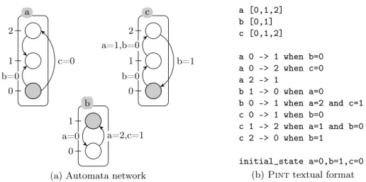
Fig.1 shows an example of automata networks with its plain text
represen-tation in Pint format. By convention, the file names end with .an.
Automata networks are expressive enough to encode the asynchronous se-mantics of Boolean and multi-valued networks. The main difference with these latter frameworks is the explicit specification of local transitions for each au-tomaton (node) of the network, compared to a function-centred specification for
Boolean and multi-valued networks [7,19].
Pint can automatically convert models expressed as Boolean or multi-valued networks using the pint-import command or pypint.load() python function.
Most of the conversions are performed using GINsim [10], enabling the support
for SBML-qual, GINsim, as well as various text formats. Models can be directly
imported from URLs and from CellCollective database [13]. Biocham reaction
networks are also supported, following their Boolean semantics [4].
1
a 0 1 2 c 0 1 2 b 0 1 b=0 c=0 b=0 a=1,b=0 b=1 a=2,c=1 a=0
(a) Automata network
a [0,1,2] b [0,1] c [0,1,2] a 0 -> 1 when b=0 a 0 -> 2 when c=0 a 2 -> 1 b 1 -> 0 when a=0
b 0 -> 1 when a=2 and c=1 c 0 -> 1 when b=0
c 1 -> 2 when a=1 and b=0 c 2 -> 0 when b=1
initial_state a=0,b=1,c=0 (b) Pint textual format
Fig. 1: (a) graphical representation of an automata network: automata are la-belled boxes and their local states by circles where ticks are their identifier within the automaton. The initial state is composed of the local states in gray. A local transition is a directed edge between two local states of an automaton. Transitions can be labelled with states of other automata which are necessary to trigger the transition. (b) equivalent Pint plain text representation
3
Main features and benchmarks
The main originality of Pint resides in the static analysis for transient reacha-bility properties: such an approach avoids building the reachable state transition graph, neither explicitly nor symbolically. Therefore, the analysis aims at being tractable on large networks, at the price of giving possibly incomplete results.
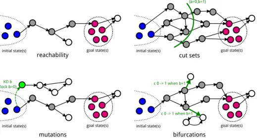
We present the related features, illustrated in Fig. 2, with benchmarks to
support their tractability on large biological networks. Computation times have
been obtained on an Intel CoreR TM i7-4770 3.40GHz CPU with 16GiB RAM.
Reachability analysis: formal approximation and model reduction — Given an initial state, a usual problem is to determine the existence of a se-quence of transitions which leads to the activation or de-activation of key com-ponents (e.g., transcription factors) or to a particular attractor. Reachability verification is a PSPACE-complete problem and its resolution often explodes on large networks. Pint implements over- and under-approximation of reachability
[21,9] which allow tackling large models, although being potentially inconclusive
when the over-approximation is satisfied but not the under-approximation. In such cases, one should fall back to classical model-checking. To that aim, the
goal-oriented reduction [19] identifies transitions that do not contribute to the
goal reachability, and hence can be removed prior to the reachability analysis. This model reduction preserves all minimal traces to the goal, and can enhance
Verification of goal reachability Model (|nodes|) |T| |states| NuSMV (EF g) ITS-reach Pint TCell-d (101) [1] 381 ≈ 2.4 · 108 2s 40Mb 0.5s 26Mb 0.02s profile 1 0 1 TCell-d (101) 381 KO KO 960s 1.6Gb 4.5s profile 2 221 75,947,684 470s 270Mb 15s 160Mb RBE2F (370) [22] 742 KO KO KO 0.2s 56 2,350,494 3s 37Mb 4s 13Mb MAPK (309) [24] 1251 KO KO KO 48s 429 KO KO KO
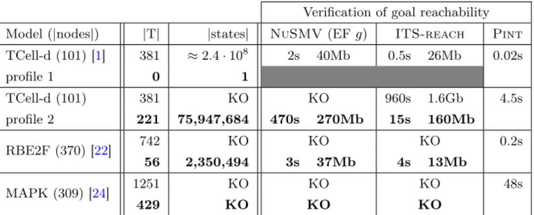
Table 1: Benchmark† of goal reachability verification with two exact methods
(NuSMV and ITS-reach) and Pint, before (normal font) and after (bold font) goal-oriented model reduction; |T| is the number of local transitions in automata networks; |state| is the number of reachable global states, when computable. KO indicates an out-of-memory/time computation. In all cases Pint is conclusive.
TCell-d (101) Egf-r (104) [23] MAPK (309) PID (10,229) [20] Goal FOXP3=1 AP1=1 ERK-PP=1 SNAIL=1 3-cut sets 0.06s 35 0.02s 34 0.06s 24 1.2s 7 4-cut sets 0.10s 101 0.02s 34 0.1s 48 5s 37 6-cut sets 0.60s 495 0.03s 34 1s 60 10m 907 3-mutations 0.30s 15 0.30s 20 5s 222 50m 7 4-mutations 0.30s 15 0.30s 22 10s 1896 50m 67 6-mutations 0.30s 15 0.30s 22 KO 50m 367
Table 2: Performance† of cut sets and mutations under-approximations with
Pint depending on the maximal cardinality of returned sets.
|T| |states| goal NuSMV Pint |tb| time |tb| time
EGF/TNF (28) [17] 53 3968 NFkB = 0 5 0.2s 2 0.1s MAPK (53) [11] 173 KO Proliferation = 1 KO 13 40s TCell-d (101) 381 KO FOXP3 = 1 KO 4 58s
Table 3: Performance† of exact and approximated identification of bifurcation
transitions with NuSMV and Pint, respectively; |tb| is the number of identified
bifurcation transitions. †
initial state(s) goal state(s) initial state(s) goal state(s)
initial state(s) goal state(s)
reachability cut sets
mutations bifurcations
initial state(s) goal state(s)
{a=0,b=1}
c 0 -> 1 when b=1
c 0 -> 1 when b=1 KO b
(lock b=0)
Fig. 2: Illustration of main features of Pint related to the transient reachability of a set of goal states from (a set of) initial state(s). Circles represent global states of the network and plain arrows dynamical transitions. Gray (resp. white) states are states which are (resp. are not) connected to a goal state.
Prediction of mutations for controlling reachability — Given an initial state and a goal state of interest, Pint provides several methods to control the transient reachability of the goal.
The most scalable approach identifies cut sets of all the paths of transi-tions leading to the goal. A cut sets consists in one or several local states of automata which are necessary for the goal reachability: if one prevents the tran-sitions involving these local states, the goal is disconnected from the initial state.
Pint provides extremely scalable under-approximation of cut sets [20], which is
tractable on Boolean networks with thousands of nodes (Table2). Cut sets can
thus be implemented as mutations which lock automata to its initial local state. An alternative approach relies on a combination of static analysis and SAT solving and allows to directly infer mutations (gain or loss of function) which prevent the goal reachability. Whereas less scalable than cut set computations, it provides in general complementary solutions to cut sets, notably by identifying mutations which modify the initial state of the network.
Identification of bifurcation transitions — Pint implements static analysis
for identifying so-called bifurcation transitions [8] after which the systems loses
the capability to reach a given goal. Bifurcation transitions correspond to local transitions of the automata network which turn out to be important decision steps during differentiation processes. They can be fully identified by model-checking, but the static analysis in Pint allows tackling larger models, at the
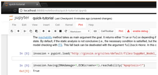
Fig. 3: Screen capture of Jupyter web interface running pypint in a notebook.
4
Integration with Jupyter IPython Web Notebook
Jupyter (http://jupyter.org) provides an interactive web interface for
cre-ating documents, named notebooks, which contain code, equations, and for-matted texts. A notebook typically describes a full workflow of analysis, both with textual explanations and the full code and parameters to reproduce the results. It is a very popular framework in data science, including in
bioinfor-matics [6,12]. A notebook is a single file which can be easily modified, shared,
re-executed, and visualized online. For instance, the companion quick tutorial
is available at http://nbviewer.jupyter.org/github/pauleve/pint/blob/
master/notebook/quick-tutorial.ipynb.
The pypint module provides custom integration within the Jupyter IPython notebook, with custom menus and actions for loading models and executing
Pint commands, as well as direct visualization of data structures. See Fig. 3
and the companion quick tutorial for a preview.
5
Conclusion
In this paper, we presented the prominent features of Pint on the static analysis for transient reachability of automata networks, from property verification to inference, which are tractable on large biological networks. Pint also implements classical state transition graph analysis, from fixpoint computation (using SAT solving) to explicit state space exploration, with a limited scalability. A tour of
features is given at https://loicpauleve.name/pint/doc/#Tutorial.
In the next major release, we plan to add full support for synchronized local transitions, i.e., transitions that modify simultaneously the state of several au-tomata. This improvement will allow to import any safe (1-bounded) Petri nets, broadening the class of supported dynamical models.
References
1. W. Abou-Jaoudé, P. T. Monteiro, A. Naldi, M. Grandclaudon, V. Soumelis, C. Chaouiya, and D. Thieffry. Model checking to assess t-helper cell plasticity. Frontiers in Bioengineering and Biotechnology, 2, Jan 2015.
2. T. Antao. Bioinformatics with Python cookbook. Packt Publishing Ltd, 2015. 3. C. Baral. Knowledge Representation, Reasoning and Declarative Problem Solving.
Cambridge University Press, New York, NY, USA, 2003.
4. L. Calzone, F. Fages, and S. Soliman. Biocham: an environment for model-ing biological systems and formalizmodel-ing experimental knowledge. Bioinformatics, 22(14):1805–1807, 2006.
5. A. Cimatti, E. Clarke, E. Giunchiglia, F. Giunchiglia, M. Pistore, M. Roveri, R. Se-bastiani, and A. Tacchella. NuSMV 2: An opensource tool for symbolic model checking. In Computer Aided Verification, volume 2404 of Lecture Notes in Com-puter Science, pages 241–268. Springer Berlin / Heidelberg, 2002.
6. P. J. A. Cock, T. Antao, J. T. Chang, B. A. Chapman, C. J. Cox, A. Dalke, I. Fried-berg, T. Hamelryck, F. Kauff, B. Wilczynski, and M. J. L. de Hoon. Biopython: freely available python tools for computational molecular biology and bioinformat-ics. Bioinformatics, 25(11):1422–1423, mar 2009.
7. F. Fages, T. Martinez, D. A. Rosenblueth, and S. Soliman. Influence Systems vs Reaction Systems, pages 98–115. Springer International Publishing, Cham, 2016. 8. L. F. Fitime, O. Roux, C. Guziolowski, and L. Paulevé. Identification of
bi-furcations in biological regulatory networks using answer-set programming. In Constraint-Based Methods for Bioinformatics Workshop, 2016.
9. M. Folschette, L. Paulevé, M. Magnin, and O. Roux. Sufficient conditions for reachability in automata networks with priorities. Theoretical Computer Science, 608, Part 1, From Computer Science to Biology and Back:66 – 83, 2015.
10. A. G. Gonzalez, A. Naldi, L. Sánchez, D. Thieffry, and C. Chaouiya. Ginsim: A software suite for the qualitative modelling, simulation and analysis of regulatory networks. Biosystems, 84(2):91 – 100, 2006. Dynamical Modeling of Biological Regulatory Networks.
11. L. Grieco, L. Calzone, I. Bernard-Pierrot, F. Radvanyi, B. Kahn-Perlès, and D. Thi-effry. Integrative modelling of the influence of MAPK network on cancer cell fate decision. PLoS Comput Biol, 9(10):e1003286, oct 2013.
12. R. Grunberg, M. Nilges, and J. Leckner. Biskit — a software platform for structural bioinformatics. Bioinformatics, 23(6):769–770, jan 2007.
13. T. Helikar, B. Kowal, S. McClenathan, M. Bruckner, T. Rowley, A. Madrahimov, B. Wicks, M. Shrestha, K. Limbu, and J. A. Rogers. The cell collective: Toward an open and collaborative approach to systems biology. BMC Systems Biology, 6(1):96, 2012.
14. H. Klarner, A. Streck, and H. Siebert. PyBoolNet: a python package for the generation, analysis and visualization of boolean networks. Bioinformatics, page btw682, oct 2016.
15. F. d. V. Leprevost, B. A. Grüning, S. Alves Aflitos, H. L. Röst, J. Uszkoreit, H. Barsnes, M. Vaudel, P. Moreno, L. Gatto, J. Weber, M. Bai, R. C. Jimenez, T. Sachsenberg, J. Pfeuffer, R. Vera Alvarez, J. Griss, A. I. Nesvizhskii, and Y. Perez-Riverol. Biocontainers: An open-source and community-driven frame-work for software standardization. Bioinformatics (Oxford, England), Mar. 2017. 16. LIP6/Move. Its tools. http://ddd.lip6.fr/itstools.php.
17. A. MacNamara, C. Terfve, D. Henriques, B. P. Bernabé, and J. Saez-Rodriguez. State–time spectrum of signal transduction logic models. Physical Biology, 9(4):045003, 2012.
18. C. Mussel, M. Hopfensitz, and H. A. Kestler. BoolNet – an R package for generation, reconstruction and analysis of boolean networks. Bioinformatics, 26(10):1378–1380, 2010.
19. L. Paulevé. GoalOriented Reduction of Automata Networks. In CMSB 2016 -14th conference on Computational Methods for Systems Biology, volume 9859 of Lecture Notes in Bioinformatics. Springer, 2016.
20. L. Paulevé, G. Andrieux, and H. Koeppl. Under-approximating cut sets for reach-ability in large scale automata networks. In N. Sharygina and H. Veith, editors, Computer Aided Verification, volume 8044 of Lecture Notes in Computer Science, pages 69–84. Springer Berlin Heidelberg, Berlin, Heidelberg, 2013.
21. L. Paulevé, M. Magnin, and O. Roux. Static analysis of biological regulatory net-works dynamics using abstract interpretation. Mathematical Structures in Com-puter Science, 22(04):651–685, 2012.
22. A. Rougny, C. Froidevaux, L. Calzone, and L. Paulevé. Qualitative dynamics semantics for SBGN process description. BMC Systems Biology, 10(1):1–24, 2016. 23. R. Samaga, J. Saez-Rodriguez, L. G. Alexopoulos, P. K. Sorger, and S. Klamt. The logic of egfr/erbb signaling: Theoretical properties and analysis of high-throughput data. PLoS Comput Biol, 5(8):e1000438, 08 2009.
24. B. Schoeberl, C. Eichler-Jonsson, E. D. Gilles, and G. Müller. Computational modeling of the dynamics of the map kinase cascade activated by surface and internalized egf receptors. Nature biotechnology, 20(4):370–375, 2002.