People's Democratic Republic of Algeria
Ministry of Higher Education and Scientific Research
University 08 May 1945 – Guelma-
Faculty of Sciences and Technology
Department of Electrotechnique and Automatic Engineering
A THESIS
Submitted in Partial Fulfillment of the Requirements for the Degree of
DOCTOR of SCIENCES
Title
By Yassine YAKHELEF
Before the jury:
Pr. H. TEBBIKH Prof. at Univ. of 08 May 1945-Guelma President Dr. M. BOULOUH (MCA) S. Lecturer at Univ. of 08 May 1945-Guelma Supervisor Pr. E. HADJADJ AOUL Prof. at Univ. of Badji Mokhtar-Annaba Examiner Pr. S. SAAD Prof. at Univ. of Badji Mokhtar-Annaba Examiner
GUELMA 2015
Parametric Optimization of PI Speed Regulators and
State Observer based Control Systems with Viscous
Friction Coefficient Account using Mini-Max Approach
République Algérienne Démocratique et Populaire
Ministère de l’Enseignement Supérieur et de la Recherche Scientifique
Université 08 Mai 1945- Guelma
Faculté des Sciences et de la Technologie
Département de Génie Electrotechnique et Automatique
THÈSE
Présentée pour l’Obtention du Grade de
DOCTEUR en SCIENCES
:
Titre
Par: Yassine YAKHELEF Jury:
Dr., Prof. H.TEBBIKH Université 08 Mai 1945 Guelma Président Dr., M.C.A M. BOULOUH Université 08 Mai 1945 Guelma Rapporteur
Dr., Pr. E. HADJADJ AOUL Université Badji Mokhtar Annaba Examinateur Dr., Pr. S. SAAD Université Badji Mokhtar Annaba Examinateur
GUELMA 2015
Optimisation Paramétrique des Systèmes de Commande à
Régulateurs PI et Observateur d’Etat sous l’Influence de
Parametric Optimization of PI Speed Regulators and State
Observer based Control Systems with Viscous Friction Coefficient
Account using Mini-Max Approach
A thesis submitted for the degree of
Doctor of Sciences
By
Yassine Yakhelef
Department of Electrotechnics and Automatic Engineering Faculty of Sciences and Technology
University of 08 May 1945 of Guelma 2015
i
Acknowledgements
This thesis was written during my Doctoral studies at the department of Electrotechnique and Automatic Engineering at University of 8 May 1945- Guelma, Faculty of Engineering Sciences and Technology. For this:
First of all, I would like to express my deepest gratitude to my supervisor Dr. Boulouh Messaoud for his guidance, support and motivation during the achievement of this work.
My sincere and deep gratitude is due to Pr. Tebbikh Hicham, Pr. Hadjadj Aoul Elias and Pr. Saad Salah for their acceptance to evaluate this work.
I have to express my grateful thanks to the president of Laboratory of Automatics and Informatics of Guelma (L.A.I.G) and all the members of the Lab., for giving me the opportunity to discuss the most parts of this work during the organized days of JSS, grateful thanks go to them for their many comments and valuable discussions.
I cannot forget to thank the staff of Electrotechnique and Automatic Engineering Department for their kindness.
Yakhele Yassine 2015.
ii
Abstract
The need to improve the quality and performance of electromechanical drive control systems is crucial, where the objective is to increase the production quality of industrial processes and to use rationally our resources. In order to attain this aim, it is necessary to improve and perfecting all quality performance indices of these systems and maintaining them at the required level.
Separately excited DC drive speed control systems, especially those used in rolling mill industries, are characterized by joint elasticity and some aspects of non linearity. This is mainly due to the long shaft coupling the driving motor and the load, which causes substantial torsional vibration in case of load side parameters variation of speed and /or torque changes. These inherent properties can greatly affect the quality of the rolling material and even influence the stability of the used closed loop control system.
In case of minor changes of these parameters, their influence on drive dynamic behavior may be satisfactorily compensated using conventional speed control algorithms, such as PI controller, and ensuring the required quality and accuracy performance of the system response. However, the effects of substantial parameter changes and variations, which is generally the case for this type of application, can no longer be effectively compensated by these algorithms and it is not possible to obtain satisfactory performance by applying only standard and conventional PI controllers. Therefore, looking for control methods and techniques capable of solving the problem of these applications’ drives and achieving improvement of their performances is crucial. In this vein, our work consists of applying the proposed Mini-Max optimization approach in conjunction with other compensation techniques on chosen system models to improve and perfecting the performances of an already existing PI speed controller based separately excited DC drive system and increasing thereafter its
iii
order of astatism under variable operational conditions of set point speed change and load torque disturbance.
On the other hand, these drives are also equipped with current limiter to protect against any damage of the drive components when abrupt set point change or load torque disturbance occur. Unfortunately, the presence of these devices may lead, under those conditions, to saturation of PI speed controller output and consequent serious degradation in system performance is evident. Therefore, the effect of inherent actuator saturation (non-linearity) on degrading the drive’s transient and steady-state performances is also studied, where the effectiveness and efficiency of the proposed novel conditional integration anti-windup compensation technique is verified for this purpose.
Key words: Mini-max Optimisation Approach, Double PI Speed Controller, State Observer, Order of Astatism, Anti Wind up, Saturation, Control Performance Quality.
iv
Résumé
“Optimisation Paramétrique des Systèmes de Commande Electrique à Régulateurs PI et Observateurs d’Etat sous l’Influence de la Friction Visqueuse, par l’Approche
Minimax”
Le problème du perfectionnement des équipements et des technologies dans le but d’améliorer la qualité de production et d’augmenter la productivité et l’utilisation rationnelle des ressources est l’une des priorités primordiales en industrie. Sa résolution est impossible sans l’amélioration progressive de tous les indices de performance de la qualité de commande des systèmes électromécaniques et des processus industriels et leur maintien au niveau requis.
Les systèmes électromécaniques d’entrainement à base des moteurs à courant continu sont largement utilisés dans, particulièrement, les laminoirs industriels pour les métaux, les laminoirs à papier, à verre …etc. Dans ces industries, ce système de commande en vitesse est caractérisé par son élasticité avec quelques aspects non linéaires dûs principalement à la longueur de l’arbre liant le moteur d’entrainement avec la charge mécanique. A cet effet, des vibrations prennent naissance pendant le fonctionnement sous la présence d’une variation ou changement des paramètres extérieurs de vitesse de consigne et/ou du couple de la charge. Ces conditions de fonctionnement ont certainement une influence sur la qualité du produit ainsi que les performances du système de commande utilisé.
Dans le cas où ces variations paramétriques sont légères, leur influence sur le comportement dynamique du système peut, d’une manière satisfaisante, être compensée par les algorithmes de commande conventionnels tels que le correcteur PI. Mais cette compensation devient insuffisante, lorsque ces variations de vitesse ou du couple de la charge sont importantes, ce qui peut nuire aux performances du système.
v
Par conséquence, les chercheurs dans ce domaine, ont pu développer des méthodes et des techniques capables de résoudre ce problème de commande et améliorer ainsi les performances de ces systèmes, ce qui représente une issue primordiale pour le développement technologique.
Ce travail s’insère dans le cadre de l’exploitation rationnelle des ressources matérielles des industries, des différents types de systèmes de régulation de vitesse en cascade à courant continu, utilisant des régulateurs PI ou PID, où on a proposé d’optimiser les paramètres de ses régulateurs par l’approche MiniMax, en la comparant avec d’autres techniques de perfectionnement, sur des modèles choisis, en vue de réaliser une amélioration et un perfectionnement des performances et augmenter l’ordre d’astatisme de ces systèmes durant leur fonctionnement selon les conditions de variation ou changement de la vitesse de consigne et le couple de la charge.
Par ailleurs, une étude approfondie lié au problème de la stabilité en présence de la limitation en courant par la non linéarité “saturation” a été exposée. Cette limitation, précédemment introduite, conduit à un comportement non linéaire, lorsque la boucle de courant se sature, en fort signal pour le cas d’un système à un seul correcteur PI et en faible signal pour le cas d’un correcteur PI double, ce qui provoque l’apparition de fortes oscillations, voire des cycles limites instables. Pour pallier à ce problème d’instabilité, une solution a été proposée sous forme de schémas de structure et de principe, qui peut être utilisée en cas de limitation en courant pour la classe des systèmes de régulation de vitesse en cascade avec un nombre d’intégrateurs variable, assurant ainsi une stabilité et une qualité de commande optimale.
Mots clés: Approche Minimax, Régulateur de Vitesse PI, Observateur d’État, Ordre d’Astatism, Saturation, performance et qualité de commande.
vi
نإ ما ا ةء او ا ةد زو ج ا ةد او تا "# ا $ %& ' () *ا + , ا ت وأ ) ة .او ھ + , ا درا # ا . 1 #2 2 ر ا ا ) 34 ف 6 ا ا7ھ 8 9 ب '%# ا ى # ا <'+ ظ او + , ا ت '#" او )و$6 ا #> *ا ?@ا$) ءاد*ا ةد تا$AB) . ت C$ # ا س أ <'+ )و$6 ا '#. E> 1 او ق % <'+ م &و ر ا تاذ $# # ا H (3 ، %# ا ،ص K ج L او قر ا 1 ,) ،ند "#' + , ا . ... E ا م > L # و ،ت + , ا ه7ھ N ا صا$@أ ك$ ) P3ر Q)ر ل ط < إ أ % ا $ T 9 # ا U ا V"3 1) W و$) لXK ) Y ذ +$ # ا H# ا 1) . فX Kا د و H Z( ا ء [أ تازاL ھ4ا \( & ،ض$Z ا ا76 ر ا E "# ا $ Z& وأ و +$ P?^ / ءU" ا ا7ھ ) نارو ا مL+ وأ . + X_ ،ج # ا ةد <'+ $ [\& C\ 3 6 فو$> ا ه7ھ ) # ا E ا م > ءادأ . ت )زرا K 6^ " نأ # م > ' ) ا ك ' ا <'+ ھ$ [\&و ،ة$ Z` ت X K4ا ه7ھ . 8@ # ا Ha) '9 ا E ا ? & -') & , +$ ت X K4ا ه7ھ + ف C $ T Q?, V " ا ا7ھ م > ا ءاد\3 H & نأ # او ،E6) $)أ H# ا ) نارو ا مL+ وأ . ،ل 2# ا ا7ھ b ? ا ن ،Y 7 2 و ه7ھ ) HC () H. <'+ ةرد @ ت 9&و U أ $ %&و أ \ ) " ، #> *ا ه7ھ ءادأ و ا ر % ا . E ا #> أ ) ' ) عا أو ، د # ا درا # ا ت + ,' A$ ا ما 4ا ) اءL ھ H#" ا ا7ھ ما 3 Y ذو ،ك$ # ا & +$ E> ) +$ ? & -') & وأ ? & -') & -8 () ، ح$ 9 b . لXK ) #> # ا تادا +إ 9 $ط ‘ eC # ) ’ ،ةر ) ى$K*ا جذ # و ت 9 ا 1) Y ذ ر 9)و ، ةد زو ءاد*ا $ %&و & 8 9 رد را$9 4ا $ Z ا وأ فX K4ا فو$ظ Hظ E> ا ه76 H# ا نارود مL+و ةد # ا +$ ا . ةوX+و د @ د و را$9 4ا ' (#3 8'" & ') A ار b ? ا ا7ھ ض$" ا E& 9 ،Y ذ <'+
%KX ا H?@ ) ا " 1?( ا ". 9'. 1?( ) + % ا $ T ك ' < إ يدB #) ، 93 م @ ، 9 ا ا7ھ Q ,& 1) م > . @ ةر Aإ ا ? & -') & ةر Aإو .او Q ,) د و . "^ ? & -') & ة$9 ) $ T . تارود وأ @ تازاL ھا ر 6ظ U? ي7 او ،جودL# ا . ه7ھ <'+ U'Z ' g ا 9 ا . 6)ا ا # او ،أ ?# ا b . ) ? ا م $ او H 6C X. ح$ @ا 9 ، ' (# ا ةL6 أ E ا #> أ +$ ا ةد 2 ا ?@ا$)و را$9 4ا ن #^ 3و ،$ Z ) H) & ) د + 1) د$% ا <'a# ا . ح ا ت : 9 $ط eC # ) , رد را$9 4ا , E> ) ? & +$ -') & , ا U@ا$) , 1?( ا , ءاد*ا و ةد 2 ا P?^ .
Contents
Acknowledgements i
Abstract ii
Résumé iv
vi
List of Figures vii
List of Tables xxi
Nomenclature xxiv
1 Introduction 1
1.1 Motivation and Background ……….…..1
1.2 Scope and Objectives of the Thesis ………...8
1.3 Contributions ………..9
1.4 Thesis Structure ………....10
2 Description of Separately Excited DC Drive Control System 12
2.1 Introduction ………...12
2.2 Dynamic Model of Separately Excited DC Motor ………...12
2.2.1 Electrical Characteristics of SEDC Motor ………15
2.2.2 Mechanical Characteristics of SEDC Motor ……….16
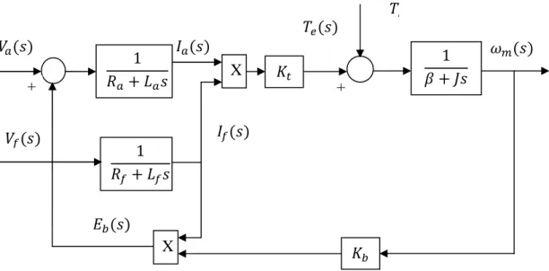
2.3 Block Diagram Representation of SEDC Motor based Electromechanical System ………...17
2.3.1 Suitable Block Diagram Representation ……….. ………18
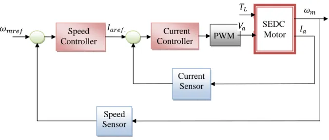
2.5 Speed Control Structures of SEDC Motor ...………...21
2.5.1 Open Loop Speed Control of DC Motor ………...22
2.5.2 Closed Loop Speed Control of DC Motor ………...22
2.5.2.1 Current Controller in DC Drive System ………...23
2.5.3 Speed Controller Selection for SEDC Drive System ………...24
2.5.4 Implementation Forms of PID Controller ……….24
2.5.4.1 Standard Non Interacting Form ……….25
2.5.4.2 Parallel Non Interacting Form ………...25
2.5.4.3 Series Interacting Form ………...26
2.5.5 PI versus PID Utilization in DC Drive Control Systems ………..28
2.6 State Observer Based Feedback Speed Control of DC Drive ………...28
2.7 Elaborated PI based Speed Controlled DC Drive Models for Performance Improvement ………31
2.7.1 System Model with 1PI Speed Controller and State Observer of order 2………31
2.7.2 System Model with 2PI Speed Controller and State Observer of order 2 ...32
2.7.3 System Model with 1PI Speed Controller and State Observer of order 5 ...33
2.7.4 System Model with 2PI Speed Controller and State Observer of order 6 ...34
2.8 Conclusion ………...35
3 DC Drive Dynamic Performance Optimization using Mini-Max Approach 36
3.1 Introduction ………36
3.2 Dynamic Performance Properties of PI Speed Controlled DC Drive …………..36
3.3 Stability vs. Overshoot Performance Properties ………...38
3.4 Dynamic Performance Improvement by Tuning PI Parameters ………40
3.5 Tuning Methods for PID Controller ……….42
3.5.1 Plant Features based Tuning Methods ………...42
3.5.1.1 Zeigler and Nichols tuning methods ………...42
3.5.1.2 Cohen-Coon Tuning Method ………...44
3.5.1.3 Relay Feedback Tuning Method ………45
3.5.2 Analytical Tuning Methods ………...47
3.5.2.1 Pole Placement Tuning Method ………47
3.5.2.2 Dominant Pole Placement Tuning Method ….………...48
3.5.2.3 Internal Mode Control (IMC) Tuning Method ………...49
3.5.3 Optimization based Tuning Methods ……….51
3.5.3.1 Iterative Feedback Tuning (IFT) method ……….51
3.5.3.2 Integral based Minimization Criteria Tuning Method ………53
3.6 Tuning PI Parameters using Mini-Max Optimization Approach ……….56
3.6.1 Simulation Results of Dynamic Performance Improvement ………...57
3.6.1.1 System Model with 1PI Speed Controller and State Observer of order 2…………..58
3.6.1.2 System Model with 2PI Speed Controller and State Observer of order 2 ...62
3.6.1.3 System Model with 1PI Speed Controller and State Observer of order 5...65
3.6.1.4 System Model with 2PI Speed Controller and State Observer of order 6...68
3.7 Results Interpretation and Discussion ……….71
3.8 Conclusion ………72
4 Improving Accuracy Performance and order of Astatism of DC Drive using Feed-Forward Compensation 73
4.2 Preliminaries ……….74
4.2.1 Typical Standard Signals for Accuracy Analysis ………..74
4.2.1.1 Step Function Signal ………...75
4.2.1.2 Ramp Function Signal ………...76
4.2.1.3 Parabolic Function Signal ………...76
4.3 System’s Accuracy Performance Assessment for Variable Set Point …………..77
4.3.1 Calculation of System’s Steady State Error ………..78
4.3.2 Relationship between System Accuracy and its order of Astatism …………81
4.3.3 Simulation Results ……….83
4.3.3.1 System Model with 1PI Speed Controller and State Observer of order 2 ...83
4.3.3.2 System Model with 2PI Speed Controller and State Observer of order 2 …………...84
4.3.3.3 System Model with 1PI Speed Controller and State Observer of order 5 …………...84
4.3.3.4 System Model with 2PI Speed Controller and State Observer of order 6 …………...85
4.3.4 Results Interpretation and Discussion …..……… …..85
4.4 Accuracy Performance Improvement using Feed-Forward Compensation …….86
4.4.1 Previous Work ………...86
4.4.2 Application Feed-Forward Compensation Technique….……...… ……….. ...87
4.4.2.1 System Model with 1PI Speed Controller and State Observer of order 2 …………...89
4.4.2.2 System Model with 2PI Speed Controller and State Observer of order 2 …………...90
4.4.2.3 System Model with 1PI Speed Controller and State Observer of order 5 …………...90
4.4.2.4 System Model with 2PI Speed Controller and State Observer of order 6 …………...91
4.4.3 Results Interpretation and Discussion ………...91
4.5 Improving System’s Accuracy under Load Disturbance Effect ………...91
4.5.2 Simulation Results of Steady State Error under Load Disturbance ...95
4.5.2.1 System Model with 1PI Speed Controller and State Observer of order 2 …………...96
4.5.2.2 System Model with 2PI Speed Controller and State Observer of order 2 …………...96
4.5.2.3 System Model with 1PI Speed Controller and State Observer of order 5 …………...97
4.5.2.4 System Model with 2PI Speed Controller and State Observer of order 6 …………...97
4.5.3 Results Interpretation and Discussion ………...98
4.5.4 Load Torque Disturbance Suppression using Feed-Forward Compensation …………..98
4.5.4.1 System Model with 1PI Speed Controller and State Observer of order 2 …………...99
4.5.4.2 System Model with 2PI Speed Controller and State Observer of order 2 …………...99
4.5.4.3 System Model with 1PI Speed Controller and State Observer of order 5 ………….100
4.5.4.4 System Model with 2PI Speed Controller and State Observer of order 6 ………….100
4.5.5 Results Interpretation and Discussion ……….101
4.6 Conclusion ………...101
5 Study of Nonlinearity and Parameters Variation Effects on System Performance 102 5.1 Introduction ………102
5.2 Drive Systems with Input Saturation Nonlinearities ………..102
5.3 Simulation Results of Actuator Saturation Effects ……….103
5.3.1 System Model with 1PI Speed Controller and State Observer of order 2 ...104
5.3.2 System Model with 2PI Speed Controller and State Observer of order 2 ...105
5.3.3 System Model with 1PI Speed Controller and State Observer of order 5 ...107
5.3.4 System Model with 2PI Speed Controller and State Observer of order 6 ...108
5.3.5 Results Interpretation and Discussion ……….110
5.4 DC Drive Performance Improvement by Saturation Compensation …………..110
5.4.1 Saturation Compensation Techniques ………...110
5.4.1.2 Tracking Back Calculation Anti-Windup Techniques ………...112
5.4.1.3 Conditional Integration Anti-Windup Compensation Techniques ………...113
5.4.2 Novel Conditional Integration Anti-Windup Compensation ………..114
5.4.3 Simulation Results of Actuator Saturation Compensation ………116
5.4.3.1 System Model with 1PI Speed Controller and State Observer of order 2 ……...117
5.4.3.2 System Model with 2PI Speed Controller and State Observer of order 2 ……...118
5.4.3.3 System Model with 1PI Speed Controller and State Observer of order 5 ……...120
5.4.3.4 System Model with 2PI Speed Controller and State Observer of order 6 ……...121
5.4.4 Results Interpretation and Discussion ………...123
5.5 Study of Drive Performance Sensitivity to Parameters Variation ………..123
5.5.1 Simulation Results ………...124
5.5.1.1 System Model with 1PI Speed Controller and State Observer of order 2 ……...124
5.5.1.2 System Model with 2PI Speed Controller and State Observer of order 2 ……...125
5.5.1.3 System Model with 1PI Speed Controller and State Observer of order 5 ……...125
5.5.1.4 System Model with 2PI Speed Controller and State Observer of order 6 ……...126
5.5.2 Results Interpretation and Discussion ………...126
5.6 Conclusion ………..127
General Conclusions and Perspectives 128
Appendices 131
vii
List of Figures
Figure 2.1 Equivalent Circuit of Separately Excited DC Motor based Electromech- -anical System ……….………...…....13 Figure 2.2 Block Diagram of SEDC Motor based Electromechanical System under Variation of both Field and Armature Currents……….………..18 Figure 2.3 Combined Armature Voltage and Field Flux Speed Control of Separately Excited DC Motor………...19 Figure 2.4 Block Diagram of SEDC Motor Electromechanical System under Armature Voltage Control only ………..20 Figure 2.5 Cascade Structure of SEDC Motor Feedback Speed Control Loop………23 Figure 2.6 Interacting and Non- Interacting Forms of PID Controller...27
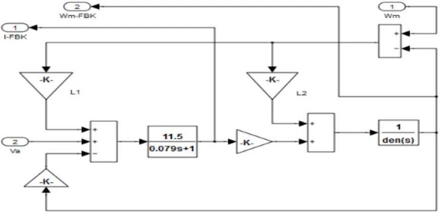
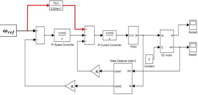
Figure 2.7 General Structure of State Observer based Control System of DC Motor..30 Figure 2.8 Simulink Block Diagram of Model with 1PI Speed Controller and 2nd order
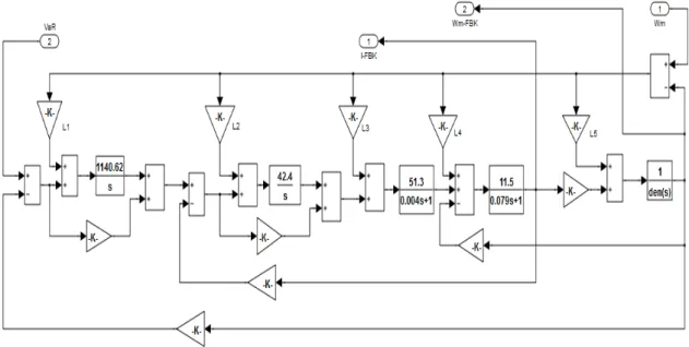
State Observer based DC Drive System………. ………32 Figure 2.9 Simulink Block Diagram of 2nd order State Observer Structure…………..32 Figure 2.10 Simulink Block Diagram of Model with 2PI Speed Controller and 2nd order State Observer based DC Drive System………..32 Figure 2.11 Simulink Block Diagram Model of one PI Speed Controller and 5th order State Observer based DC Drive System………33 Figure 2.12 Simulink Block Diagram of 5th order State Observer Structure…………33 Figure 2.13 Simulink Block Diagram Model of 2PI Speed Controller and 6th order State Observer based DC Drive System……….34 Figure 2.14 Simulink Block Diagram of 6th order State Observer Structure…………34 Figure 3.1 Typical Step Response of DC Drive Control System………38 Figure 3.2 Percent Overshoot and Phase Margin as a Function of Damping Ratio ξ.40 Figure 3.3 Block Diagram of Relay Feedback Tuning Method ……….46 Figure 3.4 Pole-Zero Configuration of a Simple Feedback System used by Dominant
viii
Figure 3.5 Internal Model Control Structure Block Diagram for PID Tuning………..50 Figure 3.6 Block Diagram Illustrating IFT Method for PID Tuning...……….52 Figure 3.7 Variation of Tracking Error Function with respect to PI Parameter Vector and Time. ………57 Figure 3.8 Responses as Optimized with Mini-Max, I.A.E., I.S.E., I.T.A.E. and Compared to not Optimized Response for the Model with 1PI Speed Controller, State Observer of order 2 and = ; a) Output Speed, b) Tracking Speed Error...58 Figure 3.9 Responses as Optimized with Mini-Max, I.A.E., I.S.E., I.T.A.E. and Compared to not Optimized Response for the Model with 1PI Speed Controller, State Observer of order 2 and > 0; a) Output Speed, b) Tracking Speed Error...59 Figure 3.10 Responses as Optimized with Mini-Max, I.A.E., I.S.E., I.T.A.E. and Compared to not Optimized Response for the Model with 1PI Speed Controller, State Observer of order 2 and < 0; a) Output Speed, b) Tracking Speed Error...59 Figure 3.11 Responses showing the Effect of when Optimized with Mini-Max for the Model with 1PI Speed Controller and State Observer of order 2; a) Output Speed, b) Tracking Speed Error...60 Figure 3.12 Responses as Optimized with Mini-Max, I.A.E., I.S.E., I.T.A.E. and Compared to not Optimized Response for the Model with 2PI Speed Controller, State Observer of order 2 and = ; a) Output Speed, b) Tracking Speed Error...62 Figure 3.13 Responses as Optimized with Mini-Max, I.A.E., I.S.E., I.T.A.E. and Compared to not Optimized Response for the Model with 2PI Speed Controller, State Observer of order 2 and > 0; a) Output Speed, b) Tracking Speed Error...62 Figure 3.14 Responses as Optimized with Mini-Max, I.A.E., I.S.E., I.T.A.E. and Compared to not Optimized Response for the Model with 2PI Speed Controller, State Observer of order 2 and < 0; a) Output Speed, b) Tracking Speed Error...63 Figure 3.15 Responses showing the Effect of when Optimized with Mini-Max for the Model with 2PI Speed Controller and State Observer of order 2; a) Output Speed,
b) Tracking Speed Error...63 Figure 3.16 Responses as Optimized with Mini-Max, I.A.E., I.S.E., I.T.A.E. and Compared to not Optimized Response for the Model with 1PI Speed Controller, State Observer of order 5 and = ; a) Output Speed, b) Tracking Speed Error...65
Figure 3.17 Responses as Optimized with Mini-Max, I.A.E., I.S.E., I.T.A.E. and Compared to not Optimized Response for the Model with 1PI Speed Controller, State Observer
ix
of order 5 and > 0; a) Output Speed, b) Tracking Speed Error...65 Figure 3.18 Responses as Optimized with Mini-Max, I.A.E., I.S.E., I.T.A.E. and Compared to not Optimized Response for the Model with 1PI Speed Controller, State Observer of order 5 and < 0; a) Output Speed, b) Tracking Speed Error...66 Figure 3.19 Responses showing the effect of when optimized with Mini-Max for the Model with 1PI Speed Controller and State Observer of order 5; a) Output Speed, b)
Speed Tracking Error...66 Figure 3.20 Responses as Optimized with Mini-Max, I.A.E., I.S.E., I.T.A.E. and Compared to not Optimized Response for the Model with 2PI Speed Controller, State Observer of order 6 and = ; a) Output Speed, b) Tracking Speed Error... ....68 Figure 3.21 Responses as Optimized with Mini-Max, I.A.E., I.S.E., I.T.A.E. and Compared to not Optimized Response for the Model with 2PI Speed Controller, State Observer of order 6 and > 0; a) Output Speed, b) Tracking Speed Error...68 Figure 3.22 Responses as Optimized with Mini-Max, I.A.E., I.S.E., I.T.A.E. and Compared to not Optimized Response for the Model with 1PI Speed Controller, State Observer
of order 5 and < 0; a) Output Speed, b) Tracking Speed Error...69 Figure 3.23 Responses showing the effect of when optimized with Mini-Max for the Model with 1PI Speed Controller and State Observer of order 5; a) Output Speed, b)
Speed Tracking Error...69 Figure 4.1 General Block Diagram of DC Drive Control System without Load
Disturbance Signal………...77 Figure 4.2 Speed Tracking Error Response of System Model with 1PI Speed
Controller and State Observer of order 2 due to Input Set Point Changes; a) case of = 0, b) case of > 0, c) case of < 0………..83 Figure 4.3 Speed Tracking Error Response of System Model with 2PI Speed
Controller and State Observer of order 2 due to Input Set Point Changes; a) case of = 0, b) case of > 0, c) case of < 0………..84 Figure 4.4 Speed Tracking Error Response of System Model with 1PI Speed
Controller and State Observer of order 5 due to Input Set Point Changes; a) case of = 0, b) case of > 0, c) case of < 0……….84 Figure 4.5 Speed Tracking Error Response of System Model with 2PI Speed
x
case of = 0, b) case of > 0, c) case of < 0………..85 Figure 4.6 Typical Block Diagram of System Model with 1PI and State Observer of order 2 Incorporating Feed-Forward Compensation Technique………….88 Figure 4.7 Steady State Error and order of Astatism Improvement with Feed-Forward Compensation of System Model with 1PI and State Observer of order 2 under Input Set Point Changes; a) case of = 0, b) case of > 0, c) case of < 0………89 Figure 4.8 Steady State Error and order of Astatism Improvement with Feed-Forward Compensation of System Model with 2PI and State Observer of order 2 under Input Set Point Changes; a) case of = 0, b) case of > 0, c) case of < 0………...90 Figure 4.9 Steady State Error and order of Astatism Improvement with Feed-Forward Compensation of System Model with 1PI and State Observer of order 5 under Input Set Point Changes; a) case of = 0, b) case of > 0, c) case of < 0………90 Figure 4.10 Steady State Error and order of Astatism Improvement with Feed-Forward Compensation of System Model with 2PI and State Observer of order 6 under Input Set Point Changes; a) case of = 0, b) case of > 0, c) case of < 0……….91 Figure 4.11 General Block Diagram of DC Drive Control System with Load
Disturbance Signal Account………..92 Figure 4.12 Equivalent Block Diagram of DC Drive System under the Independent
effect of Set Point (a) and Load Disturbance (b) Variations ………….93 Figure 4.13 Speed Tracking Error Response of System Model with 1PI Speed
Controller and State Observer of order 2 due to Load Torque Disturbance; a) case of = 0, b) case of > 0, c) case of < 0………...96 Figure 4.14 Speed Tracking Error Response of System Model with 2PI Speed
Controller and State Observer of order 2 due to Load Torque Disturbance; a) case of = 0, b) case of > 0, c) case of < 0………..96 Figure 4.15 Speed Tracking Error Response of System Model with 1PI Speed
xi
a) case of = 0, b) case of > 0, c) case of < 0………..97 Figure 4.16 Speed Tracking Error Response of System Model with 2PI Speed
Controller and State Observer of order 6 due to Load Torque Disturbance; a) case of = 0, b) case of > 0, c) case of < 0………..97 Figure 4.17 Typical Block Diagram of System Model with 1PI and State Observer of order 2 Incorporating Feed-Forward Load Torque Disturbance
Compensation………98 Figure 4.18 Steady State Error Improvement with Feed-Forward Compensation of System Model with 1PI and State Observer of order 2 under Load Torque Disturbance; a) case of = 0, b) case of > 0, c) case of < 0……..99 Figure 4.19 Steady State Error Improvement with Feed-Forward Compensation of System Model with 2PI and State Observer of order 2 under Load Torque Disturbance; a) case of = 0, b) case of > 0, c) case of < 0……..99 Figure 4.20 Steady State Error Improvement with Feed-Forward Compensation of System Model with 1PI and State Observer of order 5 under Load Torque
Disturbance; a) case of = 0, b) case of > 0, c) case of < 0…….100 Figure 4.21 Steady State Error Improvement with Feed-Forward Compensation of System Model with 2PI and State Observer of order 6 under Load Torque
Disturbance; a) case of = 0, b) case of > 0, c) case of < 0……100 Figure 5.1 Typical Actuator Saturation Characteristic………103 Figure 5.2 Speed response of System Model with 1PI, State Observer of order 2 and = 0 in Presence of Actuator Saturation: a) using speed set point value: 8.2V and b) using speed set point value: 10 V………..104 Figure 5.3 Speed Response of System Model with 1PI, State Observer of order 2 and > 0 in Presence of Actuator Saturation: a) using speed set point value: 8.2V and b) using speed set point value: 10 V………..104 Figure 5.4 Speed Response of System Model with 1PI, State Observer of order 2 and < 0 in Presence of Actuator Saturation: a) using speed set point value: 8.2V and b) using speed set point value: 10 V………. …105 Figure 5.5 Speed Response of System Model with 2PI, State Observer of order 2 and = 0 in Presence of Actuator Saturation: a) using speed set point value:
xii
8.2V and b) using speed set point value: 10 V………..105 Figure 5.6 Speed Response of System Model with 2PI, State Observer of order 2 and > 0 in Presence of Actuator Saturation: a) using speed set point value: 8.2V and b) using speed set point value: 10 V………..106 Figure 5.7 Speed Response of System Model with 2PI, State Observer of order 2 and < 0 in Presence of Actuator Saturation: a) using speed set point value: 8.2V and b) using speed set point value: 10 V………..106 Figure 5.8 Speed Response of System Model with 1PI, State Observer of order 5 and = 0 in Presence of Actuator Saturation: a) using speed set point value: 8.2V and b) using speed set point value: 10 V………..107 Figure 5.9 Speed Response of System Model with 1PI, State Observer of order 5 and > 0 in Presence of Actuator Saturation: a) using speed set point value: 8.2V and b) using speed set point value: 10 V………..107 Figure 5.10 Speed Response of System Model with 1PI, State Observer of order 5 and < 0 in Presence of Actuator Saturation: a) using speed set point value: 8.2V and b) using speed set point value: 10 V……….108 Figure 5.11 Speed Response of System Model with 2PI, State Observer of order 6 and = 0 in Presence of Actuator Saturation: a) using speed set point value: 8.2V and b) using speed set point value: 10 V……….108 Figure 5.12 Speed Response of System Model with 2PI, State Observer of order 6 and > 0 in Presence of Actuator Saturation: a) using speed set point value: 8.2V and b) using speed set point value: 10 V……….109 Figure 5.13 Speed Response of System Model with 2PI, State Observer of order 6 and < 0 in Presence of Actuator Saturation: a) using speed set point value: 8.2V and b) using speed set point value: 10 V……….109 Figure 5.14 PI Controller with Dead Zone Limiting Integrator Anti-Windup Scheme… ……….………111 Figure 5.15 PI Controller with Tracking Back Calculation Anti-Windup Scheme…112 Figure 5.16 PI Controller with Conditional Integration Anti-Windup Scheme……..113 Figure 5.17 Block Diagram of Single PI Speed Controller Incorporating the Proposed Conditional Integration Anti-Windup Compensator………...115
xiii
Figure 5.18 Block Diagram of Double PI Speed Controller Incorporating the Proposed Conditional Integration Anti-Windup Compensator………...115 Figure 5.19 Speed Response of System Model with 1PI, State Observer of order 2 and = 0 Incorporating the Novel Conditional Integration Anti-Windup Compensator: a) using Speed Set Point Value: 8.2V and b) using Speed Set Point Value: 10 V………..117 Figure 5.20 Speed Response of System Model with 1PI, State Observer of order 2 and > 0 Incorporating the Novel Conditional Integration Anti-Windup Compensator: a) using Speed Set Point Value: 8.2V and b) using Speed Set Point Value: 10 V ………..117 Figure 5.21 Speed Response of System Model with 1PI, State Observer of order 2 and < 0 Incorporating the Novel Conditional Integration Anti-Windup Compensator: a) using Speed Set Point Value: 8.2V and b) using Speed Set Point Value: 10 V………..118 Figure 5.22 Speed Response of System Model with 2PI, State Observer of order 2 and = 0 Incorporating the Novel Conditional Integration Anti-Windup Compensator: a) using Speed Set Point Value: 8.2V and b) using Speed Set Point Value: 10 V………..118 Figure 5.23 Speed Response of System Model with 2PI, State Observer of order 2 and > 0 Incorporating the Novel Conditional Integration Anti-Windup Compensator: a) using Speed Set Point Value: 8.2V and b) using Speed Set Point Value: 10 V………..119 Figure 5.24 Speed Response of System Model with 2PI, State Observer of order 2 and < 0 Incorporating the Novel Conditional Integration Anti-Windup Compensator: a) using Speed Set Point Value: 8.2V and b) using Speed Set Point Value: 10 V………...119 Figure 5.25 Speed Response of System Model with 1PI, State Observer of order 5 and = 0 Incorporating the Novel Conditional Integration Anti-Windup Compensator: a) using Speed Set Point Value: 8.2V and b) using Speed Set Point Value: 10 V……….120 Figure 5.26 Speed Response of System Model with 1PI, State Observer of order 5 and
xiv
> 0 Incorporating the Novel Conditional Integration Anti-Windup Compensator: a) using Speed Set Point Value: 8.2V and b) using Speed Set Point Value: 10 V………..120 Figure 5.27 Speed Response of System Model with 1PI, State Observer of order 5 and < 0 Incorporating the Novel Conditional Integration Anti-Windup Compensator: a) using Speed Set Point Value: 8.2V and b) using Speed Set Point Value: 10 V………..121 Figure 5.28 Speed Response of System Model with 2PI, State Observer of order 6 and = 0 Incorporating the Novel Conditional Integration Anti-Windup Compensator: a) using Speed Set Point Value: 8.2V and b) using Speed Set Point Value: 10 V………..121 Figure 5.29 Speed Response of System Model with 2PI, State Observer of order 6 and > 0 Incorporating the Novel Conditional Integration Anti-Windup Compensator: a) using Speed Set Point Value: 8.2V and b) using Speed Set Point Value: 10 V……….122 Figure 5.30 Speed Response of System Model with 2PI, State Observer of order 6 and < 0 Incorporating the Novel Conditional Integration Anti-Windup Compensator: a) using Speed Set Point Value: 8.2V and b) using Speed Set Point Value: 10 V………. 122 Figure 5.31 Effect of Drive Parameters Variation on the Optimized Performance of System Model with 1PI Speed Controller and State Observer of order 2: a), c) and e) are Speed Responses under Mini-Max Optimization, b), d) and f) are Responses under Mini-Max Optimization and Saturation
Account………124 Figure 5.32 Effect of Drive Parameters Variation on the Optimized Performance of System Model with 2PI Speed Controller and State Observer of order 2: a), c) and e) are Speed Responses under Mini-Max Optimization, b), d) and f) are Responses under Mini-Max Optimization and Saturation
Account………125 Figure 5.33 Effect of Drive Parameters Variation on the Optimized Performance of System Model with 1PI Speed Controller and State Observer of order 5:
xv
a), c) and e) are Speed Responses under Mini-Max Optimization, b), d) and f) are Responses under Mini-Max Optimization and Saturation
Account………..125 Figure 5.34 Effect of Drive Parameters Variation on the Optimized Performance of System Model with 2PI Speed Controller and State Observer of order 6: a), c) and e) are Speed Responses under Mini-Max Optimization, b), d) and f) are Responses under Mini-Max Optimization and Saturation
Account………126 Figure A.1 Separately Excited DC Motor Equivalent Circuit ………132 Figure A.2 Series DC Motor Schematic Representation ……….132 Figure A.3 Shunt DC motor ………...133 Figure A.4 Compound DC Motor … ………...133
xxi
List of Tables
Table 2.1 Parameters of DC Motor based Electromechanical System………..14 Table 3.1 Effect of changing Independently PID Parameters on System Response….41 Table 3.2 Ziegler-Nichols Formulas for Step Response Tuning Method...43 Table 3.3Ziegler-Nichols Formulas for Frequency Response Tuning Method...44 Table 3.4 Cohen-Coon Controller Tuning Parameters………..45 Table 3.5 Numerical Results of Dynamic Performance Improvement as Optimized with Mini-Max, I.A.E., I.S.E., I.T.A.E. and Compared to not Optimized Response for the Model with 1PI Speed Controller, State Observer of order 2 and = ...60 Table 3.6 Numerical Results of Dynamic Performance Improvement as Optimized with Mini-Max, I.A.E., I.S.E., I.T.A.E. and Compared to not Optimized Response for the Model with 1PI Speed Controller, State Observer of order 2 and > 0...61 Table 3.7 Numerical Results of Dynamic Performance Improvement as Optimized with Mini-Max, I.A.E., I.S.E., I.T.A.E. and Compared to not Optimized Response for the Model with 1PI Speed Controller, State Observer of order 2 and < 0...61 Table 3.8 Numerical Results of Peak Overshoot Improvement as Achieved with Mini- Max Optimization and Affected by the Viscous Friction Coefficient for the Model with 1PI Speed Controller and State Observer of order 2...61 Table 3.9 Numerical Results of Dynamic Performance Improvement as Optimized with Mini-Max, I.A.E., I.S.E., I.T.A.E. and Compared to not Optimized Response for the Model with 2PI Speed Controller, State Observer of order 2 and = ...64 Table 3.10 Numerical Results of Dynamic Performance Improvement as Optimized with Mini-Max, I.A.E., I.S.E., I.T.A.E. and Compared to not Optimized
xxii
Response for the Model with 2PI Speed Controller, State Observer of order 2 and > 0...64 Table 3.11 Numerical Results of Dynamic Performance Improvement as Optimized with Mini-Max, I.A.E., I.S.E., I.T.A.E. and Compared to not Optimized Response for the Model with 2PI Speed Controller, State Observer of order 2 and < 0...64 Table 3.12 Numerical Results of Peak Overshoot Improvement as Achieved with Mini-Max Optimization and Affected by the Viscous Friction Coefficient for the Model with 2PI Speed Controller and State Observer of order 2....65 Table 3.13 Numerical Results of Dynamic Performance Improvement as Optimized with Mini-Max, I.A.E., I.S.E., I.T.A.E. and Compared to not Optimized Response for the Model with 1PI Speed Controller, State Observer of order 5 and = ...67 Table 3.14 Numerical Results of Dynamic Performance Improvement as Optimized with Mini-Max, I.A.E., I.S.E., I.T.A.E. and Compared to not Optimized Response for the Model with 1PI Speed Controller, State Observer of order 5 and > 0...67 Table 3.15 Numerical Results of Dynamic Performance Improvement as Optimized with Mini-Max, I.A.E., I.S.E., I.T.A.E. and Compared to not Optimized Response for the Model with 1PI Speed Controller, State Observer of order 5 and < 0...67 Table 3.16 Numerical Results of Peak Overshoot Improvement as Achieved with Mini-Max Optimization and Affected by the Viscous Friction Coefficient for the Model with 1PI Speed Controller and State Observer of order 5...68 Table 3.17 Numerical Results of Dynamic Performance Improvement as Optimized with Mini-Max, I.A.E., I.S.E., I.T.A.E. and Compared to not Optimized Response for the Model with 2PI Speed Controller, State Observer of order 6 and = ...70 Table 3.18 Numerical Results of Dynamic Performance Improvement as Optimized with Mini-Max, I.A.E., I.S.E., I.T.A.E. and Compared to not Optimized Response for the Model with 2PI Speed Controller, State Observer of order
xxiii
6 and > 0...70 Table 3.19 numerical results of dynamic performance improvement as Optimized with Mini-Max, I.A.E., I.S.E., I.T.A.E. and Compared to not Optimized
Response for the Model with 2PI Speed Controller, State Observer of order 6 and < 0...70 Table 3.20 Numerical Results of Peak Overshoot Improvement as Achieved with Mini-Max Optimization and Affected by the Viscous Friction Coefficient for the Model with 2PI Speed Controller and State Observer of order 6....71 Table 4.1 Values of Steady State Error due to Step, Ramp and Parabolic Set Point Changes and its Relation to System’s Order of Astatism……….82 Table 4.2 Values of Steady State Error due to Step, Ramp and Parabolic Load Torque Disturbance………...95
xxiv
Nomenclature
The following lists contain the most important symbols, notations and abbreviations used in the manuscript of this thesis.
Symbols
Dead zone gain
( ) Input Disturbance Signal ( ) Tracking Error Signal
The Instantaneous Back Electromotive Force Voltage
( ) Saturation Error Signal ( ) Steady State Error Signal
The Instantaneous Component of the Armature Current The Instantaneous Currents of the Field Circuit
The Moment Of Inertia
The Back e.m.f. Voltage Constant Derivative Gain Constant
Field Constant
Integral Gain Constant Proportional Gain Constant Motor Torque Constant
Ultimate Gain
( ) Integrator Output Signal ( ) Input Reference Signal
The Complex Variable Continuous Time
xxv Final Time Instant
Initial Time Instant Peak Time
Rise Time Settling Time
Actuator Saturation Output Signal
! Controller Output Signal
" The Instantaneous Armature Input Terminal Voltage " The Instantaneous Applied Field Voltage
#( ) State Variable Vector
#$( ) Estimated State Variable Vector %( ) Output Vector
%& ( ) Estimated Output Signal
%$( ) Estimated Output Vector %'( ) Output Estimated Error Vector A State Matrix
B Control Matrix C Output Matrix
( Denominator Polynomial
) The Back Electromotive Force Voltage * Transfer Function
*! Controller Transfer Function
*!+ Closed Loop Transfer Function
*, Gain Margin
*-. Open Loop Transfer Function
* Plant Transfer Function / Feedback Transfer Function
0 The Steady State Component of the Armature Current 0 & . Reference Value of Armature Current
xxvi
2 State Observer Gain Matrix
2 The Inductance of the Armature Circuit 2 The Winding Inductance of the Field Circuit 3 Peak Percent Overshoot
4 Numerator Polynomial
5 The Resistance of the Armature Circuit 5 The Winding Resistance of the Field Circuit 6& The Developed Electromagnetic Torque
6 Derivative Time Constant 6 Integral Time Constant 6. The Load Torque
6 Ultimate Period
67 !8 Viscous Friction Torque
9 Steady State Armature Input Terminal Voltage 9 Steady State Applied Field Voltage
: Steady State Value Of The Response ; Order Of Astatism
Viscous Friction Coefficient
<( ) The Field Produced Air Gap Flux =, Phase Margin
>? The Motor Speed
>? & . Reference Value of Output Speed
> Natural Frequency of Second Order System @ Pi
A Parameter Vector
B Armature Time Constant B? Mechanical Time Constant
xxvii
Notations
Derivative With Respect To Time
2DE Inverse Laplace Transform F
FG Partial Derivative With Respect To #
H( ) Derivative of Integrator Output #H( ) Derivative of State Variable Vector
#$H( ) Derivative of Estimated State Variable Vector
Abbreviations
DC Direct Current
e.m.f Electro-Motive Force FC Fuzzy Controller FCL Fuzzy Control Logic
FOPDT First Order Plus Dead Time GA Genetic Algorithm
IAE Integral of Absolute Error IE Integral of Error
IFT Iterative Feedback Tuning IMC Internal Model Control ISE Integral of Square Error
ITAE Integral of Time Multiplied by Absolute of Error ITSE Integral of Time Multiplied by Square Of Error
IT2SE Integral of Time Squared Multiplied by Square Of Error LQR Linear Quadratic Regulator
MPC Model Predictive Control NN Neural Network
P Proportional
PI Proportional plus Integral
PID Proportional plus Integral plus Derivative PSO Particle Swarm Optimization
xxviii
QAD Quadratic Amplitude Damping SEDC Separately Excited Direct Current SI International System of Units SIMC Skogestad Internal Model Control SMC Sliding Mode Control
1
Chapter
1
Introduction
1.1 Motivation and Background
The development of high performance motor drives is very important in industrial as well as other purpose applications. Generally, a high performance motor drive system requires good dynamic speed control, accurate tracking and load disturbance responses. In spite of the development of power electronics resources that has reinforced the position of AC motor drives in the industrial market, the direct current (DC) motor drives are also becoming more and more useful insofar because of their simplicity, ease of application, high reliability, flexibility and favorable cost, and they have long been a backbone of an extensively large field of industrial applications [16]. particularly, the superiority of torque-speed characteristics offered by the separately excited DC motor, which provide excellent speed controllability regarding the precise, wide, simple, and continuous control characteristics; have made this type of motor drives still employed in a multitude of industrial and manufacturing processes such as pulp, paper and steel rolling mills, conveyors, mining, robotics, electrical traction and other applications where speed and position control of the motor are required [2]. This motor is used, however, to drive a coupled load characterized, generally, by an inertia , viscous friction coefficient, and load torque 6..
Regarding the extensive employment of these electromechanical drive systems, the need to improve their control quality and performance for these industrial applications is crucial. The objective is to increase the production quality of industrial processes and to use rationally the material resources of these industries.
2
Designing a speed controller of desired performance characteristics represents, therefore, an essential issue in achieving these objectives. Traditionally, rheostatic armature control method was widely used for speed control of low power dc motors. However the controllability, cheapness, higher efficiency, and higher current carrying capabilities of semiconductor static power converters brought a major change in the performance of speed controlled electrical DC drives. Thanks to this advanced technology, and exploiting the speed controllability potential features, the desired torque-speed characteristics of DC motor could now be achieved and its speed can be adjusted to a great extent so as to provide easy control and high performance. Several control techniques and algorithms are currently available and can be utilized to control the speed of DC drive system, including conventional Proportional plus Integral (PI), Model Predictive Control (MPC) [1], Adaptive [2, 3], State Space Optimal Control schemes [4] as well as novel Neural Network (NN) and Fuzzy Logic (FL) [5, 6, 7, 8, 9]. A hybrid combined speed controllers are also available such as PID-Neural Network, PID-Fuzzy Logic and Neuro-Fuzzy controllers [10, 11, 12].
Among this multitude of techniques that can be used to control the speed of DC electromechanical system, the Proportional – Integral – Derivative (PID) or its option (PI) controller is still operating the majority of industrial control systems in the world. It has been reported that more than 95% of the controllers in the industrial process control applications are of PID type [13] as no other controller matches the simplicity, clear functionality, applicability and ease of use offered by this type of controller. Consequently, The PI (D) controller now is used for most of industrial control problems, not only implemented in motor drive systems, but also extends to include process control, automotive systems, flight control, instrumentation, etc., and it comes in many different forms; as standard single loop controller, or as a software component in programmable logic controllers and in distributed control systems [14].
DC drive systems, especially those used in rolling mill industries, are characterized by joint elasticity and some aspects of non linearity. This is mainly due to the long shaft coupling the driving motor and the load, which causes substantial torsional vibration in case of load side parameters variation of speed and /or torque.
3
These inherent properties can greatly affect the quality of the rolling material and even influence the stability of the used closed loop control system.
In case of minor changes of these parameters, their influence on drive dynamic behavior may be satisfactorily compensated using conventional control algorithms, such as PI controller, and ensuring the required quality and accuracy performance of the system response. However, the effects of substantial parameter changes and variations, which is generally the case for this type of application, can no longer be effectively compensated by these algorithms and it is not possible to obtain satisfactory performance by applying only standard and conventional PI controllers. In order to treat this control problem, two perspectives are found. The first perspective consists of changing completely and replacing the classical cascade structure of the control system under the conventional PI speed controller; whereas the second perspective proposes to find control techniques that alter modification to classical control structure so it matches the control problem requirements.
Regarding to the first perspective and in addition to the above stated numerous control alternatives other than PI based cascade control structure, which are proposed to handle these inherent system’s characteristics, the artificial intelligent control schemes have been widely employed to handle the AC drive inherent characteristics and achieving an important improvements of its control performance. These control methods represented by the design of Fuzzy logic controller, neural network controller or the combination of the two, are strongly proposed as an attempt to solve the problem of controlling the speed and/or position of DC drive systems which present difficulties of their modeling or those characterized by load changes, parameters variation and high nonlinearity such as friction and saturation [117, 119]. These methods, although they allowed achieving performance improvement of nonlinear systems and they are justified to be robust against model parameters variation, uncertainties and input disturbance changes characterizing these systems, they are either theoretically more complex or involve difficulties when they are being implemented. For this reason, some researchers have extensively worked; instead, to alter modification on the PI based conventional feedback control system structure in
4
order to design a robust controller capable of compensating for torsional vibrations effects of the underlying drive system and ensuring its high operational performances. In addition to the employment of digital filters to avoid modal excitation of abrupt change of external disturbance of load torque or speed reference, the insertion of additional feedbacks from selected state variables that characterize the torsional torque, load speed and /or disturbance torque represents the more advanced method used in view of this perspective [38, 39]. The main drawback of this technique, however, resides in the fact that the direct feedbacks from these mechanical variables are very often difficult, cost effective and, as a result, reduces the system reliability. To solve this latter problem, many methods have been presented in the literature, which are based on the estimation of the mechanical state variables rather than feeding them back in the control structure. This is basically consisted of designing a state observer (state estimator) where the Kalman filter is the most known in this field [40].
Regarding the DC motor drive system, the design and implementation of state observer technique represents the best choice for one reason that it preserves simplicity and cost effectiveness of the whole control system. This method has, in fact, brought a great enhancement and amelioration to DC drive performances and has solved to a great extent the problem of load side non measurable parameters variation and changes. But when it is used with a conventional PI controller to control the speed of DC motor drive system, it is argued that the speed response transient and steady state performance properties (peak overshoot, rise time, settling time and steady state error) are not as good as it is desired. This problem can be attributed to the fact that when the PI controller operates with its fixed parameters, it fails to respond to desired process specifications and performances as the operating level or the external conditions move away from the original design, thus the controller parameters have to be tuned allowing the process to be kept at its desired operating performances. Special attention has been given to this topic since long time, where researchers have worked to find simple and practical tuning methods for this widely employed controller. Broadly speaking, PI and PID tuning methods can be classified into the following categories: trial-and-error feature-based methods, analytical methods and optimization methods. Under these categories, plenty of techniques and methods are reported in the literature.
5
In 1942s, Ziegler and Nichols [54] have proposed the first and most utilized method for selecting the parameters of PID controller based on a few features of the process dynamics that are easy to obtain experimentally. In 1953, Cohen-Coon [45], [55] has proposed his method based on the same experiments used by Zeigler and Nichols, but with an additional parameter used for PID settings. The poor results obtained using Zeigler–Nichols method was the reason for an intensive research done in the subject, resulting in new techniques. The Relay feedback method, proposed by Astrom and Hugglund [58, 59, 60] for automating the Zeigler and Nichols procedure is one of these techniques. Besides, the internal model control (IMC) is considered to be the most popular among the analytical methods [64, 65, 66].
Recently, tuning methods based on optimization approaches, with the aim of ensuring good stability and robustness, have received attention in the literature. Some of these are the Extremum Seeking (ES) algorithm [80] based on optimizing an error-based cost function generating the optimal PI (D) parameters. The same approach is used in the Iterative Feedback Tuning (IFT) method [72, 73, 74], with the only difference being the number of step response experiments required per iteration for determining the optimal controller parameters.
Many papers have also shown the utilization of the so called minimum criteria methods [75, 76, 77, 78, 79]. These are based on minimizing the mathematical criteria such as integral of error (IE), integral of absolute error (IAE), integral of time multiplied by absolute error (ITAE), integral of square error (ISE) and integral of time multiplied by square error (ITSE) to find the optimum controller parameters. In [94, 95, 96, 97], Genetic Algorithm, Particle Swarm Optimization, Fuzzy Logic and Neural Networks are also presented as a soft computing and artificial intelligent methods and algorithms of optimally tuning the parameters of PID controller and enhancing system performance properties.
Besides the problem of finding the optimal PI controller parameters, which highly improve the performance of PI based control systems, the substantial change and variation of set point and load torque characterizing, particularly, the operation of PI based speed controlled DC drive employed in paper and steel rolling mill industries render this conventional controller unable alone to track accurately these variations
6
and preventing, therefore, the deviation from the desired performance. In order to cope with this problem, a lot of work has been done by many researchers to find control methods and techniques that are capable, in conjunction with PI controller, of achieving accuracy performance improvement of the so called systems under variable input reference conditions. Consequently, many methods are proposed in the literature.
The proportional gain method [41] is traditionally used to improve the accuracy performance of a closed loop control system by increasing its loop gain. This method, although efficient of lowering the speed response steady state error, it degrades the system’s transient performance by increasing the percent overshoot. The integral control method is also applied in [110] to improve both systems’ order of astatism and accuracy by modifying the control structure and adding integral terms in the forward path of the control loop. The main drawback of this method is that these added integrators may lead to instability of the system. In an attempt of ensuring stability and desired tracking performance, the Sliding Mode Control (SMC) is used alone in [113] and with PI controller in [111, 112]. This robust and simple control technique is adaptively applied in [114, 115] to compensate model uncertainties of flexible-joint manipulator nonlinear dynamic systems and obtaining an accurate steady state response with zero error. These SMC based methods, although efficient and robust, they suffer from chattering problem which has to be eliminated.
Recently, the intelligent control methods of NN and hybrid Fuzzy-NN are, respectively, applied in [116] and [118] to adaptively improve both robustness and accuracy performance of induction motor speed control system under variable reference input signal. Regarding the achieved satisfactory results, these control methods are also applied for the same purpose on the speed and position controlled DC motor drive system [117], [119]. The feed-forward compensation is an alternative approach, also employed in different engineering branches to enhance the quality and performance of control system subjected variable external operating conditions. Using this approach, many techniques exist in literature among which, we find the Neural Network (NN) based feed-forward method, used in [120] to ameliorate the accuracy performance of PID based nonlinear control systems characterized by an input disturbance. The Fuzzy logic control combined with PI controller has also been used in
7
[121] as a feed-forward compensator to improve the already implemented sliding mode based positioning control system. Other feed-forward based compensation techniques are studied in [122].
As far as the PI based speed controlled DC drive system is concerned, the inherent nonlinear characteristics such as saturation and friction could degrade the whole performance of that system [123], [124]. In order to deal with this problem, which is caused by the integrator wind-up phenomenon, many anti-windup schemes are proposed to be used with PI controller for compensating saturation nonlinearity and overcoming performance deterioration of the drive system. Thanks to these compensators, PI controller is, now, able to sustain with these practical issues and is still the bread and butter of any automatic control system. In [134], [135] and [136], the Limiting Integrator anti-windup technique is used to reduce the effect of integrator wind up due to saturation of PI speed controller. The scheme basically consists of feeding back the integrator output through a dead zone with a high gain in order to reduce the integrator input and guarantees an operation in the linear range. This has one drawback mainly due to the mismatch between the saturation element and integrator dead zone limits which may lead to their independent operation and hence provoking overshoot or undershoot in system’s response. The tracking back calculation, firstly proposed by Fertik and Ross [137], is another anti-windup compensation technique which is based on the calculation of the difference between the saturated and the unsaturated control input signals and generating the error feedback signal. The value of this latter is being used to control and reduce progressively, in case of saturation, the value PI integrator term through a properly chosen feedback gain constant [22], [127], [138, 139, 140, 141]. In general, this method can, conveniently, be applied for processes where the instantaneous reset of the integral term is not crucial. To overcome this disadvantage, the conditional integration anti-windup technique is slightly different scheme, which is applied to inhibit integrator action of the controller whenever saturation state is occurred [141], [144, 145]. This scheme, although it allows an immediate disabling of integration process when saturation occurs, it is criticized of having the disadvantage that the controller may get stuck at a non-zero control error if the integral term has a large
![Figure 2.7 General Structure of State Observer based Control System of DC Motor ( ) = [ E ( ) „ ( )] = [" ( ) 6](https://thumb-eu.123doks.com/thumbv2/123doknet/14917096.661133/62.892.191.718.422.784/figure-general-structure-state-observer-based-control-motor.webp)