Mathemalical Programming 79 (1997) 369-395
Criss-cross methods:
A fresh view on pivot algorithms
Komei Fukuda a'b'*, Tamg.s Terlaky c
a Department of Mathematics, Swiss Federal Institute of Technology, Lausanne, Switzerland hlstitute Jbr Operations Research, Swiss Federal h?stitute of Technolog); Ziirich, Switzerland
c Faculty of Technical Mathematics and lnformatics. Delft University of Technology, PO. Boa" 5031, 2600 GA Delft, The Netherlands
Received 3 March 1997; accepted 1 May 1997
Abstract
Criss-cross methods are pivot algorithms that solve linear programming problems in one phase starting with any basic solution. The first finite criss-cross method was invented by Chang, Terlaky and Wang independently. Unlike the simplex method that follows a monotonic edge path on the feasible region, the trace of a criss-cross method is neither monotonic (with respect to the objective function) nor feasibility preserving. The main purpose of this paper is to present mathematical ideas and proof techniques behind finite criss-cross pivot methods. A recent result on the existence of a short admissible pivot path to an optimal basis is given, indicating shortest pivot paths from any basis might be indeed short for criss-cross type algorithms. The origins and the history of criss-cross methods are also touched upon. ~ 1997 The Mathematical Programming Society, Inc. Published by Elsevier Science B.V.
Keywords: Linear programming; Quadratic programming; Linear complementarity problems; Oriented matroids; Pivot rules; Cl%s-cross method; Cycling; Recursion
1. I n t r o d u c t i o n
Consider the following primal and dual standard form:
( P ) min{ cTx I A x = b, x >~ 0}, ( D ) m a x { b T y [ A T y <<. c},
linear programming (LP) problem pair in
* Con'esponding author.
0025-5610/97/$17.00 (~) 1997 The Mathematical Programming Society, Inc. Published by Elsevier Science B.V.
370 K. Fukuda, "1~ Terlaky/Mathematical Programming 79 (1997) 369-395
where A is a given m x n rational matrix, c and b are n and m dimensional given rational vectors, respectively, and A T denotes the transpose o f the matrix A. As usual, the first linear programming problem (P) is called the primal problem and the second problem (D) is called the dual problem. This pair of linear programming problems will be frequently referred to as L P ( A , b, c).
Linear programming has been one of the most turbulent areas of applied mathematics in the last fifty years. Despite the flux of many recent approaches, Dantzig's simplex method [22] still remains to be one of the most efficient algorithms for a great majority of practical problems [5]. It is generally observed that for most cases the required number of pivot steps is a linear (and at most quadratic) function of the number of variables. This observation about the practical efficiency of the simplex method is theoretically justified by proving its polynomial behavior in the expected number of pivot steps [ 51,1,10,70] for various probabilistic models. On the other hand, for most variants (specified by additional pivot rules) of the simplex method there are examples for which the number o f pivot steps is exponential. For such exponential examples see e.g. [2,37,46,56,57,59,60]. To find a polynomial pivot algorithm I for linear programtning, i.e. one for which the number of pivot operations is bounded by a polynomial function of the input size, or to prove that such pivot algorithms do not exist 2 seems to be very hard. In fact, to clarify if there exists such a polynomial time simplex algorithm and the closely related "Hirsch conjecture" [47] are among the most challenging open problems in linear programming and in polyhedral theory.
The simplex method successfully combines greedy concepts such as preserving feasi- bility and forcing monotonicity of the objective value. It utilizes fundamental geometrical and combinatorial properties of linear programming problems represented by basic so- lutions. A further reason for the practical efficiency of the simplex method is in the fact that it is very flexible, i.e. there are plenty of possibilities to select the pivot element during the procedure, even in case of nondegeneracy. Therefore many simplex variants -~ have been developed during the last fifty years.
In the recent years, however, the major research efforts in linear programming have been shifted first to the ellipsoid method by Khachian [43] and later, even more in- tensively, to interior point methods 4 initiated by the seminal paper of Karmarkar [42]. New studies on pivot-based algorithms are not receiving much attention even among researchers in the field of linear programming. Moreover, a large part of the work was presented in terms of oriented matroid programming and frequently without explicitly specializing the new pivot methods for the linear programming case, thus remained unknown for researchers who are not familiar with the oriented matroid terminology.
I A pivot algorithm might be a polynomial simplex algorithm or more generally any finite pivot method that traverses through possibly both primal and dual infeasible basic solutions.
2 To date no exponential example is known for Zadeh's [79] pivot selection rule. 3 A recent survey on pivot rules is given by Terlaky and Zhang 1671.
4 For recent results on interior point methods the reader can consult the books of Roos, Terlaky and Vial 1611, Wright 1781, Kojima et al. [481 and the collection of survey papers in [4,661.
K. Fukuda, T. Terlaky/Mathematical Programming 79 (1997)369-395 1.1. Fundamentals
371
Before discussing criss-cross methods, we consider problems (P) and (D) again. A vector x E IR n is called primal feasible if it is nonnegative and A x = b, i.e. satisfies all the constraints o f problem ( P ) ; a vector y E R"' is called dual feasible if s = c - ATy ) O, i.e. it satisfies all the constraints in (D). The weak duality theorem provides a sufficient condition for optimality.
P r o p o s i t i o n 1 (Weak duality). I f x E R" is primal feasible and y E N m is dual feasible then cTx ~ bTy, where the equality is satisfied iff XTS = O.
C o r o l l a r y 2 (Complementarity). / f x E R" is primal feasible, y E R m is dual feasible and xT s = 0 then x and y are primal and dual optimal respectively.
The strong duality theorem states that if L P ( A , b, c) is both primal and dual feasible, then there are primal and dual feasible solutions such that cTx = bTy (or equivalently xTs = 0), implying both are optimal. Consequently this sufficient condition o f optimality for a dual pair o f feasible solutions is necessary, too. The least-index criss-cross method described in Section 3 will yield a very simple algorithmic proof of this fundamental result.
The complementarity condition represents a strong combinatorial character of linear programming problems that is featured by pivot algorithms. In the view of the above discussions the set of optimal solutions can be characterized as the set of solutions of the system
A x = b ATy + s = c
xTs = 0 (1)
x > ~ O s~>O
Since ',all pivot methods 5 generate basic solutions, their intermediate solutions satisfy both equality constraints and the complementarity condition.
Simplex pivot methods always require and preserve either primal or dual feasibility of the generated basic solutions. A primal (dual, respectively) simplex method is initiated by a primal (dual) feasible basic solution. If neither optimality nor unboundedness is detected then a new basis and the related basic solution is chosen in such a way that a dual (primal) infeasible variable enters (leaves) the basis and: ( I ) the new basis is again primal (dual) feasible; (2) the new basis differs exactly by one element from the old one, i.e. the new basis is a neighbor of the old one. Feasibility of the basic solution is preserved throughout and the primal (dual) objective function value is monotonically decreasing (increasing) at each basis exchange. To produce a primal or dual feasible
5 In this paper pivot methods refer to those algorithms which maintain only one basis at a time. There are pivot algorithms of different type, e.g. the algorithm [ 141 maintains two different bases at a time.
372
K. Fukuda, T, Terlaky/Mathematical Programming 79 (1997) 369-395 Criss-cross method 1 XiS i = 0 V i i A x = b A = ::~
S
:
x ~ > 0 />0 i... l interior point methods { ...
11
Dual simplexFig. I. Algorithms.
basic solution is a nontrivial task. It requires the solution of another LP problem, the so-called first phase problem.
If no feasibility (nonnegativity) condition is forced to hold or forced to be preserved, then we can talk about criss-cross methods. A finite criss-cross method goes through some (possibly both primal and dual infeasible) basic solutions until either primal infeasibility, dual infeasibility or optimality of the LP is detected. This procedure can start with any basic solution and solves the linear programming problem in one phase in a finite number of pivot steps. The least-index criss-cross method (to be presented in Section 3) is perhaps the simplest such algorithm and gives rise to a very short algorithmic proof of the LP strong duality theorem (see Theorem 9).
Contrary to pivot methods where complementarity is maintained throughout the solu- tion process, intermediate solutions generated by interior point methods typically satisfy all equality and nonnegativity conditions but complementarity. Complementarity is at- tained just at termination. Thus interior point methods do not make explicit use of the combinatorial features of linear programming. Fig. 1 illustrates the requirements of the different methods.
Another fundamental property in linear programming is that the primal and dual feasible directions are in orthogonal subspaces i.e., the subspaces {x { A x = 0} and {s I s = A f y } are orthogonal. This orthogonality in a slightly extended form is fully utilized not only in pivot methods but in interior point methods as well. Certain "sign" properties of orthogonal sub@aces furnish the base for a combinatorial abstraction [8,29] and for deeper understanding of origins and perspectives of combinatorial pivot algorithms.
The main purpose of this paper is to present mathematical ideas and proof techniques behind finite criss-cross pivot methods, and to give a fresh view on pivot algorithms.
The paper is organized as follows. At the end of this section, we present a (non- standard but useful) matrix notation which we use throughout the paper. In Section 2 termination criteria are discussed and the concept of admissible pivots is introduced. In Section 3 we present the least-index criss-cross method for linear programming
K. Fukuda, T. Terlaky /Mathematical Programming 79 (1997) 369-395 373 problems. Based on the finiteness result a simple constructive proof of the LP strong duality theorem is given. Some discussions on the flexibility of the least-index criss- cross method and notes on worst-case behavior are included as well. In Section 4 recent results on the shortest pivot sequence to an optimal basis is presented. In Section 5 some conclusions follow and further research problems are given. Finally in Section 6 the origins and the history of criss-cross methods are given.
1.2. Matrix notation
Here we present some basic notations and definitions for linear systems.
For finite sets L and E, an L x E matrix is an array of doubly indexed numbers or variables
A = (asj : i E L, j E E)
where each m e m b e r of L is called a row index, each member of E is called a column index and each aij is called a component. For R C_ L and S C_ E, the R x S matrix (ars : r E R , s E S) is called a submatrix of A, and will be denoted by ARs. We use simplified notations like, AR for ARe, A.s for ALS, As for A{i}e, and A.j for A t { j } . Also, for a positive integer m, we use expressions such as m x E matrix to mean an L x E matrix with the usual index set L = {1,2 . . . m}. Thus, our matrix notation is simply an extension of the usual matrix notation, and this extension enables us to describe pivot algorithms in a simple and rigorous way.
Let m = ILl and assume r a n k ( A ) = m. Consider the homogeneous system of linear equalities: 6
A x = 0, (2)
where x is an u n k n o w n vector in m E. The system can be written alternately as
~ - ~ a q x j = O V i E L . (3)
.jE E
A subset B of E is said to be a basis if IBI = m and the square submatrix A.e is nonsingular. The complement E \ B of a basis B is called a nonbasis and denoted by, N. When B is a basis, we denote by ( A . R ) - I the B x L matrix U such that the product UA.8 is the B x B identity matrix 1 (B), i.e., U is the left inverse. Since we consider matrix rows and c o l u m n s to be indexed by sets, for two matrices to be multipliable, the column index set of the first matrix must be equal to the row index set of the second matrix.
Let B be any basis. The dictionao, D = D ( B ) of the basis B is the B x N matrix --UA.N = - ( A.13 ) - I A . N . It is important to note that the dictionary represents the system of linear equations, equivalent to ( 2 ) , given by
xB = DxN, (4)
6 Such linear systems arise in linear programming as one introduces a new variable to homogenize the right-hand side. The formal definition will be given in Section 3.
374 K. Fukuda, T. Terlaky/Mathematical Programming 79 (1997)369-395
xl
[
I
Fig. 2. Orthogonality of x E JV'(A) and s E 7~(A).
which can also be written as
xi = ~ dijxj Vi E B. ( 5 )
.iEN
Here the dij's denote the components o f D. For any specific nonbasic element q E N, the unique solution ~ to the system ( 2 ) with Y~/ = I and 2j = 0 for all j E N \ {q} is called the basic solution (associated with B and q), and denoted by x ( B , q ) . Once the dictionary is given, the basic solution can easily be read: x ( B , q ) 8 = D.q and x ( B , q ) N \ { q } = 0 .
For those who are not familiar with the notion o f dictionary (first introduced in [62] and elaborated in [15] ), we note that the LP tableau matrix (see, e.g. [22] ) T = T ( B ) is related to the dictionary D = D ( B ) by T = [1 ~B/ - D ] .
For any p E B and q E N with dpq 4= O, the set B - p + q is again a basis, and the replacement o f B by B - p + q is called the pivot operation on (p, q). Here, - p and + q are a short torm o f single-element deletion \ {p} and addition U {q}, respectively.
We define two vector subspaces o f R e associated with the matrix A:
JV'(A) = {x C R e l A x = O } , (6)
7~.(A) = { s C RE I s = A T y , y E RL}, ( 7 )
where A / ' ( A ) is the null space of A and 7-4.(A) is the row space of A. When a basis B for A x = 0 is given, these two spaces are given symmetrically as
x E A g ( A ) .'. ;. xB = DXN, ( 8 )
s E ~ ( A ) .: ;. sN =--DVSB. ( 9 )
This orthogonality is illustrated 7 in Fig. 2. Consequently any dictionary represents a dual pair of orthogonal subspaces in a very compact form. Often we have to prove certain properties o f subspaces and these duality relations ( 8 ) and ( 9 ) give us a way to avoid proving two statements separately which are dual to each other.
R e m a r k 3 (Dualization). We use the convenient term dualization to mean exchanging the dictionary D with - D T. Via dualization, one can induce a correct statement on the dual space 77.(A) by dualyzing and interpreting a proven statement on the primal space .Af(A). Although there is some asymmetry in the representation of the two spaces .A/(A) 7 For space efficiency here and in the subsequent figures we will draw all vectors as if they were row vectors.
K. Fukuda. I~ Terlaky/Mathematical Programming 79 (1997) 369-395 375 and 7¢(A), we are concerned only with properties of these spaces as vector subspaces and thus it is o f no importance.
Clearly the vector x( B, q), defined as x (B, q) ~ =
D.q,
x ( B, q)q = 1 and x (B, q)N-q =0, is in .A/(A). Given a basis B and a vector s~ there is a unique vector s ¢ 7~(A) o f the dual system satisfying sN = AT.N(A~ I)Ts8 = --DTsB and it is associated with the
dual basis N. We define the dual basic solution for p ¢ B and denote it by s ( N , p ) if s ( N , p ) p = 1, s ( N , p ) 8 _ p = 0 and s ( N , p ) N = (--DV).p = ( - D . p ) v, i.e., the dual basic
vector is represented in the pth row of D. Due to the orthogonality of the row and null spaces the above defined vectors x ( B, q) and s (N, p) are orthogonal. One also realizes that x( B, q)p = - s ( N,
p)q = dpq.
2. Termination and admissible pivots
2.1. Terminal dictionaries
Considering the notation introduced in Section 1.2 for the primal-dual LP problems (P) and ( D ) we define the matrix
(:11 o)
A- = A 0 - (10)
representing the orthogonal linear subspaces related to (P) and (D) respectively. Clearly the assumption rank(A) = m implies rank(A) = m -I- 1. We define two index sets E and E as {1 . . . n} and {l . . . n, f , g } , respectively, where f is associated with the
unit vector (i.e. closely related to the objective vector c of the LP problem) and g is associated with the last column vector i.e. to the right-hand side vector b. Both f and g are considered special symbols not in E and the matrix A is an ( m + 1 ) x E matrix. Now it is easy to see that the primal problem (P) and the dual problem (D) of L P ( A , b, c) are equivalent to the lbllowing formulation which we use in the sequel:
(P) m a x { x f I x E .N'(A-), x~ = 1 and .:cj ) 0 Vj E E}, ( 1 1 ) ( D ) max{s~ [ s C ~ ( A - ) , sf = 1 and sj ) 0 Vj E E}. (12)
In this formulation, the primal problem and the dual problem are completely symmetrical. In particular, this suggests that any LP problem can be cast into the form (V,f, g) where V is a given vector subspace of R 2. Its dual is (V ±, g, f ) which is obtained by taking the orthogonal subspace and interchanging the objective f and the right-hand side g. This form represents a very strong relation between the duality of linear programming and the orthogonal duality o f vector subspaces.
Comparing with the original formulation, the variable x / is set to the negative of
the original objective function cTx, while the dual objective variable sg represents the
376
K. Fukuda. T. Terlaky/Mathematical Programming 79 (1997)369-395
Optimal P - O 0 Primal inconsistent q + ® Dual inconsistentFig. 3. Terminal tableau structures.
P r o p o s i t i o n 4 (Symmetric form of weak duality).
feasible solutions
Xf q- Sg = -- £ XjSj ~ O,
j=l
and they are both optimal if the equality holds above:
£ x j s / = O.
j=l
For any pair (x, s) of primal-dual
(13)
(14)
A basis B- with f E B ~ g is said to be a
basis of the linear programming problem
or an LP
basis
for short. The notation B = B - f will also be used. One says that a basisis feasible
ifx(B,g)B
= D(B)B{g} 7> 0 anddual feasible
if for N = E - B, N = N - g one has s ( N , f ) N =--D{/}N ) O.
One sees that by definition the vectorsx ( B , g )
ands(N, f ) are
feasible solutions for the problems (P) and (D) respectively.A basis is said to be
optimal
if it is both primal and dual feasible. A basis B is said tobe
primal inconsistent
if there exists p E B such thatdpg < 0
andDpN ~ O,
anddual
inconsistent
if there exists q E N such thatdyq
> 0 andDoq >1 O.
We will call a basis (adictionary)
terminal
if it is either optimal, primal or dual inconsistent. The sign structure of optimal, primal and dual inconsistent dictionaries are illustrated in Fig. 3. Here and Ibr the subsequent figures, we indicate the positive, nonnegative, negative, nonpositive and zero components by + , O, - , O, 0, respectively. One can easily verify the tbllowing:m
P r o p o s i t i o n 5.
Let an
LPbasis B be given.
(i)
If-B is optimal then the associated basic solutions ate primal and dual optimal
solutions.
(ii)
If B is primal inconsistent then the primal problem is infeasible.
(iii)
If B is dual inconsistent then the dual problem is infeasible.
2.2. Admissible pivots
A variable index i E E is said to be
primal (dual) feasible
at an LP basis if the associated value in the current primal (dual) basic solution is nonnegative, i.e. eitherK. Fukuda. T. Terlaky/Mathematical Programming 79 (1997) 369-395 377
f
P g gf
q ÷ type I q + type IIFig. 4. Two types of admissible pivots for LP. i E N o r i E B and dig<O ( e i t h e r i E B o r i E N a n d d f i > 0 ) .
A natural and simple requirement that one can ask from a pivot selection is the following: when a primal (dual) infeasible variable is selected for a pivot then, after the pivot, both pivot variables should become primal (dual) feasible. Such pivots locally aim to improve the infeasibility status of the solution and are described here.
For p E B and q E N with dpq :/: 0, a pivot on (p, q) is said to be admissible if
either ( I ) dpg < 0 and dpq :> 0 or (II) dfq > 0 and dpq < O. See Fig. 4.
The reader can easily verify the following.
P r o p o s i t i o n 6, After a pivot of type I, both of p and q become primal feasible. After a pivot of type H, both of p and q become dual feasible.
3. F i n i t e criss-cross m e t h o d s 3.1. Algorithm
Now we are ready to describe the least-index criss-cross method. This criss-cross method is a purely combinatorial pivoting method for solving LP problems, it uses admissible pivots and traverses through different (possibly both primal and dual infea- sible) bases until the associated basic solution is optimal, or an evidence of primal or dual infeasibility is found. It assumes that the variables are linearly ordered.
L e a s t - I n d e x C r i s s - C r o s s M e t h o d I n i t i a l i z a t i o n
let B be an initial basis with f E B ~ g; w h i l e true do
if dBg >~ 0 and dfN <~ 0 then
(I) stop: the current solution solves L P ( A , b, c); else
p := min{i E B ] dig < 0};
q := m i n { j E N I dfj > 0};
r := rain{p, q}; if r = p then
378 K. Fukuda, T. Terlaky/Mathematical Programming 79 (1997) 369-395 if dpN <~ 0 then
(II) stop: L P ( A , b, c) has no primal feasible solution;
else
let q := min{j E N ] dpj > 0};
endif
rise (i.e. r = q)
if dBq >/0 then
(111) stop: L P ( A , b, c) has no dual feasible solution;
else
let p := min{i E N [ diq < 0};
endif endif
perform a pivot: B := B - p + q;
endwhile end.
See Fig. 5 for a visual description o f the least-index criss-cross method. It is worth- while to mention some nice characteristics:
• It can start with any basis and thus is o f only one phase.
• N o ratio test is used to preserve feasibility, only the signs o f components in a dictionary and a prefixed ordering o f variables determine the pivot selection. Proposition 5 shows that at termination ( I ) the vectors x ( B , g ) and s ( N , f ) are primal and dual optimal for L P ( A , b , c ) , respectively. Further, primal and dual infeasibility at the cases ( I / ) and ( H I ) follows from the same proposition. The only thing which remains to be shown is the finiteness.
3.2. Finiteness
Directly or indirectly most ( i f not all) finiteness proofs o f the least-index criss-cross method rely on some fundamental proposition on "almost terminal" dictionaries. First we present this proposition and a simple proof.
A dictionary is called almost terminal (with respect to a constraint index k E E) if it is not terminal but by discarding a single row or column (indexed by k) it becomes terminal. Observe that we have four structurally different almost terminal dictionaries, see Fig. 6.
P r o p o s i t i o n 7. Consider a linear programming problem L P ( A , b, c) and fix an element
k C E. Then at most one type o f the four almost terminal dictionaries A, B, A* a n d B* with respect to k may exist.
One can prove Proposition 7 in many different ways. Here we shall give two proofs. The first one makes use of the notion o f redundancy o f constraints. This proof, which appeared first in [ 2 7 ] , has never been published before.
K. Fukuda, Z Terlaky/Mathematical Programming 79 (1997) 369-395 379
dictionary D
choose first infeasible
j
J
I q
P choose fu'st positive in row ptlo
-.
Stop prircial infeasible
p - +
+
choose
f i r s ~
q Stop optimalnegative in column q
@
+
Stop dual infeasible
0
q q
+
pivot [ pivot }
Fig. 5. Scheme of the least-index criss-cross method.
For the first p r o o f we need one definition. An inequality or equality constraint in an L P p r o b l e m is said to be redundant if the restriction is implied by other constraints. Thus any redundant constraint can be removed from the problem without changing the set o f feasible solutions.
P r o o f o f P r o p o s i t i o n 7. We will show that no two different types can coexist. There are six pairs o f cases to consider. We denote by (A A*) the case that both types A and A * exist simultaneously, etc.
Let us first observe the t o l l o w i n g basic facts: ( a ) I f there exists a basis o f t y p e A then
• there is a primal feasible solution x with xk = 0, and • the constraint sk >~ 0 is nonredundant for ( D ) . ( a * ) I f there exists a basis o f t y p e A * then
• there is a dual feasible solution s with sk = 0, and • the constraint x t ~> 0 is nonredundant for ( P ) . ( b ) I f there exists a basis o f type B then
380 K. Fukuda, T. Terlaky/Mathematical Programming 79 (1997) 369-395 k A: 0 0 + A*: Q I 0 k ®: 0 B: B*: P - @ G + q
I
+
® ®Fig. 6. Almost terminal dictionaries.
• no primal feasible solution x with xk = 0 exists. (b*) If there exists a basis of type B* then
• the constraint s~ >~ 0 is redundant for (D), and • no dual feasible solution s with sk = 0 exists.
All claims in (a) and (a*) are straightforward from the associated basic solutions. To see (b), we look at the pth equation in a type B dictionary: x v = dpgW~jCN_k dpixj-f-dl, ky k. Since dt, u < O, dpk > 0 and dvj <~ 0 for all j E N - k, the nonnegativity of the variables in this equation excluding x~ forces xk to be strictly positive and thus (b). By dualization (or direct interpretation), (b*) follows too.
The claims above immediately eliminate the possibilities of simultaneous existence of all pairs o f almost terminal dictionaries, except for the case (A A*), as easily verified with the following table:
T y p e A:
3 primal feasible x with xk = O. sk ) 0 is nonredundant for ( D ) . Type B: xk > / 0 is /3 primal redundant for (P). feasible x with xk = 0. l Type A*:
3 dual feasible s with sk = O. x~ /> 0 is nonredundant for (P). Type B*:
sk >7 0 is redundant for (D). /3 dual feasible s with sk = O.
To prove that the remaining case (A A*) is impossible, assume we have a dictionary D of type A and a dictionary D ~ o f type A*. Let x = x ( B , g) and x ~ = x ( B t, g). By the sign patterns o f these dictionaries, it is easy to see
( , ) both x and x ~ are optimal for the LP problem L-ff obtained from the primal LP by reversing the inequality in xk 7> 0 (i.e. xk ~ 0).
K. Fukuda, T. Terlakw/Mathematical Programming 79 (1997) 369-395 3 8 1
f g
k
Iol+le
e[-I
x(Bt,q)
I + [ 0 [ Gel-I
Fig. 7. Case (B B*).f g
k
s(N,f) Ill le
®l-I
I+101e
1-1
Fig. 8. Case (A B*).Moreover, observing the equation represented by the f t h row of D, since
dfk
~> 0 andd f) <~ 0
for all j C B - k, every feasible solution to LP with a negative kth componenthas an objective value strictly less than the optimal value
dfg.
Thus no optimal solution- - /
to LP can have a negative kth component. Since x k < O, we have a contradiction. [] Now we give the second proof which makes use of orthogonality of two vector subspaces .A/'(A-) and ~ ( A ) .
Second
proof of Proposition
7. We have six pairs of cases to consider. We use the same notation such as (A A*) to mean the case that both types A and A* exist simultaneously. In this p r o o f a dictionary and the associated basis for case A or B will be denoted by/ - - ! - - /
D, B, N, and for case A* or B* by D , B , N . The case (A A*) is the most involved, thus we begin first with the easier cases.
(B B*): The vectors s ( N , p ) and x ( B ~ , q ) are in the orthogonal subspaces 7"¢,(A-) and .A/'(A-) respectively. It is easy to see from the sign patterns of dictionaries that their inner product is positive (see Fig. 7), contradicting to the orthogonality. Thus this case cannot occur.
(A B*):
The vectors s ( N , f ) and x ( B ' , q ) are in the orthogonal subspaces ~ ( A )and A/'(A) respectively. Clearly their inner product is positive as shown in Fig. 8, a contradiction. Thus this case cannot occur.
(B A*): By dualization, this case reduces to the case (A B*), and thus this case cannot occur.
(A A*): This is a slightly more involved case. The vectors
s ( N , f )
and s ( N ~ , f ) are in the row space 7~(A) and the vectorsx(B,g)
andx(B ,g) are
in the null space JV'(A). See Fig. 9 for their sign structures.The vectors [ s ( N , f ) - s ( N ~, f ) ] and [ x ( B ~, g) - x ( B , g) ] are orthogonal as well. Observe their product is positive because ( I ) the f component is zero in the first vector;
382 K. Fukuda, T. Terlaky/Mathematical Programming 79 (1997)369-395 f g k s ( N , f >
111 l e
e l - I
x ( B , g ) [ I l l ® • . 101 s ( ~ f , f ) I l l I s ®[0lx(~',g) l I I 1 ~
• •
e l - I
Fig. 9. Cause (A A*).
(2) the g component is zero in the second vector; (3) the k component is negative in both vectors; (4) for each of the remaining components the product is nonnegative. This contradicts to the fact that they are orthogonal. Thus the types A and A* cannot exist simultaneously.
(A* B*): This case is similar to the case (A B*).
(A B): This case is dual to (A* B*) and also similar to the case (B A*). U] Now we prove the finiteness of the least-index criss-cross method.
Theorem 8. The least-index criss-cross method is finite.
Proof. Since the number of bases is finite, it is enough to show that each basis might be visited at most once by the algorithm. The proof is by contradiction. Assume that a basis is visited twice. Then the algorithm generates a cycle, i.e. starting from this basis, after a certain number of steps the same basis is reached again. Without loss of generality we may also assume that this cycling example is minimal and E = {1 . . . n}. This implies each variable in E, in particular n, must enter and leave a basis during the cycle.
There are two situations when n as a nonbasic element might enter a basis. The first case A is when the current dictionary is almost optimal with respect to n, and the second case B is when some basic variable, say p, is primal infeasible and dp,, determines the only admissible pivot in row p. Similarly, there are only two cases in which n as a basic element might leave a basis. The first case A* is when the current dictionary is ahnost optimal with respect to n, and the second case B is when some nonbasic variable, say q, is dual infeasible and
dnq
determines the only admissible pivot in column q. Thus at least one case of the four possible combinations (A A*), (A B*), (B A*) and (B B*) must occur. On the other hand, the described cases A, B, A* and B* coincide with the four almost terminal dictionaries of Fig. 6 for k = n. By Proposition 7, none of (A A*), (A B*), (B A*) and (B B*) can occur, a contradiction. []One of the most important consequences of the finiteness of the least-index criss-cross method is the strong duality theorem of linear programming. We believe this is one of the simplest algorithmic proofs of this fundamental result.
K. Fukuda, T. Terlaky/Mathematical Programming 79 (1997)369-395 383
T h e o r e m 9 (Strong duality). Exactly one o f the following two cases occurs f o r any linear programming problem L P ( A , b, c).
• At least one o f the primal problem (P) and the dual problem (D) is infeasible. • Both problems have an optimal solution and the optimal objective values are equal. Proof. By using Gaussian elimination, one finds either the inconsistency o f A x = b (thus identifies primal infeasibility), or an LP basis in finite steps, possibly discarding some redundant equations. For the latter case, apply the least-index criss-cross method with this initial LP basis. By Theorem 8, it terminates with one o f the three terminal dictionaries of Proposition 5 (see also Fig. 3), hence either an optimal solution pair is obtained or infeasibility is detected either from the primal or from the dual side. []
It is worthwhile to mention another simple proof of the strong duality theorem due to E d m o n d s [ 2 6 ] . It involves a new way o f solving an LP problem by considering a sequence o f feasibility problems with an extra inequality expressing the objective function bounded by certain constant. By a clever update o f the constant the algorithm finds the optimal value by solving finitely many feasibility problems. He also proposes a combinatorial pivot algorithm to solve feasibility problems whose correctness can be proved by a simpler version of Proposition 7.
The following corollaries are based on different interpretations of the least-index criss-cross method and this way alternative proofs can be derived. The first corollary is based on a recursive interpretation of the algorithm. This recursive interpretation and the finiteness p r o o f based on it can be derived from the results due to Bland and Jensen [7,8,401 and can be found in Valiaho's paper [72].
C o r o l l a r y 10 (Recursive interpretation). As performing the least-index criss-cross method at each pivot one can make a note o f the larger o f the two indices r = max{p, q} that entered or left the basis. In this list, an index must be followed by another larger one before the same index occurs anew.
Proof. At a given basis, by using the predefined ordering of the indices in the dictionary, we identify first the largest index r - 1 for which all the variables i ~< r - 1 are both primal and dual feasible. If r - 1 = n the problem is optimally solved. Else, r is primal or dual infeasible. Let t - 1 be the largest index for which d~j <<, 0 for all j ~< t - 1 or dir >~ 0 for all i <~ t -- 1, respectively. If t - 1 = n then primal or dual infeasibility is detected. Else, let k = max{r, t}. Then we have a terminal dictionary for the subproblem involving the variables i ~< k - 1 and an almost terminal dictionary for the subproblem involving the variables i ~< k. The new pivot involves the index k as the larger one of the two pivot indices. This happens at one o f the four situations illustrated at Fig. 6 if we look at the subproblem involving only the indices i ~< k. When the same index k occurs anew in the list, then an index higher than k must have been involved in a pivot want else at the new occurrence of the index k another dictionary from Fig. 6 for the subproblem i ~< k would occur that is not possible by Proposition 7. []
384 K. Fukuda, T. Terlaky/Mathematical Programming 79 (1997)369-395
The recursive interpretation is becoming apparent when one notes that the size of the solved subproblem (the subproblem for which a terminal dictionary is obtained) is monotonically increasing. The third finiteness proof is based on the technique developed by Edmonds and Fukuda [29] and adapted by Fukuda and Matsui [32] to the case of the least-index criss-cross method.
C o r o l l a r y 11 (Lexicographically increasing list). Let u E R" be a binary vector set initially to be the zero vector. In applying the algorithm let r = m a x ( p , q} be the larger o f the two indices p that entered or q that left the basis. At each pivot update u as follows: let ur = 1 and ui = 0 Vi < r. The remaining components o f u stay unchanged. Then at each step o f the least-index criss-cross method the vector u strictly increases lexicographically, thus the method terminates in a finite number o f steps.
Proof. This follows immediately from Corollary 10. []
In all three finiteness proofs above, the main tool is Proposition 7. Note that the finiteness o f Bland's least-index rule [8] is an easy consequence o f this proposition as well.
3.3. Flexibility
Once an ordering of the index set is chosen, the pivot sequence of the least-index criss-cross method is uniquely determined. This way the least-index criss-cross method seems to be completely rigid. Having a closer look at the finiteness proofs one can see tile essential mechanism to guarantee the finiteness and there is a great deal of hidden flexibility. This can be easily seen from the last convergence theorem, Corollary 11. There one can easily analyze what kind of reordering of the index list is allowed while the strict lexicographic increase of the indicator vector u is preserved.
A zero interval of an indicator vector u is a set of consecutive indices i in E such that ui = 0. At beginning the set E is itself a zero interval. It is very easy to see that the variable ordering within any zero interval is not important for the finiteness. This implies that one can reorder the variables within any zero intervals as one likes. These reorderings do not change the vector u, and do not change the position of the components equal to one in u.
It should be noted that one can exploit the variable reordering even further. The idea is to "forget" some pivot history coded in the u vector if one can gain more. An extreme case is when it is better to reorder all the variables by forgetting all the history and starting all over from scratch. Such an idea was presented in [26,31].
Both the recursive interpretation and the flexibility of pivot selection in the least-index criss-cross method make it possible to develop other finite variants. Such finite criss- cross methods, which do not rely on a fixed index ordering, can be developed based on the finite simplex rules presented by Zhang [80]. Using either o f the above presented two Corollaries 10 or 11 the reader can easily verify the finiteness of the following two criss-cross methods [ 81 ].
K, Fukuda, T. Terlatcy/Mathematical Programming 79 (t997) 369-395 385 • First in last out (FILO). First, choose a primal or dual infeasible variable that has changed its basis/nonbasis status most recently. Then choose a variable in the selected row or column so that the pivot is admissible and that has changed its basis/nonbasis status most recently. When more than one candidates exist with the same pivot age, break tie as you like (e.g. randomly).
• M o s t often selected variable. First, choose a primal or dual infeasible variable that has changed its basis/nonbasis status most frequently. Then choose a variable in the selected row or column so that the pivot is admissible and that has changed its basis/nonbasis status most frequently. When more than one candidates exist with the same pivot frequency, break tie as you like (e.g. randomly).
3.4. Exponential and average behavior
The worst-case exponential behavior of the least-index criss-cross method was studied by Roos [60]. Roos' exponential example is a variant of the Klee-Minty [46] cube. In this example the starting solution is the origin defined by a feasible basis, the variables are ordered so that the finite criss-cross method follows a simplex path, i.e. without making any ratio test feasibility of the starting basis is preserved. Another exponen- tial example was presented by Fukuda and Namiki [33] for linear complementarity problems.
Contrary to the worst-case behavior, to date not much is known about the expected number of pivot steps required by criss-cross methods to solve LP problems. The only notable result was obtained by Fukuda and Namiki [33]. They averaged the length of all possible pivot sequences on an exponential example for linear complementarity problems by considering all possible orderings of the variables. They proved that for some class of problems where the longest criss-cross path is exponential, the average length of all possible criss-cross paths is exactly the dimension of the problem space.
4. Best-case analysis of admissible pivot methods
As it is the case tbr many simplex algorithms, the least-index criss-cross method dis- cussed in Section 3 is not a polynomial-time algorithm, see [60]. A question we would like to ask is as to whether there exists a polynomial criss-cross method? Unfortunately we have no reasonable ways to answer this question at this moment. However, a recent work of Fukuda, Ltithi and Namiki [30] shows the existence of a short sequence of admissible pivots (introduced in Section 2.2) of length at most m to an optimal basis from any given basis.
In this section we shall present this result (in a slightly weaker form) which indicates a potential direction for us to look for polynomial time pivot algorithms. It is noteworthy that we do not know of any such result for feasibility preserving algorithms, and in fact, the maximum length of shortest feasibility-preserving pivot sequences between two
386 K. Fukuda, T. Terlaky / Mathematical Programming 79 (1997) 369-395
feasible bases is not known to be bounded by a polynomial in the size of the associated LP.
4.1. Short pivot sequences
Throughout, we assume that an LP basis is given. Finding one LP basis (or proving that none exists) can easily be done by Gaussian elimination. The goal of a pivot algorithm is to find a terminal basis by a sequence of pivot operations starting with a given LP basis.
Let B be an LP basis, i.e. a basis with f E B ~ g. Recall that for p E B - f and q E N - g with dpq ~ 0, a pivot on ( p , q ) is said to be admissible if either (I) dpg < 0
and
dpq ~>
0 or ( I I ) dfq > 0 and dpq < 0 (see Fig. 4).Admissible pivots are very natural elementary operations to be used in any pivot algorithms by the following reasons.
Proposition 12. Let B be any LP basis. Then the following statements hoM. (a) l f B is not terminal, then there exists an admissible pivot at B.
(b) If the LP has an optimal solution, then there exists an admissible pivot at B if
and only if B is not optimal.
Proof. Statement (a) is clear with the definitions. To prove (b), assume that the LP has an optimal solution. This together with the LP duality theorem, Theorem 9 implies that neither a primal inconsistent nor a dual inconsistent basis exists. Thus if a basis B is not optimal, there exists an admissible pivot. The other implication is trivial. []
We define an admissible pivot method for LP as a pivot method that only uses admissible pivots. It is not difficult to verify the following.
R e m a r k 13. The primal simplex method, the dual simplex method, Bland's recursive pivot method [8], the Edmonds-Fukuda method [29,6] and the least-index criss-cross method [64,65,74] are all admissible pivot methods. More precisely, the primal simplex method and the Edmonds-Fukuda method use admissible pivots of type II only, the dual simplex method uses admissible pivots of type I only, and both Bland's recursive method and the criss-cross methods discussed in Section 3 use admissible pivots of both type I and type II.
Now a simple fundamental question arises.
Question. What is the length of the shortest sequence of admissible pivots from a given LP basis B to any fixed optimal basis B*?
It turns out that this question has a rather disappointing answer. In some cases, no such sequence exists and thus the shortest length is undefined, as shown in the following example.
K. Fukuda, T. Terlaky/Mathematical Programming 79 (1997) 369-395 387
.
g 1 2
.... m a x / - , ~ ~ B 3 + - + f\'\ 4 4 / 3 /.•
g 3 2B
B* f I
~
Fig. 10. B* unreachable from B by admissible pivots.
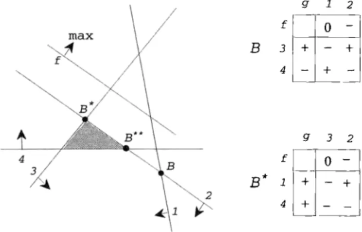
E x a m p l e 14. Consider the LP illustrated in Fig. I0. In this example, E = { 1 , 2 , 3 , 4 , f , g}, and the set of feasible solutions is the shaded triangle region. There are two optimal bases B* = { 1,4, f } and B** = { 1,3, f } . At the dictionary for the basis B = {3, 4, f } , there is only one admissible pivot, that is at (4, 1). Clearly by this pivot, one reaches the basis B**. Thus, the basis B* is not reachable from B by any admissible pivots.
The question becomes interesting once we assume nondegeneracy. We say that an LP basis B is
nondegenerate
ifdig 4 : 0
for all basic variable i E B - f . An LP basis B is said to bedual-nondegenerate
if the associated nonbasis is nondegenerate for the dual problem, or equivalentlydfj ~ 0
for all nonbasic variable j E N - g. Finally, an LP basisis fully nondegenerate
if it is both nondegenerate and dual-nondegenerate. One can easily prove the following.L e m m a 15.
I f L P has a fully nondegenerate optimal basis, then it is the unique optimal
basis.
Our main theorem in this section is the following which is a consequence o f the uniqueness lemma above.
Theorem 16.
If an
LPhas a fully nondegenerate optimal basis
B*,then there exists a
sequence of
I B* \ B[admissible pivots from any
LPbasis B.
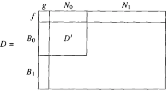
Proof. Let B* be a fully nondegenerate optimal basis for a given LP and let B be any L P basis different from B*. Set B0 = B \ B*, B1 = B* fq B, No = N \ N* = B* \ B and N1 = N* N N. Consider the submatrix D ' = O(Bo+f)(No+g) o f the dictionary D =
D ( B ) .
The matrix D ' represents a smaller linear optimization problem LP ' with variables B0 U No, see Fig. 11.
388 K. Fukuda, T. Terlaky/Mathematical Programming 79 (1997) 369-395 g No N1 f Bo D ~ D = Bl
Fig. 11. A partition of the dictionary D = D(B).
It is easy to see that LP ~ has a fully nondegenerate optimal basis, namely No + f , and by Lemma 15 it is a unique optimal basis. This implies that the basis B0 + f cannot be terminal. This together with Proposition 12(a) implies that there exists an admissible pivot in D ~. This transformation makes the resulting basis closer to the feasible basis B* by one. Hence, by applying the same argument, we can arrive at B* by a sequence of admissible transformations involving exactly [B* \ B I pivots. []
One might suspect that this theorem is a disguised form of a simple well-known lemma in linear algebra: any two bases B and B ~ of a matrix A can be connected by a sequence of IB' \ B{ pivot operations. As it was illustrated by Example 14, the validity of our theorem critically depends on the full nondegeneracy assumption, which has no counterpart in this lemma. Therefore we do not see any easy way to relate these two statements with similar appearances.
In order to apply the theorem to general degenerate LPs, we can use a standard technique of lexicographic (symbolic) perturbation to both the primal and the dual LP. This makes all LP bases fully nondegenerate symbolically, see [30] for details.
5. Conclusions and open problems
The goal of the present paper was to provide a good motivation to study a class of pivot algorithms which is more general than the class of simplex algorithms. This broader view on pivot methods resulted in a family of simple, finite, one-phase methods, it made possible to give simple constructive proofs for the LP strong duality theorem, and it allowed us to explore the combinatorial structures of linear optimization problems. New results on the existence of a short admissible pivot path were presented. This is a weaker analogue of the old, very difficult problem, the so-called d-step conjecture [47].
Some related open problems are sketched below.
The simplex method has been studied extensively by many researchers since it was invented in 1947 by Dantzig [ 21,23 ], but yet it resists the resolution of the long-standing open problem:
K. Fukuda, Z Terlaky/Mathematical Programming 79 (1997) 369-395 389 O p e n P r o b l e m 1. Is there any pivot rule for the simplex method which terminates in a number of pivots bounded by a polynomial in m and n?
Unfortunately this problem 1 seems to be too hard because the existence question: O p e n P r o b l e m 2. Is there a simplex-pivot path to an optimal basis from any given feasible basis whose length is bounded by a polynomial of m and n?
appears to be already too hard. Observe that a solution of the first problem gives a solution to the second one. Furthermore, the affirmative answer to this latter simpler question would imply the solution of the famous diameter problem of convex polytopes: O p e n P r o b l e m 3. Is the combinatorial diameter of a d-dimensional polytope with m- facets bounded by a polynomial in m and d?
Although some interesting results on the diameter of polytopes have been obtained recently (e.g. [41 ] ) , we must admit that we are still quite far from the solution to this "simpler" problem.
In Section 4 a positive answer to a much weaker question is presented. We have seen that if the optimal basis is fully nondegenerate, a short admissible pivot path from any basis to the optimal basis exists. This existence result raises the following more difficult question (posed by H.-J. Li.ithi):
O p e n P r o b l e m 4. For any given LP, is there an ordering of variables for which the least- index criss-cross method finds an optimal basis from any given basis in a polynomial number of pivots?
A much simplified question, which seems to be already hard, is:
Open
P r o b l e m 4 I. For any given LP, a given optimal basis and a given initial basis, isthere an ordering of variables for which the least index criss-cross method terminates in a polynomial number of pivots?
Although the least-index criss-cross method presented in Section 3 admits an expo- nential example, the ultimate goal of our study is of course to answer the most basic question:
O p e n P r o b l e m 5. Is there a polynomial criss-cross method?
Another open problem concerns the practicality of criss-cross rules. Contrary to the many efficient implementations of simplex methods, to date no practically efficient criss-cross method is known. Thus the following question remains.
390 K. Fukuda, T. Terlaky/Mathematical Programming 79 (1997) 369-395
Preliminary but interesting experimental results on some modifications of the least- index criss-cross method were presented in [58].
As we mentioned earlier, not much is known on the expected number of pivot steps of criss-cross methods. This is in sharp contrast to the extensive literature on the expected number o f steps of simplex methods.
Open P r o b l e m 7. What is the expected number of pivots required by a finite criss-cross method to solve an LP?
O f course this is not a single question. One can pose this question with respect to many different probabilistic models and with different criss-cross algorithms.
6. Historical n o t e s
6.1. Origins
From the early days of LP research, people have been looking for an algorithm that avoids the two phase procedure needed in the simplex method when solving the general LP problem. Such a method was assumed to rely on the intrinsic symmetry behind the primal and dual problems (self-dual), and it should be able to start with any basic solution.
There were several attempts made to relax the feasibility requirement in the sim- plex method. It is important to mention Dantzig's [22] parametric self-dual simplex algorithm. This algorithm can be interpreted as Lemke's [50] algorithm for the cor- responding linear complementarity problem [52]. In the sixties people realized that pivot sequences through possibly infeasible basic solutions might result in significantly shorter paths to the optimum. Moreover a self-dual one phase procedure was expected to make linear programming more easily accessible for broader public. Probably these advantages stimulated the birth of Zionts' [82,83] criss-cross method (after which the finite criss-cross methods discussed in this paper were named too).
R e m a r k 17
(Zionts' criss-cross method).
Assuming that the reader is familiar with both the primal and dual simplex methods, Zionts' criss-cross method can easily be explained.• It can be initialized by any, possibly both primal and dual infeasible basis. I f the basis is not optimal, then there are some primal or dual infeasible variables. One might choose any of these. It is advised to choose primal and dual infeasible variables alternately if possible.
• If the selected variable is dual infeasible, then it enters the basis and the leaving variable is chosen among the primal feasible variables in such a way that primal feasibility of these variables is preserved.
K. Fukuda, T. Terlaky/Mathematical Programming 79 (1997) 369-395 391 • I f the selected variable is primal infeasible, then it leaves the basis and the entering variable is chosen among the dual feasible variables in such a way that dual feasibility o f these variables is preserved.
If no such basis exchange is possible another infeasible variable is selected. If the current basis is infeasible, but none o f the infeasible variables allows a pivot fulfilling the above requirements then it is proved that the problem L P ( A , b , c ) has no optimal solution.
Once a primal or dual feasible solution is reached then Zionts' method reduces to the primal or dual simplex method respectively.
One attractive character o f Zionts' criss-cross method is primal-dual symmetry (self- duality), and this alone differentiates itself from the simplex method. However it is not clear 8 how one can design a finite version (i.e. a finite pivot rule) o f this method. Nevertheless, this is the first root o f the finite criss-cross methods studied in this paper. The other root o f finite criss-cross methods was the intellectual effort to find finite variants (other than the lexicographic rule [ 13,24] ) o f the simplex method and its specialized variants. These efforts were also stimulated by studying the combinatorial structures behind linear programming. From the early seventies in several branches o f the optimization theory, finitely convergent algorithms were published, and in partic- ular consistent labelling 9 and pivot selection rules based on least index ordering Io established a solid foundation for finite pivot algorithms.
The birth o f oriented matroids and oriented matroid programming [8,9,28] gave an essential impulse to this research. It became clear that although the simplex method has rich combinatorial structures, some essential results like the finiteness o f Bland's minimal index rule [8] cannot be proved in the oriented matroid context. In fact Edmonds and Fukuda [ 2 9 ] showed that it might cycle in the oriented matroid case due to the possibility o f nondegenerate cycling which is impossible in linear programming.
Interesting combinatorial pivot algorithms were discovered and mainly published in the oriented matroid context. A m o n g them are Bland's recursive algorithm [7,8], the E d m o n d s - F u k u d a algorithm [29] (the interested reader can find variants and general- izations in e.g. [6,16,75,76,80] ). All these methods in the linear case are variants o f the simplex method, i.e. they preserve the feasibility o f the basis. In contrast, in the case o f oriented matroid programming only Todd's finite lexicographic method [68,69] pre- serves feasibility o f the basis and therefore yields a finite simplex algorithm for oriented matroids. For a thorough survey on pivot algorithms the reader is referred to [67].
All these research results made the time ripe for the discovery o f finite criss-cross methods. It is remarkable that almost at the same time, in different parts o f the world
8 Because in some c~scs ZionLs" me~od reduces to the simplex method, lexicographic peaurbation or minimal index resolution is a must when one thinks about finiteness. However these do not ,seem to be sufficient to prove finiteness in the general case when the initial basis is both primal and dual infeasible.
9 See Tucker's [71 I consistent labelling technique in the Ford-Fulkerson flow algorithm
l°See Murty's 155 ] Bard-type scheme for the P-matrix linear complementarity problem and Bland's [81 celebrated least index rule in linear programming.
392 K. Fukuda, Z Terlaky/Mathematical Programming 79 (1997)369-395
(China, Hungary, USA) essentially the same result was obtained independently by approaching the problem from quite different directions.
6.2. Birth
The first finite criss-cross ',algorithm, which we called the least-index criss-cross method, was discovered independently by Chang [12], Terlaky [63,65,64] and Wang
[741 A strongly related general recursion was found by Jensen [40].
In his unpublished report [ 12] Chang presented in 1979 this algorithm for positive semidefinite linear complementarity problems as a generalization of Murty's [ 55 ] Bard- type scheme. He was studying the role of least index resolution of degeneracy problems in Lemke's algorithm [49,50] and in variants of the principal pivoting method [ 18] as one solves linear complementarity problems. If one specializes the algorithm on page 59 of his long report to the linear programming case, precisely the finite, least-index criss-cross method is obtained. Unfortunately this result remained unknown until the early nineties [38,72].
At the end of 1983, Terlaky presented the least-index criss-cross algorithm for LP [63,64] and then immediately generalized in 1984 to the oriented matroid case [65]. Since then the algorithm was known by the name "finite (or convergent) criss-cross method". This name was given due to the motivation from Zionts' [82] ideas. These papers inspired a good deal of research on criss-cross methods in the last decade.
Wang's motivation was quite different. He was working on oriented matroids and tried to resolve the problems arising from possible cycling of Bland's least index simplex algorithm in oriented matroids. In 1985 Wang [74] presented his version for oriented matroid programming under the name "a finite conformal elimination free algorithm" which again turned out to be the same finite criss-cross method.
Bland and his then Ph.D. student Jensen worked on the recursive line. Their research resulted in a general recursive scheme [40]. Jensen's "generalized relaxed recursive scheme" is actually a general model for finite pivot algorithms and it is easy to see that the least-index criss-cross method can be interpreted as a concrete realization of this general scheme.
Acknowledgements
The authors are grateful to Tibor Illds, Thomas M. Liebling, Hans-Jakob Ltithi, Kees Roos and Shuzhong Zhang for reading earlier versions of this paper and making useful comments that improved the presentation of the paper considerably.
References
[ 1 I I. Adler and N. Megiddo, A simplex algorithm whose average number of steps is bounded between two quadratic functions of the smaller dimension, Journal of the Association of Computing Machinery 32 (1985) 891-895.