HAL Id: hal-02281379
https://hal.archives-ouvertes.fr/hal-02281379
Submitted on 9 Sep 2019
HAL is a multi-disciplinary open access
archive for the deposit and dissemination of
sci-entific research documents, whether they are
pub-lished or not. The documents may come from
teaching and research institutions in France or
abroad, or from public or private research centers.
L’archive ouverte pluridisciplinaire HAL, est
destinée au dépôt et à la diffusion de documents
scientifiques de niveau recherche, publiés ou non,
émanant des établissements d’enseignement et de
recherche français ou étrangers, des laboratoires
publics ou privés.
Numerical study of the cryogenic cooling of amplifiers
for high power lasers
Morgane Bellec, Nicolas Luchier, Guillaume Balarac, Ulrich Bieder, Alain
Girard
To cite this version:
Morgane Bellec, Nicolas Luchier, Guillaume Balarac, Ulrich Bieder, Alain Girard. Numerical study of
the cryogenic cooling of amplifiers for high power lasers. The 14th International Conference on Heat
Transfer, Fluid Mechanics and Thermodynamics (HEFAT), Jul 2019, Wicklow, Ireland. �hal-02281379�
NUMERICAL STUDY OF THE CRYOGENIC COOLING OF AMPLIFIERS FOR HIGH POWER LASERS
Bellec M.1*, Luchier N.1, Balarac G.2, Bieder U.3 and Girard A.1
*Author for correspondence
1. Univ. Grenoble Alpes, CEA, IRIG, DSBT, Grenoble, France
2. Laboratoire des écoulements géophysiques et industriels (LEGI) - CNRS-UGA-G-INP, Grenoble, France 3. CEA, Université Paris-Saclay, DEN-STMF, Gif-sur-Yvette, France
E-mail: morgane.bellec@cea.fr
ABSTRACT
The French collaborative Trio4CLF project aims to understand and control the cryogenic cooling of amplifiers for high power (~1 PetaWatt) and high repetition rate (1-10 Hertz) lasers. In such amplifiers, the fluid (low temperature gaseous helium) evacuates the thermal power absorbed by the solid amplifying plates. A precise knowledge of the heat exchange and of the turbulent fluid flow in the amplifier is requested to evaluate its impact on the laser beam quality. Large Eddy Simulations representative of the amplifier cooling are performed using TrioCFD, a code developed by the CEA. First, validation simulations are carried out for heated periodic channel flows, allowing comparisons with Direct Numerical Simulation results from the literature. They are conducted using conjugate heat transfer calculation between the fluid and the solid. The channel flow is turbulent, with a bulk Reynolds number (based and the bulk velocity and the total height of the channel) of about 14000. Large Eddy Simulation of a heated open turbulent cryogenic helium flow with developing thermal boundary layers is then presented.
INTRODUCTION
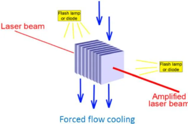
The thermal management of solid-state laser amplifiers has become a critical issue in order to increase the repetition rate of high power lasers [1]. A cryogenic cooling of the amplifier is especially interesting due to the better thermal and optical properties at low temperatures than at room temperature of the crystals used as amplification medium [2, 3]. To increase the heat transfer surface, the studied amplifier [4] has a slab configuration as shown in Fig. 1. It is cooled by a forced flow of gaseous helium.
In such configuration, the laser beam is perpendicular to the helium flow. Due to the low viscosity of cold helium, turbulence will develop in the flow. An inhomogeneous temperature field will produce inhomogeneity in the refractive index distribution through density variations. The effect on the laser beam coherence must be assessed. A similar problem occurs when a laser beam propagates through a compressible turbulent boundary layer, with the difference that the density variations are then induced by the pressure fluctuations rather than the temperature ones [5, 6]. Tromeur et al. [5] recommended the use of Large Eddy Simulations (LES) to correctly evaluate these aero-optical effects due to inaccuracies obtained when using
optical models combined with RANS simulations. Mani et al. [6] confirmed that a typical LES will correctly capture those effects.
Figure 1 Schematic view of the laser amplifier
Several numerical studies exist in the literature on fully developed turbulent channel flow with heat transfer. Kawamura
et al. [7] conducted Direct Numerical Simulations (DNS) at
different Prandtl and Reynolds numbers using a non-fluctuating temperature boundary condition at the walls, constituting a reference database. Bricteux et al. [8] conducted similar simulations in DNS and LES, in the specific case of a very low Prandtl number, typical for liquid metals. These studies overlooked the actual wall/fluid heat transfer by using ideal non-fluctuating temperature boundary condition. Tiselj et al. [9] conducted DNS of turbulent channel flow with conjugate heat transfer at different Reynolds numbers and for different solid and fluid properties. They showed that the thermal boundary condition has a small influence on the mean temperature and on the temperature heat fluxes, but that it affects the temperature fluctuations in the fluid. Conjugated heat-transfer is also used in more complex geometries such as channel flow with a wire embedded in one of the wall [10].
A step-by-step strategy is adopted. In the present study, LES are performed in conditions representative of a simplified cryogenically cooled laser amplifier, namely a turbulent channel flow of gaseous helium at 80 K between two crystal plates at 105 K. Validation simulations in a periodic channel are first presented to assess the quality of the simulations by comparison with DNS results of the literature. Since temperature fluctuations
are the quantity of interest, the crucial prediction of the heat transfer between the solid and the fluid is calculated by conjugated heat transfer. These calculations revealed that Dirichlet boundary conditions with imposed temperature lead to similar results. A LES of a heated open channel flow is then conducted using such imposed temperature boundary conditions. The developing thermal boundary layers are presented.
NOMENCLATURE
Cp [J/kgK] Heat capacity
G [m2/kg] Gladstone-Dale constant
h [m] Half-height of the channel
hexch [W/m2K] Heat transfer coefficient
k [rad/m] Wave number
L [m] Domain dimension m [kg] Mass n [-] Index of refraction N [-] Number of cells Nu [-] Nusselt number P [Pa] Pressure Pr [-] Prandtl number Q [W] Power q [K/s] Source term Re [-] Reynolds number S [m2] Exchange surface T [K] Temperature t [s] Time U [m/s] Velocity V [m3] Volume x [m] Streamwise axis y [m] Crosswise axis z [m] Spanwise axis Special characters α [m2/s] Thermal diffusivity λ [W/mK] Thermal conductivity λl [m] Wavelength ρ [kg/m3] Density 𝒯 [s] Time constant ν [m2/s] Kinematic viscosity
𝜙 [rad] Wave phase
Subscripts and superscripts
b Bulk
i Any Cartesian direction
f Fluid
RMS Root Mean Square
s Solid
τ Friction
w Wall
+ Normalization
NUMERICAL MODEL
All simulations were performed using TrioCFD [11], an open-source CFD code developed by the Nuclear Energy Division of CEA. Physical properties of the media, geometry of the calculation domain as well as thermohydraulic conditions of
the calculations are representative of a cryogenically cooled laser amplifier.
At a temperature of T=80 K and a pressure of P=5×10⁵ Pa,
helium is a gas with a kinematic viscosity ν=3×10⁻⁶ m2/s. The
half-height of the cooling channel, formed by the amplifier crystal plates, is h=2×10⁻³ m. The bulk velocity used for this
study is Ub=10 m/s, although typical velocities in laser amplifiers
could be 5 times higher. The flow is assumed to be turbulent and fully developed. The corresponding bulk Reynolds number 𝑅𝑒𝑏=
𝑈𝑏 2ℎ
𝜈 = 14000 corresponds to a friction Reynolds
number of 𝑅𝑒𝜏= 𝑢𝜏 ℎ
𝜈 = 400.
Treating turbulence by LES consists in resolving the large scale of turbulence while modelling the small scales. The scales are separated by filtering the conservation equations. A detailed description of this type of simulations can be found in [12]. The WALE subgrid scale model, developed by Nicoud & Ducros [13] is used as it is well adapted for wall-bounded flows. Wall functions are not used.
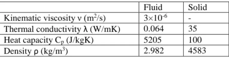
The energy of the laser is accumulated in the amplification crystals and evacuated by the helium flow. The heat balance of the flow shows that the mean temperature increase of the fluid between the inlet and the outlet of the domain is below 1.3 K. The impact of temperature variations on physical properties is neglected as it is of 1 to 2 %. The fluid properties are taken as constant and the temperature is considered as a passive scalar (Pr=0.70). The used fluid and solid properties are summarized in Table 1.
Table 1 Constant physical properties of fluid and solid
Fluid Solid Kinematic viscosity ν (m2/s) 3×10⁻⁶ - Thermal conductivity λ (W/mK) 0.064 35 Heat capacity Cp (J/kgK) 5205 100 Density ρ (kg/m3) 2.982 4583
For the fluid, the governing set of conservation equations in the filtered form, represented by ( )̃, are then for an incompressible flow: the conservation of mass (1), momentum (2) and energy (3). For the solid, the conservation of the energy is given in equation (4): ∂ũ𝑖 ∂x𝑖 = 0 (1) ∂ũ𝑖 ∂𝑡 + ∂ũ𝑖u𝑗 ∂x𝑗 =−1 𝜌𝑓 𝜕𝑃̃ 𝜕𝑥𝑖 + 𝜈 𝜕 𝜕𝑥𝑗 (𝜕𝑢̃𝑖 𝜕𝑥𝑗 +𝜕𝑢̃𝑗 𝜕𝑥𝑖 ) (2) ∂𝑇̃ ∂𝑡+ ∂ũ𝑖T ∂x𝑖 = α𝑓 𝜕2𝑇̃ 𝜕𝑥𝑖2 + 𝑞𝑓 (3) ∂T ∂𝑡= α𝑠 𝜕2𝑇 𝜕𝑥𝑖2 + 𝑞𝑠 (4)
The heat deposited by the pumping is taken into account via the term 𝑞 = 𝑄
𝐶𝑝×𝜌×𝑉 where Q is the heat source.
A 3rd order Runge-Kutta scheme is used for time integration.
The discretization in space is done by the MAC method of Harlow & Welsh [14], using 2nd order centered diffusion
schemes for momentum and energy. For dynamic convection, a 2nd order centered scheme is used. For thermal convection, a 3rd
order (QUICK) scheme is applied.
RESULTS OF THE NUMERICAL ANALYSIS
The results of the LES calculations are presented as non-dimensional quantities, normalized using the classical scaling method [12]: 𝑈+=〈𝑈〉 𝑈𝜏, 𝑈𝑖 𝑅𝑀𝑆 +=𝑈𝑖 𝑅𝑀𝑆 𝑈𝜏 , 𝑦 +=y 𝑈𝜏 𝜈 , 𝑇+=𝑇𝑤−〈𝑇〉 𝑇𝜏 , 𝑇𝑟𝑚𝑠 +=𝑇𝑟𝑚𝑠 𝑇𝜏 (5)
The velocities are normalized by the friction velocity, calculated from the wall normal gradient of the mean velocity:
𝑈𝜏 = √𝜈 (
𝜕〈𝑈〉 𝜕𝑦 )
𝑤
(6)
The temperatures are normalized by the friction temperature, calculated from the wall normal gradient of the mean temperature and the friction velocity:
𝑇𝜏=
𝜆 (𝜕〈𝑇〉𝜕𝑦 )
𝑤
𝜌𝐶𝑝𝑈𝜏
(7)
Heated periodic channel flow
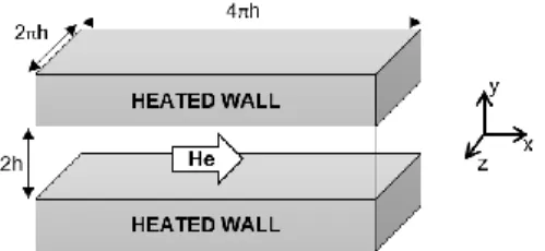
In the first step, the method to simulate conjugated heat transfer in a laser amplifier is validated by simulating by LES a streamwise (x) and spanwise (z) bi-periodic plane channel that is bounded crosswise (y) by two heated solid plates. The computational domain is shown in Fig. 2. The dimensions of the channel are Lx×Lfy×Lz = 4πh×2h×2πh. Both plates have the
streamwise and spanwise dimensions of the channel; their heights are Ls
y=3.5×10⁻³ m. The fluid mesh contains Nx×Nfy×Nz
= 120×192×240 cells. The cells are streamwise and crosswise homogeneously distributed with non-dimensional sizes of Δx+=40and Δz+=10, scaled by the friction velocity uτ. The mesh
is refined crosswise near the wall to Δy+=1. Starting at the wall,
the cells are gradually coarsen crosswise following a tangential hyperbolic law. The maximum cell size at the center of the channel is Δy+=15. The solid mesh contains Nsy=30
homogeneously distributed cells.
Figure 2 Computational domain with flow channel and heated
plates
Statistics are collected by averaging over the two homogeneity directions x and z, and over time. 0.1 s are
simulated for the statistics, which represents 30 characteristic times defined as h/Uτ.
Fig. 3 presents the crosswise profile of the normalized streamwise mean velocity U+ plotted with the normalized
distance to the wall y+. The comparison shows a satisfying
agreement with DNS results of Kawamura [7] realized at the same Reynolds number although the velocity is under-estimated in the center of the channel. This result can be improved by using a 4th order scheme for dynamic convection; the 2nd order scheme
was preferred for stability reasons.
Figure 3 Normalized mean streamwise velocity in the channel
flow, compared to DNS data of Kawamura et al. [7] Fig. 4 presents in the same way the normalized velocity fluctuations UiRMS+ in the three coordinate directions, which are
compared to the same DNS of Kawamura [7]. This comparison also shows a good agreement between DNS and LES.
Figure 4 Normalized root mean squares of velocity in the
channel flow, compared to DNS data of Kawamura et al. [7] In a first approach, a total thermal power of Qs=9.2 W is
deposited in the solid plates by a constant volume heat source. Qs is representative of a cryogenically cooled multi-slab
amplifier [15], proportionally to the simulated volume. In order to conserve the energy in the calculation domain, the same
thermal power is removed from the fluid by a constant volume source term (Qf= -Qs). The initial temperature of the solid has a
constant value of Ts=105 K and of the fluid of Tf=80 K.
In an actual laser, the thermal power is not deposited constantly in the amplifier but only during discrete nanosecond pulses with a typical frequency of 10 Hz [15]. The thermal balance in the solid is as follows:
𝑚𝑠𝐶𝑝𝑠
𝑑𝑇𝑠
𝑑𝑡 = 𝑄𝑠− 𝑆 × ℎ𝑒𝑥𝑐ℎ× (𝑇𝑠− 𝑇𝑓) (8) Where ms= (ρ× Lx×Ly×Lz)s is the solid mass, S=Lx×Lz is the
exchange surface and hexch is the heat transfer coefficient. This
leads to a thermal time constant: 𝒯 =(𝜌 × 𝐶𝑝× L𝑦)𝑠
ℎ𝑒𝑥𝑐ℎ
(9) The heat transfer coefficient can be approximated to hexch=600 W/m2K using the classical Dittus-Boelter correlation:
Nu=0.023Re0.8×Pr0.4 [16]. The thermal time constant is then
estimated to 𝒯=2.6 s. In other words, in 0.1 s (the time between two laser pulses) the solid temperature decreases by about 1 K, less than 4% of the fluid/solid temperature difference. These variations are here neglected by the constant heat source approximation and the simulation reaches a thermal equilibrium. 0.2 s were simulated to attain the thermal equilibrium prior to the 0.1 s simulated to collect the statistics.
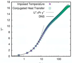
Fig. 5 and 6 respectively present the normalized mean temperature T+ and normalized the root mean square of
temperatures TRMS+ plotted with the normalized distance to the
wall y+. They are again compared to DNS results of Kawamura
[7]. The mean temperature profile shows an excellent agreement between LES and DNS while the temperature fluctuations are underestimated.
Figure 5 Normalized mean temperature in the heated periodic
channel flow with and without plates, compared to DNS data of Kawamura et al. [7]
The temperature fluctuations in the fluid tend to zero at the wall, while temperatures barely fluctuate in the solid plates: the temperature root mean squares range from 2×10⁻² K at the fluid
interface to 3×10⁻⁴ K at the opposite face. This is coherent with
the fluid and solid characteristics: the thermal activity ratio 𝐾 = √(λρCp)f⁄(λρCp)s=8. 10−3 is small, suggesting that the
fluid/solid interface behaving similarly to an ideal non-fluctuating temperature boundary condition [9].
To confirm the analogy, the same fluid channel was simulated using a Dirichlet boundary condition with imposed temperature of Tw=104.5 K at the wall. Tw corresponds to the
wall temperature of the solid plates in the conjugated heat transfer case. The results of the imposed temperature simulation are also plotted in Fig. 5 and 6. Both mean and fluctuating temperatures perfectly collapse with the results of the conjugated heat transfer simulation.
Figure 6 Normalized root mean square of temperature in the
heated periodic channel flow with and without plates, compared to DNS data of Kawamura et al. [7]
Heated open channel flow
In the actual amplifier, boundary layers will develop along the channel, which may affect the laser beam quality. Indeed, different parts of the laser beam will propagate through a different thickness of thermal boundary layer, and will therefore meet different refractive index variations, affecting their optical paths differently. If the optical paths difference is of the order of or higher to the wavelength, the laser beam loses its coherence.
The results obtained in a streamwise periodic channel flow do not give information on this thermal boundary layer development, and it is necessary to study a thermally open channel. The dynamic of the flow is however kept as a fully developed turbulent plane channel. To do so, a periodic isothermal channel is used as precursor to supply the entrance instantaneous velocity field, as shown in Fig. 7. The mesh characteristics are the same as in the previous case of a periodic channel simulation.
The previous validation simulations presented no difference in the temperature fluctuations between the conjugated heat transfer and the imposed temperature boundary condition simulations, for fluid and solid characteristics set to typical values of a laser amplifier. The open channel flow simulation
was therefore conducted using an imposed temperature boundary condition at the walls.
The wall temperature distribution was obtained by a RANS simulation of an open channel coupled with two amplifier plates. The wall temperature is spanwise homogeneous, and it varies streamwise as follows:
𝑇𝑤= 0.017 × (𝑥 ℎ⁄ ) 2
+ 0.46 × 𝑥 ℎ⁄ + 100 (10) The inlet fluid temperature is homogeneous at 80 K.
Figure 7 Computational domain with precursor channel and
heated open channel
Since the open channel is not streamwise homogeneous, the statistics are now collected by averaging spanwise and over time. Starting from the RANS solution, 0.05 s are simulated prior to 0.2 s (i.e. 60 characteristic times) for the statistics computation.
Fig. 8 and 9 respectively present the mean temperature T and the root mean square of temperatures TRMS on a (xy) surface, thus
highlighting the thermal boundary layers developments along the heated open channel. The helium flow enters the channel at T=80 K from the left and it is heated by the upper and lower walls as it flows to the right.
Figure 8 Mean temperature on a streamwise plane in the heated
open channel flow, with contour line at constant temperature T=81 K
The root mean square of temperature reach a maximum 3.5 K on streamwise strips close to the walls, where are also localized the maximum of velocity fluctuations. The temperature fluctuations widen toward the center of the channel as the thermal boundary layers thicken. It should be reminded from the validation simulations that the temperature fluctuations peaks may be underestimated.
Figure 9 Root mean square of temperature on a streamwise
plane in the heated open channel flow
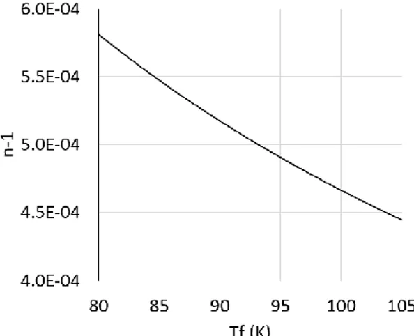
According to the Gladstone-Dale law, the index of refraction of a gas varies with its density following:
𝑛(𝑥, 𝑦, 𝑧) = 1 + 𝐺 × 𝜌(𝑥, 𝑦, 𝑧) (11) Where G is a constant. The helium temperature variations induce density variations and thus index of refraction variations shown Fig. 10. The index of refraction variations are small, confirming the choice of helium as coolant. Such small variations will not affect the laser beam amplitude, but they may induce a phase distortion.
Figure 10 Index of refraction variations in gaseous helium at
P=5.105 Pa and at low temperatures
The phase variation of a beam propagating crosswise through the channel flow is:
Δ𝜙(𝑥, 𝑧) = 𝑘 ∫ Δ𝑛(𝑥, 𝑦, 𝑧)𝑑𝑦
2ℎ 0
(12) Where Δ𝑛(𝑥, 𝑦, 𝑧) = 𝑛(𝑥, 𝑦, 𝑧) − 𝑛(0, 𝑦, 𝑧) is the variation of the refractive index compared to one at the inlet of the channel; and k=2π/λl is the wave number. For a Yb:YAG laser, the
wavelength is λl=940×10-9 m.
The mean temperature field is spanwise homogeneous in the simulated open heated channel. The phase variation induced by the mean temperatures varies monotonously between the inlet
and the outlet of the channel. The maximum phase variation is then Δ𝜙(12ℎ) = 0.3 rad.
It should be noted that this phase variation of 0.3 rad takes into account only one channel of the multi-slab configuration, and that only about a quarter of the actual channel length is here simulated. Moreover, only the mean temperature variations were considered, and the temperature fluctuations influence remains to be investigated.
CONCLUSION
Large Eddy Simulations were conducted in heated turbulent channel flows of low temperature gaseous helium. In a first step, the channel was streamwise periodic and it was crosswise bounded by two solid plates, using conjugated heat transfer. It was shown that for the physical characteristics representative of a cryogenically cooled laser amplifier, the mean and fluctuating temperatures results were similar to an ideal imposed temperature boundary condition simulation. To observe the thermal boundary layers developments, an open heated channel flow was then simulated using such wall thermal boundary condition. A first evaluation of the thermal boundary layer impact on the laser beam coherence was conducted for mean values. Large Eddy Simulation also gives access to the temperature fluctuations. They were computed along the heated channel, but their effect on the laser beam remains to be investigated. The next step will then consist in taking into account the dynamic boundary layers developments.
AKNOWLEDGEMENTS
This work was granted access to the HPC resources of CINES under the allocation 2019-A0052A10626 attributed by GENCI (Grand Équipement National de Calcul Intensif).
We acknowledge the financial support of the Cross-Disciplinary Program on Numerical Simulation of CEA, the French Alternative Energies and Atomic Energy Commission.
REFERENCES
[1] B. Le Garrec, “Laser-diode and Flash Lamp Pumped Solid-State Lasers,” in AIP Conference Proceedings, 2010, vol. 1228, pp. 111–116.
[2] V. Cardinali, E. Marmois, B. Le Garrec, and G. Bourdet, “Thermo-optical measurements of ytterbium doped sesquioxides ceramics,” in Proceedings of SPIE - The
International Society for Optical Engineering, 2010, vol.
7721, p. 77210U.
[3] D. Brown et al., “The Application of Cryogenic Laser Physics to the Development of High Average Power Ultra-Short Pulse Lasers,” Appl. Sci., vol. 6, no. 1, p. 23, Jan. 2016.
[4] J. P. Perin, F. Millet, B. Rus, and M. Divoký, “Cryogenic Cooling For High Power Laser Amplifiers,” presented at the 5th International Conference On The Frontiers Of Plasma Physics And Technology, Singapore, 2011.
[5] E. Tromeur, E. Garnier, and P. Sagaut, “Large-eddy simulation of aero-optical effects in a spatially developing turbulent boundary layer,” J. Turbul., vol. 7, p. N1, Jan. 2006.
[6] A. Mani, M. Wang, and P. Moin, “Resolution requirements for aero-optical simulations,” J. Comput. Phys., vol. 227, no. 21, pp. 9008–9020, Nov. 2008.
[7] H. Kawamura, H. Abe, and Y. Matsuo, “DNS of turbulent heat transfer in channel flow with respect to Reynolds and Prandtl number effects,” International Journal of Heat and
Fluid Flow, pp. 196–207, 1999.
[8] L. Bricteux, M. Duponcheel, G. Winckelmans, I. Tiselj, and Y. Bartosiewicz, “Direct and large eddy simulation of turbulent heat transfer at very low Prandtl number: Application to lead–bismuth flows,” Nucl. Eng. Des., vol. 246, pp. 91–97, May 2012.
[9] I. Tiselj and L. Cizelj, “DNS of turbulent channel flow with conjugate heat transfer at Prandtl number 0.01,” Nucl. Eng.
Des., vol. 253, pp. 153–160, Dec. 2012.
[10] E. Merzari, W. D. Pointer, J. G. Smith, A. Tentner, and P. Fischer, “Numerical simulation of the flow in wire-wrapped pin bundles: Effect of pin-wire contact modeling,” Nucl.
Eng. Des., vol. 253, pp. 374–386, Dec. 2012.
[11] P.-E. Angeli, U. Bieder, and G. Fauchet, “Overview of the TrioCFD code: main features, V&V procedures and typical applications to nuclear engineering,” in Proceedings of 16th
International Topical Meeting on Nuclear Reactor Thermal Hydraulics (NURETH-16), 2015.
[12] P. Sagaut, Large Eddy Simulation for Incompressible
Flows. Berlin, Heidelberg: Springer Berlin Heidelberg,
2002.
[13] F. Nicoud and F. Ducros, “Subgrid-scale stress modelling based on the square of the velocity gradient tensor,” Flow
Turbul. Combust., vol. 62, no. 3, pp. 183–200, 1999.
[14] F. H. Harlow and J. E. Welch, “Numerical Calculation of Time-Dependent Viscous Incompressible Flow of Fluid with Free Surface,” Phys. Fluids, vol. 8, no. 12, p. 2182, 1965.
[15] M. Divoky et al., “Conceptual design of 100 J cryogenically-cooled multi-slab laser for fusion research,”
EPJ Web Conf., vol. 59, p. 08004, 2013.
[16] F. W. Dittus and L. M. K. Boelter, “Heat transfer in automobile radiators of the tubular type,” Int. Commun.