HAL Id: hal-01344869
https://hal.archives-ouvertes.fr/hal-01344869
Preprint submitted on 12 Jul 2016
HAL is a multi-disciplinary open access
archive for the deposit and dissemination of sci-entific research documents, whether they are pub-lished or not. The documents may come from teaching and research institutions in France or
L’archive ouverte pluridisciplinaire HAL, est destinée au dépôt et à la diffusion de documents scientifiques de niveau recherche, publiés ou non, émanant des établissements d’enseignement et de recherche français ou étrangers, des laboratoires
Modelling the Variability of the Wind Energy Resource
on Monthly and Seasonal Timescales
Bastien Alonzo, Hans-Kristian Ringkjob, Benedicte Jourdier, Philippe
Drobinski, Riwal Plougonven, Peter Tankov
To cite this version:
Bastien Alonzo, Hans-Kristian Ringkjob, Benedicte Jourdier, Philippe Drobinski, Riwal Plougonven, et al.. Modelling the Variability of the Wind Energy Resource on Monthly and Seasonal Timescales. 2016. �hal-01344869�
Modelling the Variability of the Wind Energy Resource
on Monthly and Seasonal Timescales
Bastien Alonzo1,2,, Hans-Kristian Ringkjob1,2,4,, Benedicte Jourdier1,3,,
Philippe Drobinski1,, Riwal Plougonven1,, Peter Tankov2,
Abstract
An avenue for modelling part of the long-term variability of the wind energy resource from knowledge of the large-scale state of the atmosphere is inves-tigated. The timescales considered are monthly to seasonal, and the focus is on France and its vicinity. On such timescales, one may obtain information on likely surface winds from the large-scale state of the atmosphere, deter-mining for instance the most likely paths for storms impinging on Europe. In a first part, we reconstruct surface wind distributions on monthly and seasonal timescales from the knowledge of the large-scale state of the atmo-sphere, which is summarized using a principal components analysis. We then apply a multi-polynomial regression to model surface wind speed distribu-tions in the parametric context of the Weibull distribution. Several methods are tested for the reconstruction of the parameters of the Weibull distribu-tion, and some of them show good performance. This proves that there is a significant potential for information in the relation between the synoptic circulation and the surface wind speed. In the second part of the paper, the knowledge obtained on the relationship between the large-scale situation of the atmosphere and surface wind speeds is used in an attempt to fore-cast wind speeds distributions on a monthly horizon. The forefore-cast results are promising but they also indicate that the Numerical Weather Prediction seasonal forecasts on which they are based, are not yet mature enough to
Email address: bastien.alonzo@lmd.polytechnique.fr (Bastien Alonzo)
1IPSL/LMD, CNRS, Ecole Polytechnique, Universit´e de Paris-Saclay, Palaiseau, France 2Laboratoire de Probabilit´es et Mod`eles Al´eatoires, Universit´e Paris Diderot - Paris 7, Paris, France.
3EDF, R&D, Chatou, France
provide reliable information for timescales exceeding one month.
Keywords: Seasonal modelling, Wind distribution, Variability, large-scale circulation, Forecasts, Wind energy
1. Introduction
1
Owing to a well-established technology and the ever stronger push
to-2
wards replacing fossil fuels with clean renewable power, wind energy has
3
seen a dramatic growth in the recent years. According to the European
4
Wind Energy Association, about 12.8 GW of wind power was installed in
5
the European Union (EU) in 2015, bringing EUs total installed capacity to
6
141.6 GW. This corresponds to an electricity generation sufficient to cover
7
11.4 % of the EUs electricity consumption during an average year [1].
8
With the growing importance of wind energy, the interest and demand
9
for forecasts of the wind speed near the surface has seen a major boost.
10
Numerous methods exist for forecasting the wind speeds at different forecast
11
horizons implying different applications [2, 3]. Many studies focus on the
12
short-term scale ranging from several minutes to 1 day [4, 5, 6].
Medium-13
term forecast methods, ranging from several days up to 10 days, have also
14
been well investigated [7, 8, 9]. On much longer timescales and with very
15
different implications and motivations, the impact of climate change on wind
16
speeds has also been addressed [10, 11, 12].
17
By contrast, the intermediate timescale ranging from one month to a
18
season (hereafter referred to as long-term) has received only little attention.
19
Monthly and seasonal forecasts can be very useful for example in
mainte-20
nance planning, financial estimates and predictions of electricity generation
21
for network management. Some studies showed good results in forecasting
22
the monthly mean wind speed at several observation sites by using Artificial
23
Neural Network models (ANN) [13, 14], giving an acurate trend of the wind
24
speed at the yearly horizon, but a limited information on the wind variability
25
at higher frequency. Other authors forecasted daily mean wind speed at the
26
seasonal scale using ANN [15, 16, 17] allowing to gather more informations on
27
the wind variability inside a given season and which would allow to evaluate
28
the energy production. The ANN output is a predicted wind time serie. They
29
calculate the error regarding the real wind speed and compare the results to
30
other ANN [15, 16] or other statistical methods namely ARIMA models [17].
31
As ANN behaves like black box which we feed with data, the results are
difficult to explain physically. Moreover, each methods focuses on different
33
observation sites giving a limited idea of the spatial variations of the method
34
performance. Even though there are very few works on seasonal forecasts
35
of wind speeds, seasonal forecasting of other meteorological quantities is a
36
popular research topic with continuous improvement. For example, there
37
have been many works on seasonal forecasts of recurrent oscillating patterns
38
in the atmosphere, such as the El Nino [18, 19].
39
This paper focuses on modelling the wind variability on the long-term
40
timescale and makes an attempt of long-term wind speed distribution
fore-41
casting. The method proposed in this work aims to use the information found
42
in the large-scale configuration of the atmosphere in order to reconstruct
ex-43
pected distribution of surface winds. This paper answers some questions that
44
arise from this topic :
45
• How much information on the monthly or seasonal distribution of
sur-46
face winds can we obtain from knowledge of only the large-scale state
47
of the atmosphere?
48
• Are the proposed methods performing better than the climatology in
49
reproducing the surface wind speed distribution, and in estimating the
50
electricity generation?
51
• Do seasonal forecasts from an operational center of weather production
52
contain relevant information for an attempt of forecasting wind speed
53
distributions and electricity generation?
54
To address these questions in a consistent framework, we use data from
55
the European Center for Medium-Range Weather Forecasts (ECMWF).
In-56
deed, surface winds from ECMWF reanalysis have been shown to well
re-57
produce the observed surface winds in France [20]. Using reanalysis data
58
allows a better investigation of the statistical relation between local surface
59
winds and the large-scale circulation variability, especially because they
pro-60
vide a continuous description of surface wind speed over a wide domain and
61
over long time period. We focus on France and its vicinity not only because
62
the reanalyzed winds had been assessed there, but also because France has
63
a significant wind energy potential and interestingly includes regions with
64
different wind regimes. In Northern France the wind energy potential stems
65
from the storm tracks, whereas local orographic effects and channeling play
66
a major role in strong wind events of Southern France [21].
In the first part of this paper, the data and methodology used to link
68
the large scale circulation with the surface wind speed and to reconstruct
69
its monthly/seasonal distributions is described. Then, the performance of
70
the proposed methods is evaluated by comparing their results to the
clima-71
tology distributions. The performance is evaluated in terms of recontructed
72
electricity generation as well. In the last part of the paper, an attempt in
73
forecasting wind speed distributions and electricity generation is discussed.
74
2. Data and Methods
75
2.1. Data
76
ERAI reanalysis. Wind speed, geopotential height at 500hPa (Z500) and
77
Mean Sea Level Pressure (MSLP) are collected from ERA-Interim
reanal-78
ysis (ERAI, [22]) with a time-step of six hours during 35 years between
79
01/01/1979 and 12/31/2013, and then averaged to daily data. The
horizon-80
tal resolution of ERAI is 0.75◦ in latitude and longitude. Z500 and MSLP
81
span the North Atlantic and European grid (20◦N to 80◦N and 90◦W to
82
40◦E), and the surface wind speeds are obtained for a domain encompassing
83
France (40.5◦N to 52.5◦N and −6.75◦W to 10.5◦E).
84
The ERAI reanalysis data act as the reference data for wind speed. B.
85
Jourdier [20] showed that the ERA-Interim reanalysis has a good skill for
86
wind speeds in France, and is the best in comparison to two other reanalyses:
87
MERRA and the NCEP/NCAR. To reconstruct the distribution of the wind,
88
a 20 years calibration period, on which we train our methods, has been
89
defined from 1 January 1979 to 31 December 1998. Then a validation period
90
lasting 15 years from 01 January 1999 to 31 December 2013 follows.
91
ECMWF Forecasts. In the forecast section, the full 35 years period of ERAI
92
is used as a calibration period, while the period of forecast is always of 3
93
months, permitting to predict either monthly or seasonal distribution of the
94
surface wind speed. We retrieve twelve seasonal forecast sets of ECMWFs
95
numerical weather prediction model [23], from the years 2012, 2013 and 2014,
96
each lasting three months, starting from January, April, July and October.
97
Each set is composed of 41 seasonal forecast members from which we compute
98
the most likely scenario. This scenario is used as the only forecasted state
99
of the atmosphere. We apply the same methods using the 35 years of ERAI
100
to learn the relation between the surface wind speed and the large-scale
101
circulation of the atmosphere, and apply this relation to the forecasted state
102
of the atmosphere to predict wind speed distribution.
2.2. Methods
104
At a monthly to seasonal timescale, the surface wind speed is mainly
ex-105
plained by the large scale circulation of the atmosphere. The geopotential
106
height at 500hPa (Z500) and the Mean Sea Level Pressure (MSLP) are
vari-107
ables that well summarize this circulation. In this paper, we only present the
108
results of reconstruction using the Z500 variable as a predictor of the surface
109
wind speed. Indeed, results found when adding MSLP to Z500 predictor were
110
comparable and the improvement was neither systematic nor significant.
111
In the following paragraphs, we describe in detail the reconstruction
112
methodology which is summarized in Figure 1.
113
Our attempt aims at reconstructing the distribution of winds on the
114
monthly to seasonal timescales, but not at reconstructing daily timeseries
115
of winds. Indeed, our reconstruction methodology is based on the
prin-116
cipal components analysis of the Z500 predictor which informs about the
117
large-scale state of the atmoshpere. This knowledge will constrain the likely
118
distribution of surface winds on timescales larger than the lifetime of
indi-119
vidual synoptic systems (fronts, storms) and thus will not allow to
recon-120
struct such high frequency timeseries. Following the common practice, we
121
use the Weibull distribution to summarize the surface wind speed distribution
122
[24, 25].
123
Principal component analysis. To obtain a more compact representation of
124
the large-scale situation we perform a Principal Component Analysis (PCA)
125
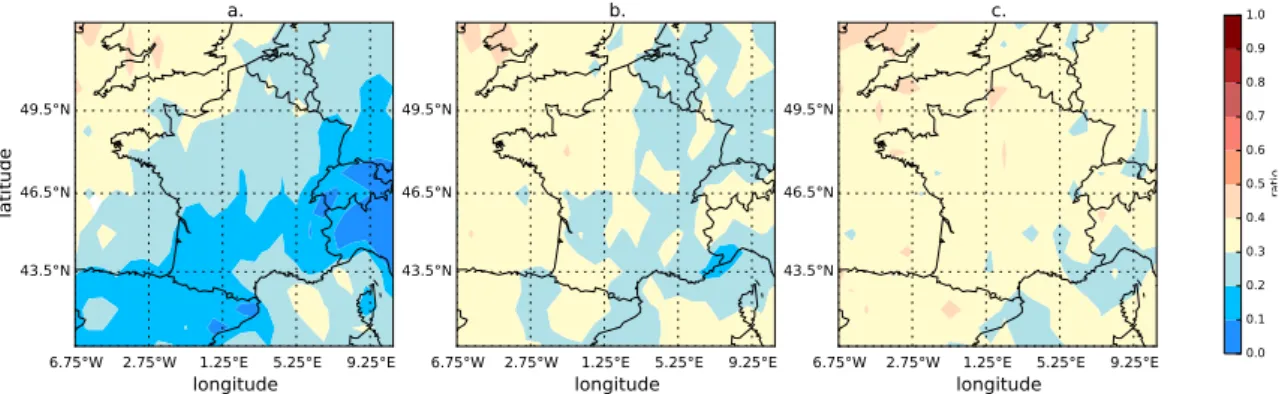
on Z500. It results in a set of Empirical Orthogonal Functions (EOF), which
126
represent the typical oscillation patterns spanning the North Atlantic
do-127
main. Each EOF is associated with one scalar timeseries (the corresponding
128
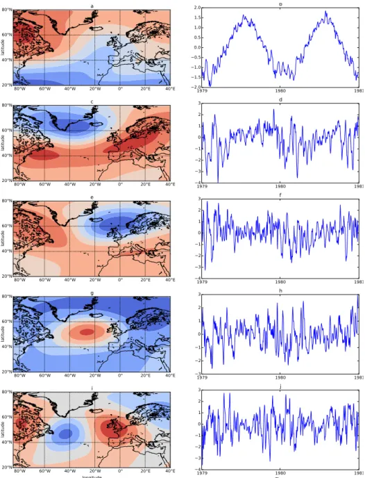
PC) which describes how each pattern evolves in time. Figure 2 shows the
129
five first EOFs and their associated PCs.
130
The first PC corresponds to the seasonal cycle (Fig 2. a,b), explaining
131
as much as 54.1% of the variance in the dataset: in winter the meridional
132
pressure gradient strengthens, leading to stronger winds and more intense
133
synoptic systems. The following four PCs have a clear physical interpretation
134
[26, 27], they all be related to teleconnection patterns, respectively the North
135
Atlantic Oscillation (NAO) (Fig 2. c,d), the Eastern Atlantic Pattern (EA)
136
(Fig 2. e,f), the Scandinavian pattern (SCA) (Fig 2. g,h) and the 2nd
137
European pattern (EU2) (Fig 2. i,j). These five first PCs explain 76.9% of
138
the variance in the entire dataset.
139
Weibull distribution. To summarize the wind distributions, we choose the
140
Weibull distribution as the parametric representation for montly and seasonal
141
distribution of the surface wind speed at a given location. This theoretical
142
distribution is widely used in the wind energy industry [28, 29, 24]. It
pro-143
vides a simple way to represent the wind distribution as it is based on only
144
two parameters: the shape parameter and the scale parameter. We must
145
highlight the fact that other theorical distributions better capture the shape
146
of the real wind distribution. In particular, the Rayleigh-Rice distribution
147
can have two modes, which is not the case for the Weibull [21].
148
The probability density function (PDF) and the cumulative distribution function (CDF) of the Weibull distribution are expressed as follows.
f (u; k, c) = k u (u c )k e−(u/c)k (1) F (u; k, c) = 1− e−(u/c)k, (2) where u is the wind speed, k and c are respectively the shape and the scale
149
parameter.
150
We now define three ways to reconstruct the parameters k and c from the data. The WAsP method, referred in the following as WAsP [30], computes
these parameters from the moments U and U3, as well as the probability of
lat itu de 80°W 60°W 40°W 20°W 0° 20°E 40°E 20°N 40°N 60°N 80°N a 1979 1980 1981 −2.0 −1.5 −1.0 −0.5 0.0 0.5 1.0 1.5 2.0 b lat itu de 80°W 60°W 40°W 20°W 0° 20°E 40°E 20°N 40°N 60°N 80°N c 1979 1980 1981 −4 −3 −2 −1 0 1 2 3 d lat itu de 80°W 60°W 40°W 20°W 0° 20°E 40°E 20°N 40°N 60°N 80°N e 1979 1980 1981 −4 −3 −2 −1 0 1 2 3 f lat itu de 80°W 60°W 40°W 20°W 0° 20°E 40°E 20°N 40°N 60°N 80°N g 1979 1980 1981 −3 −2 −1 0 1 2 3 h longitude lat itu de 80°W 60°W 40°W 20°W 0° 20°E 40°E 20°N 40°N 60°N 80°N i 1979 1980 1981 Time −4 −3 −2 −1 0 1 2 3 j
Figure 2: Five firsts EOFs (left side) and five first PCs (right side) of the PCA performed on the 35years and on the entire domain of ERAI Z500 dataset
data). The method focuses on the right-hand tail of the Weibull distribution, which is an important part of the distribution in terms of energy [31]. This
is why the WAsP method is preferred amongst the wind energy industry. In this method, k and c are calculated by solving the following equations.
U3 U3Γ ( 1 + 3 k )k 3 =−ln(1 − P (U)) (3) c = 3 √ U3 Γ(1 + k3) (4)
In a second method, referred in the following as KCrec, we take advantage of the fact that the Weibull distribution is given by two parameters, k and
c, and straightforwardly reconstruct these: they are fitted by the Maximum
Likelyhood Estimator (MLE) [32] on the calibration period. The MLE of the Weibull parameters is defined by the following equations.
∑n i=1u k i ln(ui) ∑n i=1uki − 1 k − 1 n n ∑ i=1 ln(ui) = 0, (5) c = ∑n i=1uki n . (6)
A last method was introduced in order to take into account how spread out the wind distribution is. This method, referred in the following as Perc,
uses two values, F (u1) and F (u2), of the Weibull distribution function,
cor-responding to wind speeds u1 and u2. The Weibull k and c parameters are
then given explicitly by:
c = ln ln( 1 1−F (u2)) ln(u1)− ln ln( 1 1−F (u1)) ln(u2) ln ln(1−F (u1 2))− ln ln( 1 1−F (u1)) , (7) k = c u1 ln ln( 1 1− F (u1) ). (8)
In order to determine the optimal values of u1 and u2, a synthetic test was
151
performed. First, we generated 30 (one month) or 90 (one season) samples
152
from the reference Weibull distribution with parameters k = 2 and c = 3.5.
153
Next, we determined the two Weibull parameters from the simulated samples
154
using the Perc method, using different combinations (u1, u2). To find the
155
best combination, we compared the resulting distributions with the reference
156
distribution using the Cramer-von Mises (CvM) score (see Appendix). It
157
was found that the best combination on a monthly scale is the 11th and 83rd
percentile. On the seasonal scale, the optimal combination is the 17th and
159
the 92nd percentile. The combination of the percentiles was not found to be
160
very sensitive, as there was a small region around the optimum combination
161
with very similar scores.
162
Multi-polynomial regression. We propose to link the large-scale situation
163
and surface wind speed distribution by a multi-polynomial regression
tak-164
ing the monthly mean PCs as explanatory variables and the parameters of
165
the Weibull distribution as dependent variables:
166 ˜ P = β0+ N ∑ n=1 βn,nCn(t)2+ N∑−1 n N ∑ m=n+1 βn,mCn(t)Cm(t). (9)
Here, ˜P is the dependent variable (Weibull parameter k or c for a given
loca-167
tion), Cn are the principal components and βn,n and βn,m are the regression
168
weights found by least squares. The number N of principal components is
169
determined by cross validation as explained below. We perform the
regres-170
sion on a calibration period of 20 years between 1979 and 1998. This results
171
in weights quantifying the relationship between the large-scale circulation
172
and the Weibull parameters for each individual location. These weights can
173
be combined with the known PC values on the reconstruction period of 15
174
years between 1999 and 2013 to reconstruct the monthly/seasonal Weibull
175
distribution.
176
Optimizing the number of principal components through cross validation. The
177
first five PCs of the Z500 can be easily interpreted as predictors of the wind.
178
Still, to a certain extent, the following PCs can also explain the variability of
179
the wind at the monthly/seasonal scale. To check whether taking five PCs is
180
really optimal, we performed a cross-validation procedure. For this purpose,
181
we calculated the temporally and spatially averaged CvM score (see
Ap-182
pendix) of 7 reconstructions of 5 years each, taking the remaining 30 years of
183
the data set as calibration period. Figure 3 plots the CvM scores as function
184
of the number of PCs used. The minimum mean CvM is clearly apparent
185
for all three methods for both monthly (Fig 3. a, b, c) and seasonal (Fig 3.
186
d, e, f,) reconstruction. This minimum is around five PCs which confirms
187
the fact that the large-scale circulation variability is accurately linked to the
188
wind speed variability at the monthly and seasonal timescale.
2 3 4 5 6 7 8 9 0.36 0.37 0.38 0.39 0.40 0.41 Me an Cv M sc ore a 2 4 6 8 10 12 14 0.27 0.29 0.31 0.33 b 2 4 6 8 10 12 14 0.25 0.27 0.29 0.31 0.33 c 2 3 4 5 6 7 8 9 Number of PCs 0.6 0.7 0.8 0.9 1.0 1.1 Me an Cv M sc ore d 2 4 6 8 10 12 14 Number of PCs 0.2 0.3 0.4 0.5 0.6 0.7 0.8 0.91.0 e 2 4 6 8 10 12 14 Number of PCs 0.2 0.3 0.4 0.5 0.6 0.7 0.8 0.9 1.0 f
Figure 3: Mean CvM score obtained by cross validation in function of the number of PCs used to reconstruct the distribution of the surface wind speed. From left to right: Wasp (a,d), Perc (b,e), and KCrec (c,f) methods; top: CvM score for monthly wind distribution reconstruction (a,b,c); bottom: CvM score for seasonal wind distribution reconstruction (d,e,f)
3. Evaluating the reconstruction methods
190
As mentionned in the Introduction, we use the wind speed from the
ERAI-191
reanalysis as the reference wind speed. To assess the reconstruction quality,
192
the CvM score (see Appendix) is calculated between the reconstructed CDF
193
and the real wind CDF. The CvM scores of the reconstructed wind speed
194
distributions are then compared to the CvM scores computed between the
195
real wind distributions and the climatological distributions. In simple terms,
196
the climatological distribution is the distribution of all values of wind for each
197
month or season in one specific location, based on all reanalysis data from this
198
location and the specific month or season. The climatological distributions
199
are usually used by the industry to have a first assessment of the wind energy
200
production at a seasonal time scale. An example of real, climatological and
201
reconstructed wind speed CDFs is shown in Figure 4.
202
3.1. Performance of methods for wind speed distribution reconstruction
203
The CvM score allows to test the null hypothesis (H0) that the two
sam-204
ples come from the same distribution. Assuming that the reconstructed
0 2 4 6 8 10 12 14 16 18 Surface wind speed (m/s)
0.0 0.2 0.4 0.6 0.8 1.0 Cu mu lat ive de nsi ty
Clim
Wasp
Perc
KCrec
Real
Figure 4: Real, climatological, and reconstructed seasonal CDFs for winter 2012 at 48.5◦N 3.0◦W
distributions and the real distributions are based on samples large enough to
206
say that the corresponding CvM scores follow the limiting distribution, we
207
can define the p-value corresponding to 95% confidence (see Appendix). If
208
the calculated CvM score is below this value, we can say at 95% confidence
209
that the two compared samples come from the same distribution. We
com-210
pare results of the tests for the climatology and the reconstruction methods.
211
We can define five different cases:
212
• Case A: H0 is not rejected for the method and rejected for the
clima-213
tology
214
• Case B: H0 is not rejected for both and the CvM of the method is
215
smaller than the CvM of the climatology
216
• Case C: H0 is not rejected for both and the CvM of the method is
217
larger than the CvM of the climatology
218
• Case D: H0 is rejected for the method and not rejected for the
clima-219
tology
220
• Case E: H0 is rejected for both the method and the climatology
Results over the whole domain in all different cases are given in table 1
222
and 2 for monthly and seasonal reconstruction respectively. We compare the
223
reconstruction methods to not only the classical climatology (a), but also to
224
the parametric climatology (b).
225
Indeed, the hypothesis of the Weibull distribution introduces a bias in the
226
distribution reconstruction which is not present in the classical climatology.
227
In order to have a fair comparison, we also fit by MLE a Weibull distribution
228
on the historical data referred as the parametric climatology.
229
Methods Wasp Perc KCrec Clim Parametric Clim
CvM < p 69.1 82.1 85.2 89.3 81.7 Comparison with a b a b a b - -Case A 5.8 11.5 6.5 11.9 6.9 13.0 - -Case B 17.8 24.1 25.0 34.0 27.3 37.1 - -Case C 45.5 33.5 50.5 36.2 51.1 35.1 - -Case D 26.0 24.1 13.8 11.6 11.2 9.5 - -Case E 4.8 6.8 4.1 6.3 3.7 5.3 -
-Table 1: Percentage of time the result of the CvM test gives Cases A,B,C,D, or E on the whole domain, for the entire validation period, for monthly reconstructed distribution compared to the classical climatology (a) and to the parametric climatology (b). The p-value, p, is 0.46136 for 95% confidence level (see appendix)
Methods Wasp Perc KCrec Clim Parametric Clim
CvM < p 44.3 73.3 79.8 88.6 77.3 Comparison with a b a b a b - -Case A 3.8 8.9 5.5 11.0 6.1 13.9 - -Case B 10.5 13.6 22.8 31.2 23.8 34.2 - -Case C 30.0 21.9 45.0 31.1 49.9 31.7 - -Case D 48.1 41.9 20.8 15.0 14.9 11.4 - -Case E 7.5 13.8 5.9 11.7 5.3 8.8 -
-Table 2: Same as table 1 but for seasonal distribution
The first lines of tables 1 and 2 show the fraction of time each method
230
gives a distribution not discernable from the real distribution at 95%
con-231
fidence level. It shows that all methods, appart from Wasp, have a good
232
ability to reconstruct the real wind distribution. We can also see that
fit-233
ting a Weibull distribution on the climatology reduces by about 10% this
234
percentage. Cases A and B summarize the number of time each method is
doing better than the climatology (non-parametric (a) or parametric (b)).
236
On the contrary, Cases C and D summarize the number of time the
cli-237
matology is doing better than the method. On average, on the all domain
238
and for monthly and seasonal timescales, the non-parametric climatology (a)
239
do better than every methods more than 60% of the time (78.1% against
240
Wasp at the seasonal scale, to 62.3% against KCrec at the monthly scale).
241
Nevertheless, when comparing to the parametric climatology, for monthly
242
and seasonal reconstruction, the KCrec method performs 49.1% of the time
243
better at monthly scale, and 48.1% at the seasonal scale. This shows again
244
the error brought by the Weibull distribution reconstruction. In all cases,
245
methods perform better at the monthly scale than at the seasonal scale. It
246
is interesting to notice that the cases for which the percentage is increased
247
at the seasonal scale are cases D and E, corresponding to times when
recon-248
structed distribution cannot be believed to come from the same distribution
249
as the real sample, at 95% confidence level. (Tables 1 and 2).
250
Figure 5 and 6 show on average on the validation the number of time
251
each method behaves better than the classical climatology (Cases A and B).
252
It can be seen that the Perc and KCrec methods do better than the Wasp
253
method. Indeed, at monthly timescale, the Perc and KCrec methods can
254
do better than the climatology in average more than 30% of times, while
255
the Wasp method does better than the climatology about 25% of times on
256
average displaying a clear difference between north and south (Figure 5 and
257
Table 1). On a seasonal scale, the Wasp method performs clearly worse
258
than at a monthly scale. The Perc and KCrec methods at a seasonal scale
259
display an interesting spatial variability. Indeed, they do more than 40%
260
of times better than the climatology in the north of France, whereas in the
261
south, this percentage is about 20% to 25% (Figure 6). When comparing
262
to the parametric climatology, all methods display the same pattern, but all
263
percentages are increased more than 10% (Not shown).
264
We can argue that the climatology does not reproduce well the extremes
265
of the wind distribution that is to say the strongest winds because it acts as
266
a filter of high frequency wind variations. In the northern part of France,
267
the storm track in winter and autumn brings stronger winds than in spring
268
and summer. We can assume that the reconstruction methods based on the
269
PCs of Z500 may better reproduce those strong winds than the climatology,
270
because the storm track position and strength is mainly driven by the NAO
271
and SCA oscillation patterns. Figure 7 shows the ratio of the number of times
272
each method is doing better than the climatology for seasonal distributions,
longitude
la
ti
tu
de
6.75°W 2.75°W 1.25°E 5.25°E 9.25°E
43.5°N 46.5°N 49.5°N
a.
longitude
6.75°W 2.75°W 1.25°E 5.25°E 9.25°E
43.5°N 46.5°N 49.5°N
b.
longitude
6.75°W 2.75°W 1.25°E 5.25°E 9.25°E
43.5°N 46.5°N 49.5°N c. 0.0 0.1 0.2 0.3 0.4 0.5 0.6 0.7 0.8 0.9 1.0 ra ti o
Figure 5: Fraction of times each method does better than the climatology (cases A and B) for monthly distribution reconstruction. From left to right: Wasp (a), Perc (b), KCrec (c) longitude la ti tu de
6.75°W 2.75°W 1.25°E 5.25°E 9.25°E
43.5°N 46.5°N 49.5°N
a.
longitude
6.75°W 2.75°W 1.25°E 5.25°E 9.25°E
43.5°N 46.5°N 49.5°N
b.
longitude
6.75°W 2.75°W 1.25°E 5.25°E 9.25°E
43.5°N 46.5°N 49.5°N c. 0.0 0.1 0.2 0.3 0.4 0.5 0.6 0.7 0.8 0.9 1.0 ra ti o
Figure 6: Same as Figure 5 but for seasonal distribution reconstruction.
by taking each season separately. We can clearly see on this figure that
274
the performance regarding the climatology of the Perc and KCrec methods,
275
and to a certain extent the Wasp method, depends on the season and on
276
the region. Indeed, both the Perc and the KCrec methods display a high
277
percentage of times (up to 70% at some points) when they do better than
278
the climatology in the north of France for the winter and autumn seasons.
279
3.2. Performance of the methods for estimating the capacity factor
280
For wind energy purposes, it is not exactly the full wind distribution that
281
needs to be estimated. For a given turbine, once the wind is between the
282
nominal wind speed and below the cut-out speed, the precise value does not
283
matter. In the present section we take this into account and reevaluate each
la
ti
tu
de
6.75°W 2.75°W 1.25°E 5.25°E 9.25°E
43.5°N 46.5°N 49.5°N
a.
6.75°W 2.75°W 1.25°E 5.25°E 9.25°E
43.5°N 46.5°N 49.5°N
b.
6.75°W 2.75°W 1.25°E 5.25°E 9.25°E
43.5°N 46.5°N 49.5°N
c.
6.75°W 2.75°W 1.25°E 5.25°E 9.25°E
43.5°N 46.5°N 49.5°N d. la ti tu de
6.75°W 2.75°W 1.25°E 5.25°E 9.25°E
43.5°N 46.5°N 49.5°N
e.
6.75°W 2.75°W 1.25°E 5.25°E 9.25°E
43.5°N 46.5°N 49.5°N
f.
6.75°W 2.75°W 1.25°E 5.25°E 9.25°E
43.5°N 46.5°N 49.5°N
g.
6.75°W 2.75°W 1.25°E 5.25°E 9.25°E
43.5°N 46.5°N 49.5°N h. longitude la ti tu de
6.75°W 2.75°W 1.25°E 5.25°E 9.25°E
43.5°N 46.5°N 49.5°N
i.
longitude
6.75°W 2.75°W 1.25°E 5.25°E 9.25°E
43.5°N 46.5°N 49.5°N
j.
longitude
6.75°W 2.75°W 1.25°E 5.25°E 9.25°E
43.5°N 46.5°N 49.5°N
k.
longitude
6.75°W 2.75°W 1.25°E 5.25°E 9.25°E
43.5°N 46.5°N 49.5°N l. 0.0 0.1 0.2 0.3 0.4 0.5 0.6 0.7 0.8 0.9 1.0 ra ti o
Figure 7: Fraction of time each method do better than the climatology (cases A and B) for seasonal distribution reconstruction based on Z500 for each season. From left to right: Winter, Spring, Summer and Autumn; From top to bottom: Wasp, Perc,and KCrec methods
method. A preliminary step consists in designing a procedure which mimicks
285
the weighting of wind values by a power curve, in a manner which accounts
286
for the considerable geographical variations of the wind (a single, generic
287
power curve would not make sense).
288
Each wind turbine is characterized by its power curve which gives the
289
output power as function of the wind speed. The energy produced during a
290
given period can be expressed as :
291
E = T
∫ ∞
0
Pout(u)dU, (10)
where T is the period considered (month or season) and Pout(u) is the output
292
power given the wind speed u. The capacity factor is defined as the ratio
between the actual energy produced during a given period and the energy
294
that would have been produced if the wind turbine had run at its maximum
295
power during the entire period :
296
CF = E PnT
, (11)
where Pn is the nominal power of the wind turbine.
297
In order to take into account the fact that the data used are at 10-meter
298
height and the mean wind speed is highly varying among different locations,
299
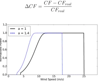
we use a location-adapted power curve, proposed by Jourdier [20]. In this
300
curve, the wind speed is divided by a location-dependent parameter a,
cho-301
sen so that the modified power curve has a capacity factor of 23% on the
302
calibration period. This corresponds to the average capacity factor in France
303
in 2014 [33]. This procedure is illustrated in Figure 8.
304
To assess the accuracy of the reconstructed capacity factor, the relative
305
error between the reconstructed capacity factor and the capacity factor from
306
the reanalysis is computed :
307
∆CF = CF − CFreal
CFreal
(12)
Figure 8: Example of the location-adapted power curve. In solid black: the real power curve for wind speed at 80m height; in dashed blue: the adapted power curve. It has the same shape, but the wind speed is divided by a number a to achieve a capacity factor of 23%.
Figures 9 and 10 show the relative error on the calculated capacity factor
308
for monthly and seasonal reconstructions respectively. At both timescales,
la
ti
tu
de
6.75°W 2.75°W 1.25°E 5.25°E 9.25°E 43.5°N
46.5°N 49.5°N
a
6.75°W 2.75°W 1.25°E 5.25°E 9.25°E 43.5°N
46.5°N 49.5°N
b
longitude
6.75°W 2.75°W 1.25°E 5.25°E 9.25°E 43.5°N 46.5°N 49.5°N c longitude la ti tu de
6.75°W 2.75°W 1.25°E 5.25°E 9.25°E 43.5°N
46.5°N 49.5°N
d
longitude
6.75°W 2.75°W 1.25°E 5.25°E 9.25°E 43.5°N 46.5°N 49.5°N e −100 −75 −50 −25 −10 −5 5 10 25 50 75 100 Re la ti ve e rr or o n C F (% )
Figure 9: Relative error on the capacity factor (%) for monthly distributions given by: non parametric climatology (a), parametric climatology (b), Wasp (c), Perc (d), and KCrec (e)
la
ti
tu
de
6.75°W 2.75°W 1.25°E 5.25°E 9.25°E 43.5°N
46.5°N 49.5°N
a
6.75°W 2.75°W 1.25°E 5.25°E 9.25°E 43.5°N
46.5°N 49.5°N
b
longitude
6.75°W 2.75°W 1.25°E 5.25°E 9.25°E 43.5°N 46.5°N 49.5°N c longitude la ti tu de
6.75°W 2.75°W 1.25°E 5.25°E 9.25°E 43.5°N
46.5°N 49.5°N
d
longitude
6.75°W 2.75°W 1.25°E 5.25°E 9.25°E 43.5°N 46.5°N 49.5°N e −100 −75 −50 −25 −10 −5 5 10 25 50 75 100 Re la ti ve e rr or o n C F (% )
the Perc method overestimates it mostly onshore by about 25% on average.
310
The KCrec method behaves like the Perc methods at the monthly scale, but
311
is performing better at the seasonal scale with an overestimation of about
312
10% onshore. As expected, the Wasp method shows good performance in
es-313
timating the capacity factor as its reconstruction focuses on the right tail of
314
the Weibull distribution. Nevertheless, it overestimates the energy
produc-315
tion in the northern part of France at a monthly scale and underestimates
316
it in the southern part of France at a seasonal scale. The non-parametric
317
climatology behaves very well at the seasonal scale even though it displays a
318
slight overestimation in the north of France. At the monthly scale, on
aver-319
age, on the entire domain it overestimates the capacity factor by about 25%.
320
By contrast, the parametric climatology behaves very badly at the monthly
321
scale, overestimating the energy production by 50% in average. At a seasonal
322
scale, this overestimation decreases but is still high, highlighting again the
323
error induced by the Weibull distribution hypothesis.
324
In any case, there is a tendency of all methods to overestimate the capacity
325
factor, mostly onshore. The climatology acts as a filter of high frequency
326
variation of the wind, meaning that it does not describes well the tails of
327
the distribution. As the power curve is designed so that the wind turbine
328
works at its nominal power near the mean wind speed, this results in an
329
overestimation of the capacity factor.
330
On the other hand, Drobinski et al. [21] showed that a Weibull
distri-331
bution fitted by MLE describes well the center of the distribution (near the
332
mean wind speed), but tends to underestimate the tails of the distribution.
333
This leads to the same consequence. That explains why the parametric
clima-334
tology acts worse than the non-parametric climatology, but also why KCrec
335
overestimates the capacity factor. This has no such effect offshore because
336
the wind above sea is steadier so that the distribution is more peaked around
337
the mean. Regarding the Perc method, the Weibull reconstruction is based
338
on two percentiles defined to minimize the CvM score. It may results in
339
the same effect of underestimation of the tails of the distribution. Future
340
work could focus on a sensitivity analysis to the percentiles definition by
341
minimizing the error on capacity factor.
342
At the seasonal scale, the real distribution is based on a larger sample
343
which implies that the center of the distribution has a much larger weight
344
than the tails at this scale than at the monthly scale. The effect of
underes-345
timating the tails is thus less visible.
4. Towards monthly and seasonal forecast of the wind speed
dis-347
tribution
348
The analysis described above has shown that the large-scale state of the
349
atmosphere contains information on the likely distribution of surface winds,
350
and our proposed methods allow to recover at least part of this information.
351
A long-term perspective will be to use this to build forecasts of surface wind
352
distributions. Below we present a preliminary attempt based on existing
353
seasonal forecasts, to assess the potential of this method for monthly or
354
seasonal forecasts.
355
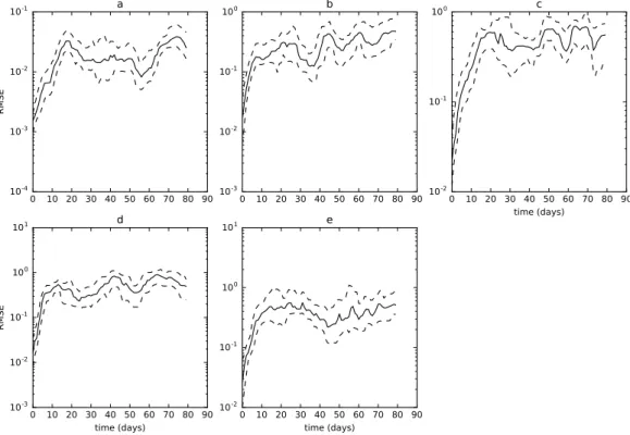
A first step is to assess the skill in seasonal forecasts for predicting the
356
large-scale state of the atmosphere in our region of interest. The root mean
357
square error (RMSE) between the daily PCs of Era-Interim and those of the
358
seasonal forecast is shown in Figure 11. This figure gives an idea of the
lead-359
time of such a forecast. It shows that the error increases rapidly until it levels
360
off after 20 days indicating that there is no more valuable information on the
361
large-scale circulation in the data. As a consequence, it will not be possible
362
to have an accurate wind distribution forecast at more than the monthly
363
horizon.
364
One technical difficulty arises: the monthly distribution of wind coming
365
from the ECMWF analysis stands for the real distribution. As the analysis
366
does not come from the same model as the ERA-Interim data, a bias
ex-367
ists between the distributions coming from the analysis and the distributions
368
based on ERA-Interim data. We thus apply a classical quantile/quantile
369
correction between the 4 years based distributions of the analysis and of
370
ERA-Interim between 2012 and 2015 at each point of the gridded domain.
371
We apply this correction to the monthly wind distribution of the analysis.
372
Because of the small amount of forecasts and of the uncertainties due to the
373
bias, we will not be able to have the same deep analysis as in the
reconstruc-374
tion part of the paper. The corrected monthly distribution of the wind speed
375
coming from the analysis is compared to the climatology of ERA-Interim and
376
to the forecast distributions using the CvM score.
377
The percentage of time each method does better than the climatology,
378
averaged over the entire domain, for the 1st month of the 12 forecasts, is
379
summarized in table 3. The results for the Perc and KCrec methods are
380
comparable to the reconstruction results. On the contrary, the Wasp method
381
shows a very high score when evaluating the entire distribution and a lesser
382
score when evaluating the energy production, which is not consistent with
0 10 20 30 40 50 60 70 80 90 10-4 10-3 10-2 10-1 RM SE a 0 10 20 30 40 50 60 70 80 90 10-3 10-2 10-1 100 b 0 10 20 30 40 50 60 70 80 90 time (days) 10-2 10-1 100 c 0 10 20 30 40 50 60 70 80 90 time (days) 10-3 10-2 10-1 100 101 RM SE d 0 10 20 30 40 50 60 70 80 90 time (days) 10-2 10-1 100 101 e
Figure 11: RMSE calculated between the PCs of Era-Interim and the PCs of the seasonal forecast. The solid line represents the median of the error, dashed lines represent the 60th percentile (top) and the 40th percentile (bottom). a. Seasonal, b. NAO, c. EA, d. SCA, e. EU2
Forecast method Wasp Perc KCrec
total 1st month 46.4 (31.2 ) 20.2 (25.5 ) 28.8 (27.5 ) 2012 41.0 (35.0 ) 15.1 (20.5 ) 22.9 (23.6 ) 2013 44.1 (25.7 ) 22.9 (25.4 ) 32.4 (26.5 ) 2014 54.0 (33.0 ) 22.5 (30.4 ) 31.3 (32.3 )
Table 3: Percentage of the number of times each method does better than the climatology on the whole domain for the 3 years of forecasts. First values correspond to the evalua-tion of the entire distribuevalua-tion; values in parenthesis corresponds to the evaluaevalua-tion of the distribution between the cut in and the cut out.
the reconstruction results. When calculating the error on the capacity factor,
384
the forecast methods always highly overestimate the wind energy production
385
onshore (more than 100% at some points), and slightly underestimate it
off-386
shore (more than 10%). The non-parametric climatology overestimates the
capacity factor by more than 10% onshore and underestimates it offshore,
388
whereas the parametric climatology highly overestimates the energy
produc-389
tion on the whole domain as it was the case in the evaluation part.
390
Regarding the large uncertainty due to the limited number of forecasts,
391
the robustness can be inferred from the consistency of the forecasts results
392
with those obtained in the previous section.
393
Still, work must be continued to evaluate the forecasts performance of
394
such methods, by using larger sets of numerical seasonal weather forecast,
395
but also by testing methods based on non-parametric distribution estimation.
396
5. Conclusion
397
In this paper, a new approach for modelling the wind speed at the seasonal
398
scale has been proposed. We suggest to model not only the mean wind speed
399
but the entire monthly/seasonal distribution of the wind. Linking the wind to
400
its synoptic predictors we have shown that there is valuable information in the
401
large-scale circulation variability that can explain the wind speed distribution
402
at such long timescales. The proposed methods show good performances in
403
reconstructing the monthly and seasonal wind speed distributions even if
404
the climatology is still a good predictor. Moreover, reconstruction methods
405
performances display an interesting spatial and seasonal variability. Indeed,
406
in the north of France in winter and fall, the proposed methods showed
407
better ability to model strong winds than the climatology. Nevertheless,
408
the attempt of forecasting also highlights the fact that seasonal forecasts of
409
ECMWF are not yet mature enough to give valuable information on the
410
large-scale circulation variability at the horizons exceeding a month.
411
Acknowledgments
412
This research was supported by the ANR project FOREWER
(ANR-14-413
CE05- 0028). This work also contributes to the HyMeX program
(HYdro-414
logical cycle in The Mediterranean EXperiment [34]) through the working
415
group Renewable Energy.
Appendix: Cramer-Von Mises score
417
To assess the reconstruction quality, we use the Cramer-Von-Mises score
418
defined in Anderson et al. [35]:
419 CvM = M N M + N ∫ ∞ ∞ [FN(x)− FM(x)]2dHM +N(x) (.1)
Here, M and N are the sample sizes in each of the distributions, FN(x)
420
and FM(x) are the CDFs of the two samples and HM +N(x) is the combined
421
distribution of the two samples together. The smaller the CvM score, the
422
better the goodness of fit between the two tested distributions. Anderson et
423
al. [35] showed that Equation (.1) is equivalent to
424
CvM = U
N M (M + N ) −
4N M− 1
6(N + M), (.2)
where U = N∑Ni=1(ri−i)2+M
∑M
j=1(rj−j)2, riare the ranks of the elements
425
of the sample of size N in the combined sample and rj are the ranks of the
426
sample of size M in the combined sample.
427
The CvM score allows to test the null hypothesis H0:”the two samples
428
come from the same distribution”. When M→∞ and N→∞, under the null
429
hypothesis, the CvM score follows the limiting distribution with mean 16 and
430
variance 451. In this configuration, the p-value giving 95% confidence that
431
the null hypothesis is true is p = 0.46136, [35].
432
References
433
[1] EWEA, Wind in power: 2014 European statistics, European Wind
En-434
ergy Association.
435
[2] S. S. Soman, H. Zareipour, O. Malik, P. Mandal, A review of wind power
436
and wind speed forecasting methods with different time horizons, North
437
American Power Symposium (NAPS) (2010) 1–8.
438
[3] W. Chang, A literature review of wind forecasting methods, Journal of
439
Power and Energy Engineering 2 (2014) 161–168.
440
[4] A. Sfetsos, A novel approach for the forecasting of mean hourly wind
441
speed time series, Renewable Energy, 27 (2002) 163–174.
[5] P. Gomes, R. Castro, Wind speed and wind speed forecasting using
sta-443
tistical models: Autoregressive Moving Average (ARMA) and Artificial
444
Neural Networks (ANN), International Journal of Sustainable Energy
445
Development (IJSED) 1.
446
[6] A. Carpinone, M. Giorgio, R. Langella, A. Testa, Markov chain
model-447
ing for very-short-term wind power forecasting, Electric Power Systems
448
Research 122 (2015) 152 – 158.
449
[7] J. Taylor, P. McScharry, R. Buizza, Wind power density forecasting
450
using ensemble prediction and time series model, IEEE Transactions on
451
Energy Conversion 34.
452
[8] M. Wytock, J. Z. Kolter, Large-scale probabilistic forecasting in energy
453
systems using sparse gaussian conditional random fields, Proceedings of
454
the IEEE Conference on Decision and Control (2013) 1019–1024.
455
[9] T. G. Barbounis, J. B. Theocharis, M. C. Alexiadis, P. S. Dokopoulos,
456
Long-termwind speed and power forecasting using local recurrent neural
457
network models, IEEE Transaction on Energy Conversion 21 (2006) 273–
458
284.
459
[10] J. Najac, J. Boe, L. Terray, A multi model ensemble approach for
as-460
sessment of climate change impact on surface winds in France, Climate
461
Dynamics 32 (2009) 615–634.
462
[11] D. J. Sailor, M. Smith, M. Hart, Climate change implications for wind
463
power resources in the northwest united states, Renewable Energy 33
464
(2008) 23932406.
465
[12] S. Pryor, R. Barthelmie, Climate change impacts on wind energy: A
466
review, Renewable and Sustainable Energy Reviews 14 (2010) 430437.
467
[13] M. Bilgili, B. Sahin, A. Yasar, Application of artificial neural networks
468
for the wind speed prediction of target station using reference stations
469
data, Renewable Energy 32 (2007) 2350–2360.
470
[14] H. B. Azad, S. Mekhilef, V. G. Ganapathy, Long-term wind speed
fore-471
casting and general pattern recognition using neural networks, IEEE
472
Transaction on Sustainable Energy 5 (2014) 546553.
[15] J. Wang, S. Qin, Q. Zhou, H. Jiang, Medium-term wind speeds
forecast-474
ing utilizing hybrid models for three different sites in xinjiang, china,
475
Renewable Energy 76 (2015) 91–101.
476
[16] Z. Guo, W. Zhao, H.Lu, J.Wang, Multi step forecasting for wind speed
477
using a modified EMD based artificial neural network model, Renewable
478
Energy 37 (2012) 241–249.
479
[17] A. More, M. Deo, Forecasting wind with neural networks, Marine
Struc-480
tures 16 (2003) 35–49.
481
[18] J. Owen, T. Palmer, The impact of El Nino on an ensemble of extended
482
range forecasts, American Meteorological Society 115 (1987) 2103–2117.
483
[19] C. Cassou, Intraseasonal interaction between Madden-Julian oscillation
484
and the North Atlantic Oscillation, Nature 455 (2008) 523–597.
485
[20] B. Jourdier, Wind resource in metropolitan france: assessment methods,
486
variability and trends, Ph.D. thesis, Ecole Polytechnique (2015).
487
[21] P. Drobinski, C. COulais, B. Jourdier, Surface wind-speed statistic
mod-488
elling: Alternatives to the Weibull distribution and performance
evalu-489
ation, Boundary-Layer Meteorol 157 (2015) 97123.
490
[22] D. P. Dee, S. M. Uppala, A. J. Simmons, P. Berrisford, P. Poli,
491
S. Kobayashi, U. Andrae, M. A. Balmaseda, G. Balsamo, P. Bauer,
492
P. Bechtold, A. C. M. Beljaars, L. van de Berg, J. Bidlot, N. Bormann,
493
C. Delsol, R. Dragani, M. Fuentes, A. J. Geer, L. Haimberger, S. B.
494
Healy, H. Hersbach, E. V. Holm, L. Isaksen, P. Kallberg, M. Kohler,
495
M. Matricardi, A. P. McNally, B. M. Monge-Sanz, J.-J. Morcrette, B.-K.
496
Park, C. Peubey, P. de Rosnay, C. Tavolato, J.-N. Thepaut, F. Vitart,
497
The era-interim reanalysis: conguration and performance of the data
498
assimilation system, Q. J. R. Meteorol. Soc. 137 (2011) 553597.
499
[23] F. Molteni, T. Stockdale, M. Balmaseda, G. Balsamo, R. Buizza, L.
Fer-500
ranti, L. Magnusson, K. Mogensen, T. Palmer, F. Vitart, The new ecmwf
501
seasonal forecast system (system 4), ECMWF Technical Memorandum
502
656.
503
[24] T.Burton, N.Jenkins, D. Sharpe, E. Bossanyi, Wind energy handbook,
504
Wiley.
[25] J. Manwell, J. McGowan, , A. Rogers, Wind energy explainded. theory,
506
design and application, Wiley.
507
[26] M. Vrac, P. V. Ayar, P. Yiou, Trends and variability of seasonal weather
508
regimes, International Journal of Climatology.
509
[27] C. Cassou, L. Terray, J. W. Hurrel, C. Deser, North atlantic winter
510
climate regimes: Spatial asymmetry, stationarity with time, and oceanic
511
forcing, American Meteorological Society.
512
[28] I. Lun, J. Lam, A study of Weibull parameters using long-term wind
513
observation, Renewable Energy 20 (2000) 145–153.
514
[29] C. Justus, W. Hargreaves, A.Yalcin, Nationwide assessment of potential
515
output from wind-powered generators, Journal of Applied Meteorology
516
15 (1976) 673–678.
517
[30] I. T. N.G. Mortensen, L. Landberg, E. Petersen, Wind atlas analysis
518
and application program (wasp), vol.1: Getting started. vol.2: Users
519
guide., Ris National Laboratory.
520
[31] S. Pryor, M. Nielsen, R. Barthelme, J.Mann, Can satellite sampling
521
of offshore wind speeds realistically represent wind speed distributions?
522
Part II: Quantifying uncertainties associated with distribution fitting
523
methods, American Meteorological Society.
524
[32] A. Cohen, Maximum likelihood estimation in the Weibull distribution
525
based on complete and censored samples, Technometrics 7 (1965) 579–
526
588.
527
[33] RTE, Syndicat des Energies Renouvelables, ERDF and ADEef,
528
Panorama de l’electricite renouvelable 2014.
529
[34] P. Drobinski, V. Ducrocq, P. Alpert, E. Anagnostou, K. Branger,
530
M. Borga, I. Braud, A. Chanzy, S. Davolio, G. Delrieu, C. Estournel,
531
N. F. Boubrahmi, J. Font, V. Grubisic, S. Gualdi, V. Homar, B.
Ivancan-532
Picek, C. Kottmeier, V. Kotroni, K. Lagouvardos, P. Lionello, M. Llasat,
533
W. Ludwig, C. Lutoff, A. Mariotti, E. Richard, R. Romero, R. Rotunno,
534
O. Roussot, I. Ruin, S. Somot, I. Taupier-Letage, J. Tintore, R.
Uijlen-535
hoet, H.Wernli, A 10-year multidisciplinary program on the
Mediter-536
ranean water cycle, Meteorol. Soc. 95 (2014) 1063–1082.
[35] T. Anderson, On the distribution of two sample Cramer Von Mises
538
criterion, The Annals of Mathematical Statistics (1962) 1148–1159.