HAL Id: halshs-01122659
https://halshs.archives-ouvertes.fr/halshs-01122659
Preprint submitted on 4 Mar 2015
HAL is a multi-disciplinary open access
archive for the deposit and dissemination of sci-entific research documents, whether they are pub-lished or not. The documents may come from teaching and research institutions in France or abroad, or from public or private research centers.
L’archive ouverte pluridisciplinaire HAL, est destinée au dépôt et à la diffusion de documents scientifiques de niveau recherche, publiés ou non, émanant des établissements d’enseignement et de recherche français ou étrangers, des laboratoires publics ou privés.
Greenfield versus Merger & Acquisition FDI: Same
Wine, Different Bottles?
Ronald B. Davies, Rodolphe Desbordes, Anna Ray
To cite this version:
Ronald B. Davies, Rodolphe Desbordes, Anna Ray. Greenfield versus Merger & Acquisition FDI: Same Wine, Different Bottles?. 2015. �halshs-01122659�
Greenfield versus Merger & Acquisition FDI:
Same Wine, Different Bottles?
Ronald B. DAVIES
Univ. College Dublin
Rodolphe DESBORDES
University Strathclyde
Anna RAY
Paris School of Economics Sciences Po. and Paris 1
March 2015
G-MonD
Working Paper n°39
Greenfield versus Merger & Acquisition FDI:
Same Wine, Different Bottles?
∗
Ronald B. Davies
†Rodolphe Desbordes
‡Anna Ray
§Abstract
Relying on a large foreign direct investment (FDI) transaction level dataset, unique both in terms of disaggregation and time and country coverage, this paper examines patterns in greenfield (GF) versus merger & acquisition (MA) investment. Although both are found to seek out large markets with low international barriers, important dif-ferences emerge. MA is more affected by geographic and cultural barriers and exhibits opportunistic behaviours as it is more sensitive to short-run changes, such as a currency crisis. On the other hand, GF is relatively driven by long-run factors, such as origin-country technological and institutional development or comparative advantage. These empirical facts are consistent with the conceptual distinction made between these two modes, i.e. MA involves transfer of ownership for integration or arbitrage reasons while GF relies on firms own capacities, which are linked to the origin countries attributes. They also suggest that GF and MA are likely to respond differently to policies intended to attract FDI.
Keywords: Foreign Direct Investment; Mergers and Acquisitions; Greenfield Invest-ment; Multinational Firms
JEL Classification: F21; F23
∗We thank Matthieu Crozet and Farid Toubal for helpful comments. All errors are our own. †University College Dublin. [email protected]
‡University Strathclyde [email protected]
§Sciences Po, Paris School of Economics and Universit´e Paris 1 Pant´eon-Sorbonne. anna.ray@
1
Introduction
Foreign direct investment (FDI) occurs via two modes, greenfield (GF) investment and cross-border mergers and acquisitions (MA). The implicit distinction between the two modes is that GF investment relies on the internal capabilities of the multinational enterprise (MNE), as is most clearly embodied in the notion of building a new subsidiary from the ground up; MA meanwhile involves transfer of ownership of an existing asset. Although there is widespread recognition of the distinct nature of these modes, due to data constraints there is little research actually comparing GF and MA FDI. Further, what does exist almost exclusively relies on data for a single developed country. In addition, while it is generally presumed that most worldwide FDI flows are MA (e.g. Globerman and Shapiro, 2004 or Head and Ries, 2008), these statements rely on data during the 1990s and miss the remarkable growth of primarily GF FDI in developing countries during the 2000s (UNCTAD, 2014). Thus, there is a need for a study comparing GF and MA FDI using more recent data. This paper fulfills that need by using a unique combined transaction-level dataset covering worldwide GF and MA FDI for the period 2003-2010 across 37 manufacturing and services sectors. This level of disaggregation has been heretofore unavailable and allows us to compare not only the developed and developing country experiences but also the sectoral composition of FDI modes.
We find that the two modes share several similarities. For example, both tend to come from the developed countries and are affected by traditional “gravity” variables such as GDP and distance. Similarly, both are dominated by manufacturing, although services form a significant share of overall FDI flows and comprise the largest sectors within each mode. Nevertheless, there are key differences across modes. While the developed countries receive the majority of MAs, developing countries host the bulk of GF FDI. In addition, our count data regression analysis shows that MA investment is more responsive to barriers between the origin and destination countries, including investment cost and geographical and cultural barriers. MA also features more opportunistic behaviour in that it is more sensitive to
short-run variations such as changes in market size, changes in capital market depth, or a currency crisis. In contrast, GF is far more sensitive to long-run factors, targeting more low-tax locations and relying more on home technological development, quality of institutions, and the degree of comparative advantage. These results are on the whole consistent with the conceptual distinction made between the two modes; namely, that MA involves transfer of ownership (arising from a desire to integrate or exploit arbitrage opportunities) whereas GF relies more on a firm’s own capacities (which are intrinsically linked to the origin country’s attributes).
An important aspect of our data is that unlike other studies, we can compare FDI between developed countries (which dominates the data) with that going to and/or coming from the South. Doing so is important because MA FDI is skewed towards developed countries whereas GF is the opposite. Indeed, we find that differences between modes with respect to variables such as distance between countries is in part driven by the different geographic concentrations of the two modes of FDI. Similarly, by exploiting our sector data, we are able to identify how differences between modes vary by industry. For example, although manufacturing GF is less responsive to a common language than its MA counterpart, in services, the two modes respond equally to a shared language.
Recognizing these differences is important to understanding the patterns of FDI and therefore the policies that can be used to attract one type of investment relative to another. This matters since the potential impacts of FDI can vary by mode. For example, as discussed by Davies and Desbordes (forthcoming), outbound GF may have much stronger negative effects on an origin country’s labour market than does MA. Thus, if a country experiences FDI outflows due to falling tax rates elsewhere, our estimates suggest this would primarily be in GF and therefore have larger than average labour market effects.
The paper proceeds as follows. First, we review the existing literature on FDI with a focus on that comparing the two modes of investment. Section 3 describes our data. Section 4 contains a set of stylized facts for the two modes, including a discussion of the primary
origins, destinations, and sectors for MA and GF FDI. Section 5 expands on these stylized facts by utilizing regression analysis to estimate where the two modes move in similar - and in different - ways in response to origin, destination, and country pair characteristics. Section 6 concludes.
2
The Literature on FDI Mode
The literature on FDI is vast, covering models suggesting why FDI occurs, empirical studies testing those models, analyses of the impacts of FDI, and suggestions on the management of MNEs via government policy.1 Despite this plethora of papers, there is remarkably little discussing both GF and MA FDI, either theoretically or empirically.2 In this section, we
describe this small body of research.
The theory on mode choice typically starts at the firm level, where an individual firm chooses its entry mode accounting for the costs and benefits of each, a decision which can then be included in a general equilibrium model. A prime example of this approach is Nocke and Yeaple (2008) who provide a model in which a MNE establishes a subsidiary for two reasons: lowering production costs and hiring new entrepreneurs who provide headquarter services. While both modes seek lower production costs, only MA acquire new entrepreneurs by purchasing an acquisition target whereas GF makes do with those it has in the origin country.3 An implication of this is that, since a new entrepreneur is only beneficial to the firm
if her productivity exceeds that of the origin-country entrepreneur, firms with high origin 1For brevity, we do not attempt to provide a comprehensive overview of the FDI literature and focus
only on what is most relevant to the comparison between GF and MA. See Navaretti and Venables (2006), Blonigen (2005), and Blonigen and Piger (2011) for recent overviews of the broader literature on FDI.
2There are, however, many papers discussing one mode or the other. Examples of GF models include
Helpman (1984), Markusen (1984), and Helpman et al. (2004). Neary (2007) and Head and Ries (2008) provide models where FDI is exclusively MA.
3For evidence on the choice of target, see Blonigen et al. (2012), and Guadalupe et al. (2012) who focus
on the characteristics of the target (so called “cherry picking”). Herger and McCorriston (2014) analyze the linkages between the acquired and target firm via input-output tables, finding a large role for vertical acquisitions and a surprisingly large share of acquisitions for which there are no obvious industrial linkages. Ray (2014) compares the acquirer and target in product space. She shows that even in the absence of direct linkages, multinationals acquire activities in industries relatively closely related to their own spectrum of products.
productivity are unlikely to gain from MA and therefore focus on GF.4 In addition, due to
complementarities between production and headquarter services, productive firms (and thus GF firms) will dominate when there are large production cost differences (such as between the developed North and less-developed South). On the other hand, North-North FDI will be predominantly MA. Finally, the tradeoff between modes depends on their relative costs. When targets in the destination are scarce, making MA costly, GF will naturally dominate. Conversely, if the establishment of a GF subsidiary is more difficult, MA will dominate. The authors then confirm these patterns using aggregated US outbound FDI.
A concurrent set of theories focuses on the price of MA as a crucial component in the choice of whether to choose GF or MA. For example, Raff et al. (2009) provide a model where the acquisition price is forward looking, i.e. where the potential target recognizes that, should they charge a high acquisition price, this can lead to GF investment which increases the number of firms and has consequences for their profits.5 Muller (2007) provides a model
in which changes in competition feed into the acquisition price and shows that it depends on the extent of existing competition in the country. In particular, GF FDI will be preferred when there are either few or many firms; MA FDI will dominate under moderate competition. Note that in contrast to Nocke and Yeaple (2008), the tradeoff in this line of research is less about the transfer or acquisition of technology but more about changes in competition.
The empirical work on mode choice also has two main themes. The first looks at the choice of mode for a given firm using a discrete dependent variable methodology. For example, Drogendijk and Slangen (2006) use survey data from Dutch MNEs to focus on the role of cultural distance in the mode choice, finding that greater cultural barriers tend to encourage GF over MA. Other examples can be found in the survey of the business literature provided by Slangen and Hennar (2007). As they discuss, of the results that are consistent across studies, MA dominate in wealthier targets (consistent with Nocke and Yeaple, 2008) whereas 4In a related paper Nocke and Yeaple (2007) show that this productivity ranking, and hence the impact of
country characteristics, can depend on whether the firm productivity differences relates to the international mobility of its production characteristics.
GF dominates when cultural differences are large. A difficulty with all of this work, however, is that these studies typically only use data on the outbound FDI of a single country (with the exceptions being data on inbound FDI to a single destination or for a very small number of countries). As suggested by Slangen and Hennar (2007), this, along with the lack of a consistent set of regressors across studies, may drive the general lack of consistent findings. The second strand of empirical literature uses aggregated FDI (typically at the country level). Perhaps the most utilized data for this is that provided by UNCTAD (2014), which produces annual reports documenting the world-wide and regional patterns of GF and MA FDI. Using these data in a cross-section, Globerman and Shapiro (2004) compare how FDI inflows and outflows vary with gravity variables (measures of market size and trade and investment costs) for both the full and MA only samples.6 They find that all FDI is attracted
to larger economies, with MA particularly so. In addition, drawing from the literature looking exclusively at MA FDI, they control for a variety of institutional and financial depth measures, again finding that MA is typically more sensitive to these factors than is overall FDI.7 Neto et al. (2009) extend this analysis to a panel and include cultural variables,
finding that they appear to be more important for GF than MA.8 Park et al. (2012) also make use of the UNCTAD data, restricting themselves to the developing countries and employing alternative estimating techniques, resulting in comparable findings. These studies are limited, however, by their lack of bilateral FDI information, making them unable to estimate the role of key gravity variables such as the distance between origin and destination or shared languages. In addition, depending on the year, UNCTAD provides multilateral data on aggregate FDI and MA (number of projects and total value), but the GF data
6See Blonigen and Piger (2011) for an overview of the standard gravity controls in FDI regressions. 7Examples of studies looking at the effect of institutions and/or financial depth on MA FDI include Rossi
and Volpin (2004), di Giovanni (2005), Hyun and Kim (2007), Hur et al. (2011), and Coeurdacier et al. (2009). Desbordes and Wei (2014), using data on GF flows, find that both origin and destination financial development are driving factors.
8DiGuardo et al. (2013) also find that physical, cultural and political distances reduce MA flows but
do not consider GF flows. Azemar et al. (2012) point to market familiarity (a combination bilateral ties, experience with weak institutions, and lack of international experience) as an important factor in FDI between developing countries.
only becomes available in 2002. Hence in Park et al. (2012), the GF data are created by subtracting MA flows from aggregate FDI.9 As this ignores other possible forms of FDI changes, such as equity increases by existing projects via retained earnings, non-standardized reporting definitions and reporting across countries, and round-tripping FDI, this is not a clear-cut comparison between MA and GF FDI.
Despite the advantages in using bilateral data, there is very little work exploiting it. Hebous et al. (2011) have bilateral data decomposing FDI into GF and MA for outbound German investments. This allows them to include both distance, which impedes GF less than MA (in contrast to Nocke and Yeaple, 2008), and the tax rate of the destination, finding that MA is less sensitive to destination taxes than is GF. In her comparison of GF and MA FDI across US states, Swenson (2001) finds a similar difference in tax sensitivities. These results are consistent with the model of Becker and Fuest (2010), who indicate that tax advantages of a particular destination are likely to be capitalized into the acquisition price, something which would not happen with GF. Outside of these tax-oriented studies, in a comparison between MA flows and total FDI flows (a comparison which is subject to the same caveats as in the above work using the aggregate UNCTAD data), Klein and Rosengren (1994) find that inbound US MA investments are marginally more sensitive to exchange rate variation than are aggregate flows. This then lends support to the notion of “fire sale” FDI, that is, investments which are spurred by a decline in the cost of establishing/acquiring the affiliate due to exchange rate movements (Froot and Stein, 1991).10
Combining the above results, several overarching predictions emerge. First, we would expect the levels of both GF and MA to respond in comparable ways to the traditional gravity variables, i.e. levels of FDI are greater between large, wealthy countries with small barriers between them. Second, in line with Nocke and Yeaple (2008) we anticipate that 9Neto et al. (2009) on the other hand combine MA data in values for 1996-2002 with GF data with
number of projects for 2002-2006.
10In this type of investment, coined by Krugman (2000), the firm’s intent is more driven by the ability to
acquire a investment asset while its price is low rather than the traditional motives ascribed to MA FDI. Evidence of such behavior is found by Blonigen (1997). See also Aguiar and Gopinath (2005).
MA (which generally originates in income countries) is particularly drawn to high-income countries, both due to the availability of potential targets as well as the assignment predictions of their model. Third, we anticipate that MA is relatively more sensitive to destination financial depth and institutional quality. Fourth, we anticipate that distances, be they cultural or physical, impact GF less than MA investments. Finally, we expect that GF is more sensitive to destination taxes whereas MA is more responsive to exchange rate shocks.
3
Data Description
In this section, we discuss our variables of interest, which measure GF and MA FDI, as well as the control variables we use in our regression analysis. Our key variables are F DIm,o,d,s,t
which is the number projects via FDI mode m from origin country o to destination d in sector s in year t. In order to simplify our discussion, we use the term project to mean an investment project, that is a GF investment or a MA. The mode of the project refers to whether it is GF, i.e. a new project that did not exist before, or MA, that is the merger with or acquisition of a pre-existing entity. The list of the 39 sectors in our study is in Table 1. While our sample covers the globe, in our discussion and tables we refer to specific countries. The list of country abbreviations used is found in Table 2.
3.1
Construction of GF
Our GF data come from fDi Markets, which is a commercial database tracking the universe of cross-border greenfield investments that covers all sectors and countries worldwide since 2003.11 The data are available at the project level, that is, an individual GF investment. These data report the source and destination countries as well as the sector of the GF project 11This is the source of greenfield FDI data for the UNCTAD (2014) data. It can be found at http:
(note that this is the sector of the project, not the parent firm undertaking the project).12
This classification is that in Table 1. Unfortunately, it does not report a measure of the size of the investment which is comparable to those in the MA data. Further, it does not provide us detailed information on the parent firm. Thus, we cannot utilize the data for a meaningful study at the observation level `a la Drogendijk and Slangen (2006) and instead aggregate these up to the origin, destination, sector, year level, making our data more similar to that of Hebous et al. (2011). Finally, note that these projects can represent either a new GF project in a destination country where the source firm was already active or a first time entry into a destination.
3.2
Construction of MA
These data come from the Zephyr database, produced by Bureau van Dijk from press re-leases.13 Zephyr claims to cover the universe of domestic and international MA projects across the globe with a value above 1 million British pounds.14 Although the data begin in 2000 (and extend back to 1997 for the USA and European countries), here we utilize only the data since 2003 to match the GF data. As with the GF data, these are at the project level. Although there is more detailed information on both the acquiring firm (located in the origin) and the target (located in the destination), without comparable information in the GF data, these are of little use in our comparisons. In order to match the GF information, we therefore aggregated up to the source, destination, sector, year level. In doing so, there were two challenges.
First, the MA data report both a country name and a country code for the source and destination. While in most cases the name and code match, there are exceptions.15 In
these cases, we used the country code to allocate a project to a particular source/destination 12As we do not have data on the sector of the parent, we cannot identify vertical versus horizontal
investments as Herger and McCorriston (2014) do for MA data.
13These can be found at http://www.bvdinfo.com.
14Note that there is no comparable size threshold in the GF data.
15In the source data, mismatches were approximately 6% of projects. For destinations, the mismatch was
country. In other cases, only the name or the code was reported. In this situation, we used the available information to allocate the project. Finally, there were cases where neither the name nor the code was reported.16 In these cases, we allocated the project to a catch-all category (“Earth”) and these projects were then used in the below analysis when possible (i.e. when source was missing, we were still able to use the projects when considering destinations). We note this because in the analysis below utilizing source, destination, or source-destination pair information, these observations could not be used.
Second, unlike the GF data, the MA sectors are classified in 4-digit SIC codes, distin-guishing between codes of the parent and target firms. To correspond to the GF data, we used the target industry code as the code of the project and a correspondence from fDi
Mar-kets that maps SIC codes into the GF sector classification. However, this correspondence did
not cover all SIC codes. For some, we allocated the project by matching the SIC industry’s description and the GF sector description.17 Nevertheless, for about 6% of projects, there
was no clear-cut classification. Furthermore, the industry code was not reported for 18% of projects. These were allocated to a catch-all sector “Miscellaneous” for which there is no GF counterpart.
Finally, following the international standard, we included MA where a foreign firm ac-quired a minimum of a 10% stake in the affiliate. This 10% cutoff is common across countries in determining whether or not a foreign person has control, i.e. whether it counts as FDI.
3.3
Interpretation of the measures
Before continuing to a detailed analysis of the data, it is important to recognize what these GF and MA measures do and do not capture. These variables measure the number of new projects occurring between two countries in a given sector in a given year. As such, they are flow variable, not a measure of the stock of projects. Because of this, countries that feature 16These missing information cases amounted to 15.6% for the source data and 3.5% for the destination
data.
heavily in flows during the sample period (such as China) may still lag behind in their share of accumulated investment flows. In addition, these count investments, not dis-investments, meaning that they do not measure the net flows of projects. Furthermore, we focus here exclusively on FDI which is by definition cross-border investment and do not include what happens within a country. Thus, one must keep these issues in mind when interpreting the patterns and findings below. Finally, these data are count data and do not control for the size of the project (be that measured as employment, the value of investment, sales, or some other measure). We are forced to do this as there does not exist a comparable measure of size in the GF and MA datasets. Nevertheless, we endeavor to link these count measures back to the value of capital flows below.
3.4
Control variables
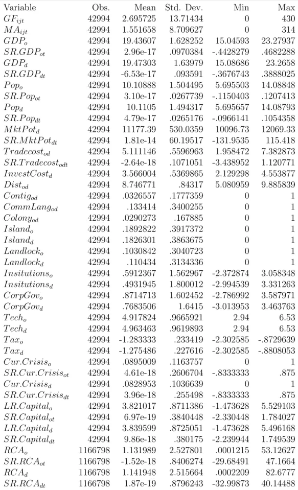
In our regressions, we utilize a set of canonical control variables which are standard in FDI analysis, including origin, destination, and pair-wise factors. Details on data sources, mea-surements, and summary statistics are in the Appendix. Broadly speaking, these “gravity” variables fall into two categories: market size and international barriers. For both the origin and destinations, we use GDP and population as measures of market size. Note that as both are in logs, including both implicitly controls for per-capita income. In addition, we include the destination’s market potential which is intended to control for the destinations proximity to other markets.18 For international barriers, we include a number of different measures. The first is the World Bank’s (2014) bilateral trade cost measure which controls for the ease of trade between the origin and destination. In addition, we use several geographic measures: the distance between them, a dummy equalling one when they are contiguous (i.e. share a common border), and dummy variables indicating whether the origin or destination is an island or landlocked country. To control for cultural differences, we include a dummy equal to one when the two countries share a common language and dummy indicating whether or
not they share a colonial history. As another measure of barriers, we include a proxy for destination investment costs.
Beyond these gravity variables, we utilize several measures of the political and economic environments. For both the origin and destination, we include proxies for institutional development, the quality of corporate governance, and to proxy for financial depth, the extent of stock market capitalization. In addition, to examine how FDI may be affected by exchange rate shocks, we include controls for whether or not the origin or destination country is experiencing a currency crisis. Given the importance attributed to destination taxes when making location decisions, we include the destination’s statutory corporate tax rate.19 Finally, as factor price differences potentially influential for mode choice (Nocke and Yeaple, 2008), we use the Balassa (1964) measure of revealed comparative advantage (RCA). This measure identifies a comparative advantage in a sector s for country i if the s’s share in i’s export basket exceeds s’s share in worldwide exports. Note that unlike our other measures, RCA is available at the sector level, however due to trade data limitations, we were only able to obtain measures for 28 of our sectors, most of which were in manufacturing. This list of sectors for which RCA is available is in Table 1.
4
Stylized Facts
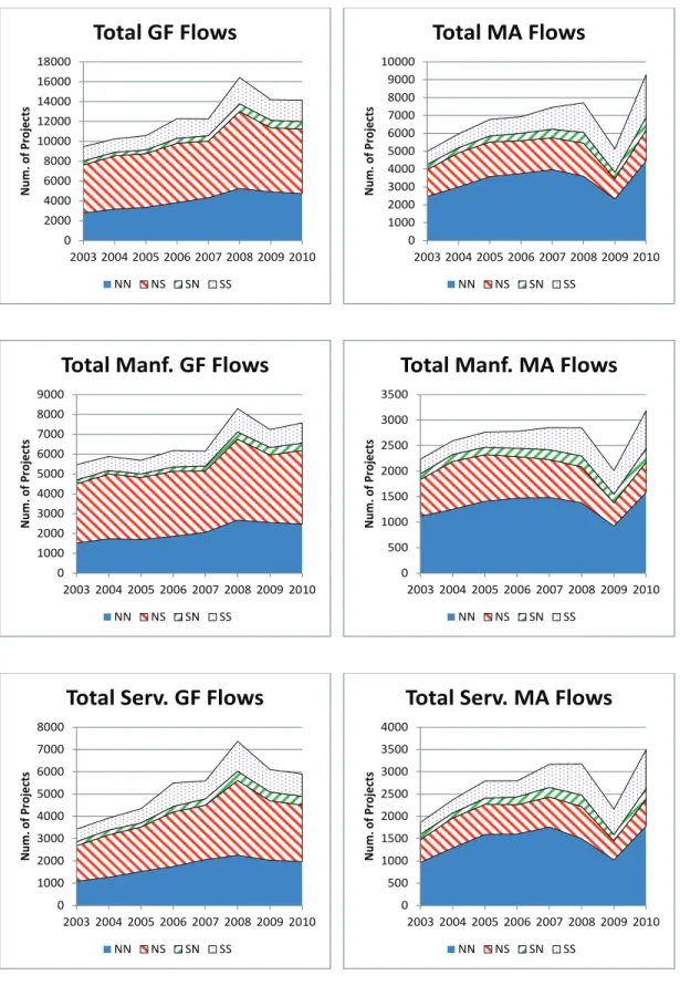
Before delving into the econometric analysis, it is beneficial to explore the data using simple descriptive statistics and construct a set of stylized facts regarding the overarching patterns in GF and MA flows. As stressed above, on the whole the two modes are often found to behave similarly, however, even a basic analysis reveals important differences. Figure 1’s top panel shows the evolution of GF and MA FDI over our sample period (for the moment, simply focus on the cumulated levels). From this, three key observations can be drawn. First, in terms of the number of projects, GF outstrips MA by nearly 50% (more on this 19Although the effective average tax rate would be more appropriate when estimating the decision of
below), with a total of 67,702 MA projects and 99,524 GF projects worldwide during our sample. Second, both have been generally growing during the sample period. Third, in response to the financial crisis of 2008-2009, both modes of FDI fell. This decline, however, was much more severe for MA. On the other hand, MA flows recovered to their pre-crisis levels by 2010 whereas GF flows remained stagnant.
Stylized Fact 1. GF accounts for roughly two-thirds of FDI activity. MA FDI fell more sharply following the financial crisis, but also recovered more quickly.
4.1
Top Origins and Destinations
Table 3 presents the top ten origins, destinations, and origin-destination pairs in terms of number of GF and MA projects. The most obvious feature of the origin and destination columns is in their overlap. The same seven countries are top origins for both GF and MA. Further, all the top origin and destination countries are developed Northern economies and, as a group, these ten nations generate a very large share of FDI, accounting for 49.7% and 68.7% of the total MA and GF projects in the sample. Overall, of the 264 countries in the worldwide sample, 64 are never origins for either mode with an additional 30 only being origins for MA. Turning to the destinations, we see a similar degree of overlap between the MA and GF countries. MA destinations are again predominantly developed (and indeed are also typically major sources of MA flows), with China being the exception. GF recipients, on the other hand, are more varied, with China, Russia, India and the United Arab Emirates ranking in the top ten. As with outflows, the top ten again account for roughly half of FDI inflows, although the GF inflows are noticeably less concentrated.
With respect to the country-pair ranking, the English speaking countries of the US, Canada, and the UK dominate the MA results. In addition, China is a major destination, particularly from other Asian locations and the US. Indeed, Japanese FDI in China has received a good deal of attention (e.g. Armstrong, 2009) and Singapore is well known financial hub that acts as an intermediary between China and the West. GF, however,
is again more varied. Although the Anglo-Saxon countries still feature heavily as origins, Japan is a primary source twice, whereas the destination countries cover both the major developed economies as well as large developing nations. Finally, it is worth recognizing the concentration in FDI flows, with these ten country pairs alone making up 14% of MA and 15% of GF FDI. Of the 59,782 possible country pairs, 53,792 never experience FDI of either mode, 1090 only see MA, and 2522 only see GF.
Stylized Fact 2. GF and MA FDI outflows are very concentrated among Northern economies. MA inflows are dominated by Northern countries; GF inflows are split between Northern and Southern countries. At the bilateral level, MA flows are dominated by Anglo-Saxon coun-try pairs and East-Asian flows towards China. GF flows, by comparison, are widely varied both in terms of origin and destination. In all cases, however, a small number of countries account for a large share of overall activity.
Thus, just as Nocke and Yeaple (2008) predict, Table 3 suggests that the mode of FDI will be dependent on the level of development of the origin and destination, as well as the interaction of the two. With this in mind, in what follows, we will frequently compare flows between developed countries, termed North-North (NN) flows, flows from developed to developing countries (North-South, NS), flows from developing to developed countries (SN), and flows between developing countries (SS).20 Figure 1’s top panel shows the evolution of these four combinations over our sample period. Unsurprisingly, the Northern countries are the dominant origin for both modes, however, GF destinations are typically Southern whereas MA destinations are typically Northern. By way of contrast, FDI from the South is more concentrated in Southern destinations for both modes. As noted above, there was a difference in the modes’ responses to the financial crisis of 2008-2009. Breaking this down into the four directions, we see that the shifts in MA flows were predominantly driven by flows from the North to either destination. GF, however, saw most of their declines due to falls in NS flows.
Again turning to pair-wise comparisons, Tables 4 and 5 present the top ten country pairs for investments from the North and South respectively. As can be seen in Table 4, in terms of origin and destination, NN MA flows are dominated by five countries: the USA, the UK, Canada, Germany, and France. GF flows are similarly patterned, although the US-Japanese relationship is important for this mode. For the NS flows, China features large in both GF and MA, as do the BRICs and the US-Mexico pair. A marked difference between the NN and NS flows is in the number of MA, with NS MA flows only a third of the NN MA flows. GF, in contrast, is actually higher in the NS than the NN flows. For FDI from the South, Table 5 indicates that whereas the MA flows are quite varied, GF is dominated by India and China. In addition, for both modes, the Korean-US pair is important. For SS FDI, two key patterns are worth pointing out. First, the top pairs are heavily Asian, with China the dominant recipient. Second, Singapore and Malaysia are key origins for FDI. An interesting feature is that these countries heavily invest in each other in MAs, suggesting the possibility of complex cross-ownership patterns.
4.2
Sector Patterns
Table 1 indicates that our data include both manufacturing and services sectors. Figure 1 shows the evolution of these two broad industry categories for both modes across the four directions. Mirroring global trends in trade and value-added, it is little surprise that services FDI via either mode have been growing more rapidly than manufacturing FDI. Despite this, the number of manufacturing FDI projects exceeds that in services, a difference that is much more pronounced in GF than in MA. Other than this, however, the broad patterns in terms of changes over time and directions of investment are on the whole similar between the two industries.
To provide more detailed analysis, Table 6 lists the top ten sectors for GF and MA respectively. As can be seen, even though manufacturing dominates overall FDI projects, the top three sectors in both GF and MA are service sectors, specifically Software & IT,
Financial, and Business services. Indeed, there is a good deal of overlap across the two modes’ top sectors, with seven sectors placing highly for both. That said, there are also noticeable differences. For example, whereas Textiles claim the fourth spot for GF, they do not rank at all in MA. Likewise, Pharmaceuticals, which ranks tenth for MA does not feature in the GF findings. It is tempting to interpret these differences as resulting from different in the factor intensities (and thus use of intangibles) between the sectors, a difference which feeds into the choice of mode. We will explore this notion further in our regressions where we account for RCA.
Stylized Fact 3. Manufacturing projects outnumber services projects, particularly for GF, nevertheless, the broad patterns are comparable for both manufacturing and services. At the sector level, services in the IT, Business, and Financial sectors dominate both entry modes. Other key sectors, however, vary across modes.
Table 7 lists the top ten sector for each of our direction pairs. This highlights the very different sectoral composition of flows depending on their direction. While the top sectors in Table 6 continue to appear frequently, their position relative to one another as well as relative to other sectors varies as other sectors take dominance. For example, in NN MA, Metals fall from fourth to sixth place; Pharmaceuticals, however gains four places. Looking at NS GF, textiles now rank sixth, replaced by Food & Tobacco. Similarly, Coal, Oil, and Natural Gas is a dominant sector for SS FDI in both modes. This variation in sectors as it depends on country pairs is very suggestive of the importance of comparative advantage in the determination of FDI flows as predicted by Nocke and Yeaple (2008).
Stylized Fact 4. Sector-level FDI patterns vary according the level of development of the origin and destination with overarching patterns suggestive of comparative advantage moti-vations. This holds for both MA and GF investment.
4.3
Projects vs. Value of FDI
As noted above, our data indicate that most projects over the sample period took place via GF, not MA. This appears in contrast to the accepted wisdom that most FDI is MA, not GF.21 It must be remembered, however, that our measure is a count of the number of
projects, not their value. Although our GF and MA data contain some information on the size of investment, they are not comparable across the two (and are missing for many MA projects). Thus, we cannot carry out a meaningful comparison of the total magnitudes of the two types of FDI using our data.
Nevertheless, as a step towards calculating such a value comparison, we utilized data on net FDI inflows (in millions of US dollars) from the World Development Indicators (World Bank, 2013) and regressed it on the number of inbound MA and GF projects in a given destination d in year t along with a set of year dummy variables. Thus, the coefficients on the two variables should roughly reflect the average relative value of the inflow of a particular type of project. The results are found in Table 8. These estimates suggest that the average MA project is valued at approximately 5.1 times that of a GF project. Taking into account that the number of GF projects is 50% higher than the number of MA projects, this suggests that for every dollar of FDI, about 77.5% is due to MA while the remainder is composed of GF. While this figure must be taken with a grain of salt, although most FDI is GF in terms of projects, the majority of FDI values are likely due to MA.22
5
Regression Findings
Although the above stylized facts suggest that different factors may matter for the two modes, it is necessary to supplement that analysis with a more rigorous econometric investigation. Specifically, we are interested in whether there are significant differences in the ways in which
21See, for example, Globerman and Shapiro (2004).
22In particular, recall that here we can only use our data when the destination is identified and that our
project count data include only new investments whereas the net value data include expansion of existing investments via retained earnings and disinvestments as FDI is shut down or sold to domestic investors.
MA and GF respond differently to the variables identified by the literature as important for overall FDI or FDI in a single mode. Note that these control variables include both time-invariant and time-varying variables. Furthermore, we wish to allow for differences in the short and long run responses to time varying factors. This allows us to investigate how transient events can influence FDI. With this in mind, we estimate the following exponential model:
F DImodt = αmodexp((xodt− xodt) β1+ GFm· (xodt− xodt) β2)ϵmodt
αmod = exp(δ1GFm+ xodtδ2+ GFm· xodtδ3+ zodδ4+ GFm· zodδ5)
where F DImodt is the number of FDI projects of mode m (MA or GF) between origin
country o and destination country d at time t and ϵmodt is a multiplicative error term.23
Equation (2) shows that we assume that the country-pair specific effect (αmod) is a linear
function of the time-averages of our explanatory variables. Given the count data nature of our dependent variable, and its overdispersion, we adopt a negative binomial regression model. Standard errors are clustered at the country-pair level.
F DImodt depends on a set of time-varying controls xodt that includes origin, destination,
and pair-wise characteristics as discussed above. These are included on their own and in-teracted with a dummy variable GFm which is equal to one for a GF observation and zero
otherwise, i.e. the coefficients of the interactions give the difference in response by GF and MA. F DImodt also depends on time-invariant factors, which include the average value of the
x variables (xodt) and other time-invariant variables, zod, both of which appear on their own
and interacted with GFm. Note that by using the averages of the time-varying variables, we
are distinguishing between their long run (δs) and short run (βs) effects.24 In the tables, 23Given the exponential nature of our model, coefficients can be interpreted in terms of elasticities as in
log-linear models.
24See Rabe-Hesketh and Skrondal (2012 for a good discussion of this hybrid model which relaxes the
the coefficient on a variable preceded by SR and with t in its subscript corresponds to the short-run effect. Year dummies, and their interactions with GFm, account for global
year-and mode-specific shocks. When using sector data, we also include RCA which varies by
odst and a complement of sector dummy variables as well as their interactions with GFm.
Finally, note that as the regression requires data for both the origin and destination countries, unlike in the stylized facts, we restrict ourselves to a sub-sample of data for which all of our controls are available.25 This leaves us with the set of 60 countries in the top panel
of Table 2 and an unbalanced panel which contains 33356 MA and 57950 GF projects, or roughly 49% and 58% of each mode’s projects respectively.26
5.1
Baseline results
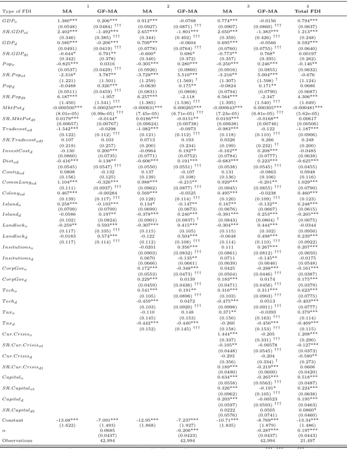
In Table 9, we present our baseline results using the full sample. The table presents four specifications. The first specification includes only measures of market size and international barriers. The second adds controls for the economic and political climate of the origin and destination. The third, which is our preferred specification, further adds variables relating to currency crises and capital market depth. In each of these, the first column presents the coefficients for our non-interacted controls. The second column presents the coefficients for the controls interacted with GFmodt, i.e. the estimated difference between the effect on MA
and GF with the sum of the two the estimated total effect for GF. The significance of this total effect is indicated by the†s on the standard error of the interacted variable (something particularly of interest when the interacted and non-interacted coefficients differ in sign). The fourth specification uses total number of FDI projects as the dependent variable, i.e. it does not distinguish between modes. This is included in order to compare our estimates with those that would be obtained could we not differentiate between GF and MA.
Looking across the first three specifications, we see that the inclusion of additional vari-25When omitting some controls, as in Specification 1, it is possible to expand the number of countries
included. Doing so yields results very comparable to what we present. Therefore, rather than have different samples across specifications, we restrict our sample accordingly.
ables can affect the estimates (for example, when including the political and economic vari-ables, we no longer find differences between MA and GF responses to long run GDPs). However rather than elaborate on these cross-specification differences, for brevity we focus only on the estimates of the preferred specification.
Beginning with our market size variables, we find that higher origin and destination long-run GDPs increase FDI in both modes with no significant difference between them. Short-run increases in origin GDP also increase FDI in both modes, although the effect is only one-third as large for GF. In contrast, short run increases in destination GDP reduce the number of MA yet have no effect on GF. Thus, although the two modes react similarly to persistent GDP patterns, GF is less responsive to short run variations. Similarly, higher origin population, both in the long and short run, reduce MA activity (which given the log form and the inclusion of GDP, is best interpreted as more MA coming from wealthier countries as per Nocke and Yeaple, 2008). However, there is no significant impact from origin population on GF. On the other hand, long-run destination population encourages only GF. Since MA is in part about acquiring new technologies whereas GF is primarily about locating the firm’s existing technology in the most profitable (i.e. low cost) location, this result may reflect the relative attractiveness of low destination wages for GF (an interpretation that is supported by the fact that GF is generally headed to developing countries). Short run destination population increases are correlated with more FDI of both modes, although as with destination GDP, the effect is muted for GF. Combining these results, the broad picture is that FDI of both modes is attracted to larger markets, mirroring the existing literature. Further, origin income is a driver for MA but not GF. Finally, on the whole, GF appears less sensitive to short run variations than does MA, a result that has not been documented to this point. Destination market potential is negatively correlated with FDI in both modes. Although this negative coefficient is a common finding, it is not consistent with existing models of FDI.27 This effect is twice as large for MA as GF investment. Short run boosts in
market potential, however, significantly increase MA but not GF. Thus, proximity to other markets has somewhat mixed effects. In any case, as the coefficients are quite small, our estimates suggest that the importance of surrounding market potential is swamped by the importance of the destination market’s size.
Turning to our trade barrier measure, we find that long run trade costs are a significant and equal detriment to both modes. Short run variations, however, have no significant effect. In contrast, investment costs reduce MA but have no significant effect on GF. Across our other barrier measures, we find that GF is generally less responsive to barriers. While both modes are deterred by the distance between countries, the effect for GF is a third smaller. This is comparable to the finding of Hebous et al. (2011). Similarly, while a common language boosts both modes, the effect is muted for GF. To the extent that these control for cultural differences, this is in in line with Neto et al. (2009) and Drogendijk and Slangen (2006). A similar finding is found for the island and landlocked variables. Contiguity has no impact on either mode. Thus, we find that on the whole FDI is reduced by differences in location, language, and history, but that these matter more for MA than GF investment. This would be consistent with the notion that to reap the benefits of MA requires integration between the acquiring firm and the target whereas GF does not.
In comparison, only GF responds to institutional quality, tending to come from countries with strong institutions and go to locations with weaker institutions. We hesitate to suggest that this means GF is attracted to weak institutions, however, since it may simply capture that the predominance of GF flows to developing countries. This is one reason for con-sidering direction-specific FDI flows. Stronger corporate governance encouraging inflows of both modes but is negatively correlated with GF outflows (suggesting that better corporate governance in the origin may encourage firms to locate new production facilities there rather than offshore). Higher origin technology levels, increases both modes, particularly GF. This again is consistent with the notion that GF must rely more on what the firm brings with it from the origin country. Higher technology in the destination, on the other hand, reduces
GF and MA equally.
Both modes see higher outbound flows when the origin tax is higher, a result suggestive of investment seeking low-tax locations. In this vein, we find negative coefficients for the destination tax variables, however, this is significant only for GF. This is consistent with Hebous et al. (2011) and Swenson (2001) and the theory of Becker and Fuest (2010).
Turning to the crisis variables, we find that more MA comes from countries with higher average crisis numbers but that there is no effect on GF. This may be due to investors in such countries seeking safer investment opportunities elsewhere, leading them to purchase more foreign assets. Both modes, however, fall when the origin country is actually experiencing a currency crisis. Looking to the destination, the only significant effect is that inbound MA rises during a currency crisis, a result suggestive of the fire sale argument and consistent with the results of Blonigen (1997). Thus, as in Klein and Rosengren (1994), we find that MA is more sensitive to exchange rate changes than is GF. Finally, greater capital market depth in either location encourages more FDI in either mode, although the impact of origin capital market depth on GF is half as large. This then recalls the unilateral estimates of Globerman and Shapiro (2004). In addition, as with the other variables, although both modes increase with a short-run increase in origin capital market depth, the effect is significantly smaller for GF. This is in line with Baker et al. (2009), who find evidence for their “cheap finan-cial hypothesis”, in which FDI flows reflect the opportunistic use of the relatively low-cost financial capital available to overvalued parents in the source country.
Thus, our estimates suggest that GF and MA investments follow broadly similar patterns but that there are noticeable differences. On the whole, GF is less responsive to international barriers, short run market size variations, destination currency devaluations, and origin capital market depth, but is more responsive to destination tax rates and origin technological development.
Finally, turning to the fourth specification which uses total FDI as the dependent variable, we unsurprisingly find a comparable overall pattern with the coefficients lying between those
for MA and the total GF effects.
5.2
North versus South results
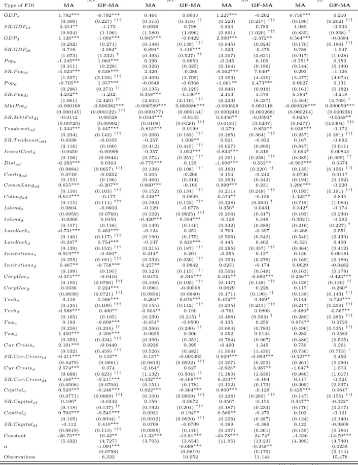
In Table 10, we break the sample into four sub-samples: NN, NS, SN, and SS respectively. Thus the first two specifications relate to investment originating the developing countries and the odd-numbered specifications describe FDI destined for the developed countries.
Beginning with the market size variables, we see that the sign of the coefficients are on the whole comparable to those found in the baseline results. What differs considerably, however, is the significance across sub-samples. The significance of the origin and destination GDP and populations are higher for the NN sub-sample than in the others (despite this being by far the smallest sample). That said, long run GDP, be that for the origin or destination, tends to increase FDI in both modes across all sub-samples. For NN FDI, it is worth recognizing that these effects are significantly smaller for GF than MA FDI. Recall that this is what Globerman and Shapiro (2004) found for their entire sample of unilateral data where they were unable to make country-pair comparisons. Further, the result from the baseline that GF is attracted to a higher long run population (and thus lower average wage) location seems to be a feature of GF FDI destined for the North, regardless of its origin. In contrast, long run destination population in the South has no effect (possibly due to a greater conflict between the attraction of low wages for employees and the repulsion of low wages of potential consumers). For market potential, we find the opposite as it is far more significant for FDI destined to the South than the North, regardless of the origin. Together these suggest that country-pair markets are particularly important for FDI between developing countries whereas proximity to third markets matters more for developing nations.
Long run trade barriers reduce FDI in all cases, although for SN FDI, this is true only for GF. Similarly, distance, common language, and colonial history are roughly comparable across sub-samples in sign, although the magnitude of coefficients differs somewhat. For example, distance has a similar impact in the NS, SN, and SS sub-samples, but a much
smaller coefficient in the NN regression.28 A second noticeable difference compared to the
baseline is that only in the SN sub-sample does GF respond differently than MA (where as in the baseline it is less responsive to distances). Given the various concentrations in modes across these sub-samples, this suggests that some of the differences picked up in Table 9 may have been due to differences between NN FDI and that involving developing countries rather than those between GF and MA. Another key difference across samples is the importance of institutions, which matter only for FDI originating in the developed countries. In particular, note that the puzzling negative coefficient on destination institutions has disappeared. Instead, we find that, as one might expect, better destination institutions attract FDI, a result that is particularly true for MA FDI between developed countries. A common result across sub-samples is that higher levels of origin technological development (be that origin developed or developing) is correlated with more outbound GF but not MA FDI.
The coefficients on the tax variables also differs across the sub-samples. Higher origin taxes are correlated with greater outflows in both modes for FDI between developing coun-tries. In contrast, GF FDI within the developed world is negatively correlated with origin taxes. Destination taxes are now only significant for FDI within the North. Somewhat per-versely, it suggests that MA is actually attracted to higher destination taxes; GF, however, remains negatively correlated with the destination tax.29
FDI from the North is where most of the significance of the currency crisis variables are found. On the whole, they are consistent with the baseline estimates. One difference, however, is in the SN results where during a crisis in the origin country, MA outflows sig-nificantly increase. This is suggestive of the possibility of capital flight during such episodes with investors in the South seeking a safe haven in the North. In a comparable fashion, 28One interpretation of this result would be that NN FDI has a greater concentration of market-seeking
horizontal FDI, a form of investment which is increasing in trade costs, whereas the others have a greater vertical (or factor-seeking) component.
29Note that due to data availability, our dataset does not include the bulk of the tax haven countries (most
our capital market depth variables matter most for NN FDI where the findings again mirror those in the baseline.
Combining these, we see that there are indeed differences in the patterns of FDI depending on the number of developed countries it involves. On the whole, FDI between developed countries (which recall is the largest share of total flows) match the baseline results. Further, allowing the coefficients to vary according to the direction of flows reduces some of the differences between MA and GF. However, we still find that GF is generally less sensitive to short-run market size variation than is MA but that it is much more sensitive to destination tax rates and origin technological development.
5.3
Sector results
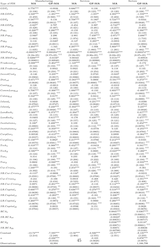
Table 11 utilizes the sector information in our data. Unfortunately, finding data at the sector level across countries and time is difficult and we are therefore limited in our ability to include sector-level controls. Nevertheless, we examine the data in two ways.
First, specifications 1 and 2 repeat the baseline but using only manufacturing and services projects respectively (i.e. the dependent variable in specification 1 is the number of manu-facturing projects in mode m from o to d in t). On the whole, the estimated coefficients are similar across industries and to the baseline estimates. Nevertheless, differences do emerge. For example, while trade costs reduce all modes in both sectors, the impact on MA is half as large in manufacturing as in services; GF meanwhile has a roughly comparable response in both industries. In addition, while distance lowers both modes in both industries, we see a relative unresponsiveness in GF manufacturing but not in GF services. Origin technology, on the other hand increases both modes in both industries with an even stronger effect for outbound manufacturing GF. Institutions are significant for manufacturing but not for ser-vices; a common language however is more important for services than manufacturing. The only significant tax coefficient is found on manufacturing GF, where as before, we find that higher destination taxes mean less investment. Thus, we find that on the whole the two
industries have similar patterns but that certain factors (such as destination population or language barriers) are more important in one industry than in another, with these differences in line with what one might expect for these broad industry categories.
Specification 3 uses data at the country-pair, mode, year, and sector level. Recall that with these data, we augment the baseline specification by including sector dummies (includ-ing their interactions with the GF dummy) and both long run and short run measures of RCA. As can be seen, the coefficients are generally comparable to those in the baseline (al-though with the rise in the number of observations, we see a rise in significance). Focusing on the RCA variables, we see that higher long-run RCA increases both inbound and outbound FDI in both modes, indicating a comparative advantage component to both the creation of outbound FDI and the ability to attract it. In addition, having a stronger comparative advantage tends to increase GF more than it does MA, again suggesting the importance of the development of firm-specific assets at home for GF investment relative to MA. Short run variations in comparative advantage, however, have no effect.
6
Conclusion
FDI is a dominant feature in the global economy, with intra-firm trade accounting for a third of global trade flows (Lanz and Miroudot, 2009). One long-recognized aspect of FDI is that it takes place for a variety of different reasons and through different modes, namely mergers and acquisitions and greenfield investment. Nevertheless, data constraints have hindered a systematic comparison of these two modes of investment. This paper has sought to fill that gap.
Using worldwide data on MA and GF for 2003-2010, we find that in terms of numbers the majority of worldwide flows are GF, although MA likely accounts for approximately 77.5% of the value of those flows. Unsurprisingly, the bulk of investment in both modes comes from the developed countries, with developed countries also the primary destinations for MA. In
contrast, most GF goes to the developing world. With respect to the sectoral composition of FDI, three sectors (Software & IT services, Business Services, and Financial Services) dominate flows in both modes. That said, there are differences in the sectoral composition, particularly when comparing sectors between developed and developing countries. Using regression analysis, we find that the broad pattern of MA and GF investments are similar. In particular, we find that both are attracted to larger markets and flourish when the bar-riers between countries are smaller. Nevertheless, we do find differences between them. It is important to highlight that these results are consistent with the conceptual distinction between the two modes. In case of GF, the investing firm relies on its own capacities which are closely related to home attributes. A MA transaction, on the other hand, involves a transfer of ownership and an integration process and as such may exhibit more opportunis-tic behaviour. These differences may then go hand in hand with the observation that MA are very much a developed country phenomenon whereas developing countries are much more represented in GF activity.
Taken as a whole, these results are reassuring in that they suggest that the current state of understanding of FDI patterns is not overly sensitive to the distinction between FDI modes. Nevertheless, given the differences and in particular certain countries attract certain modes, recognizing the differences between MA and GF is potentially important to reconciling the varying results found across different data sets. Furthermore, our results suggest that policies intending to influence FDI may have a differential impact across modes. For example, cutting one’s tax rates may lead to more inbound GF investment but not additional MA. Similarly, working to upgrade the technological development of a country is more likely to encourage outbound GF investment than MA. To the extent that these have different impacts on an economy (see Davies and Desbordes (forthcoming) for an example), this may be important when developing policy. Thus, although this exercise has been largely descriptive, it makes a significant contribution in terms of our understanding of FDI and of the sometimes contradictory literature that has been written about it.
References
Aguiar, M. and Gopinath, G. (2005). Fire-sale foreign direct investment and liquidity crises. Review of Economics and Statistics, 87(3):439–452.
Armstrong, S. (2009). Japanese fdi in china: determinants and performance. Asia Pacific Economic Papers 378, Australia-Japan Research Centre, Crawford School of Public Policy, The Australian National University.
Azemar, C., Darby, J., Desbordes, R., and Wooton, I. (2012). Market Familiarity and the Location of South and North MNEs. Economics and Politics, 24(3):307–345.
Baker, M., Foley, C. F., and Wurgler, J. (2009). Multinationals as Arbitrageurs: The Effect of Stock Market Valuations on Foreign Direct Investment. Review of Financial Studies, Society for Financial Studies, 22(1):337–369.
Balassa, B. (1964). The Purchasing-Power Parity Doctrine: A Reappraisal. Journal of Political Economy, 72:584.
Beck, T., Demirguc-Kunt, A., and Levine, R. (2009). Financial institutions and markets across countries and over time - data and analysis. Policy Research Working Paper Series No. 4943.
Becker, J. and Fuest, C. (2010). Taxing Foreign Profits with International Mergers and Acquisitions. International Economic Review, 51(1):171–186.
Blonigen, B. (2005). A Review of the Empirical Literature on FDI Determinants. Atlantic Economic Journal, 33(4):383–403.
Blonigen, B. A. (1997). Firm-specific assets and the link between exchange rates and foreign direct investment. American Economic Review, 87(3):447–465.
Blonigen, B. A., Davies, R. B., Waddell, G. R., and Naughton, H. (2007). Fdi in space: Spa-tial autoregressive relationships in foreign direct investment. European Economic Review, 51(5):1303–1325.
Blonigen, B. A., Fontagne, L., Sly, N., and Toubal, F. (2012). Cherries for Sale: Export Networks and the Incidence of Cross-Border M&A. NBER Working Papers 18414, National Bureau of Economic Research, Inc.
Blonigen, B. A. and Piger, J. (2011). Determinants of foreign direct investment. NBER Working Paper, No. 16704.
Buckley, P. and Casson, M. (1998). Analyzing Foreign Market Entry Strategies: Extending the Internalization Approach. Journal of International Business Studies, 29(3):539 – 561. Coeurdacier, N., De Santis, R. A., and Aviat, A. (2009). Cross-border mergers and
Davies, R. B. and Desbordes, R. (forthcoming). Greenfield fdi and skill upgrading: a po-larised issue. Canadian Journal of Economics.
Davies, R. B. and Guillin, A. (forthcoming). How far away is an intangible? services fdi and distance. World Economy.
Desbordes, R. and Wei, S.-J. (2014). The effects of financial development on foreign direct investment. Technical report, World Bank Policy Research Working Paper 7065.
di Giovanni, J. (2005). What drives capital flows? The case of cross-border M&A activity and financial deepening. Journal of International Economics, Elsevier, 65(1):127–149. DiGuardo, M., Marrocu, E., and Paci, R. (2013). The Concurrent Impact of Cultural,
Political, and Spatial Distances on International Mergers and Acquisitions. Working Paper CRENoS 201308, Centre for North South Economic Research, University of Cagliari and Sassari, Sardinia.
Drogendijk, R. and Slangen, A. (2006). Hofstede, Schwartz, or managerial perceptions? The effects of different cultural distance measures on establishment mode choices by multina-tional enterprises. Internamultina-tional Business Review, 15(4):361–380.
Feenstra, R. C., Inklaar, R., and Timmer, M. P. (2013). The next generation of the penn world table.
Foundation, H. (2013). Index of economic freedom.
Francois, J. and Pindyuk, O. (2014). Consolidated Data on International Trade in Services. Working paper.
Froot, K. A. and Stein, J. C. (1991). Exchange Rates and Foreign Direct Investment: An Imperfect Capital Markets Approach. Quarterly Journal of Economics, 106(4):1191–1217. Gaulier, G. and Zignago, S. (2010). BACI: International Trade Database at the
Product-Level. The 1994-2007 Version. Working Papers 2010-23, CEPII research center.
Globerman, S. and Shapiro, D. (2004). Assessing International Mergers And Acquisitions As A Mode Of Foreign Direct Investment. International Finance 0404009, EconWPA. G¨org, H. (2000). Analysing Foreign Market Entry: The Choice between Greenfield
Invest-ment and Acquisitions. Journal of Economic Studies, 27(3):165–181.
Guadalupe, M., Kuzmina, O., and Thomas, C. (2012). Innovation and Foreign Ownership. American Economic Review, 102(7):3594–3627.
Head, K. and Ries, J. (2008). FDI as an outcome of the market for corporate control: Theory and evidence. Journal of International Economics, 74(1):2–20.
Hebous, S., Ruf, M., and Weichenrieder, A. J. (2011). The Effects Of Taxation On The Location Decision Of Multinational Firms: M&A Versus Greenfield Investments. National Tax Journal, 64(3):817–38.
Helpman, E. (1984). A Simple Theory of International Trade with Multinational Corpora-tions. Journal of Political Economy, 92(3):451–71.
Helpman, E., Melitz, M. J., and Yeaple, S. R. (2004). Export Versus FDI with Heterogeneous Firms. American Economic Review, 94(1):300–316.
Herger, N. and McCorriston, S. (2014). Horizontal, Vertical, and Conglomerate FDI: Evi-dence from Cross Border Acquisitions. Working Papers 14.02, Swiss National Bank, Study Center Gerzensee.
Hur, J., Parinduri, R. A., and Riyanto, Y. E. (2011). Cross-border m&a inflows and quality of country governance: Developing versus developed countries,. Pacific Economic Review, 16(5):638–655.
Hyun, H.-J. and Kim, H. H. (2007). The Determinants of Cross-border M&As : the Role of Institutions and Financial Development in Gravity Model. Finance Working Papers 21934, East Asian Bureau of Economic Research.
Kaufmann, D., Kraay, A., and Mastruzzi, M. (2011). The worldwide governance indicators: methodology and analytical issues. Hague Journal on the Rule of Law, 3(02):220–246. Klein, M. W. and Rosengren, E. S. (1994). The Real Exchange Rate and Foreign Direct
Investment in the United States: Relative Wealth vs. Relative Wage Effects. Journal of International Economics, 36(3-4):373–389.
KPMG (2012). Kpmg international, corporate and indirect tax survey. http: //www.kpmg.com/Global/en/IssuesAndInsights/ArticlesPublications/Documents/ corporate-indirect-tax-survey.pdf.
Krugman, P. (2000). Fire-Sale FDI. In Capital Flows and the Emerging Economies: Theory, Evidence, and Controversies, NBER Chapters, pages 43–58. National Bureau of Economic Research, Inc.
Lanz, R. and Miroudot, R. (2009). Intra-Firm Trade. Patterns, Determinants and Policy Implications. OECD Publishing, 114.
Loretz, S. (2008). Corporate taxation in the OECD in a wider context. Oxford Review of Economic Policy, 24(4):639–660.
Markusen, J. R. (1984). Multinationals, multi-plant economies, and the gains from trade. Journal of International Economics, 16(3-4):205–226.
Mayer, T. and Zignago, S. (2006). Notes on cepii’s distances measures. MPRA Paper 26469, University Library of Munich, Germany.
Muller, T. (2007). Analyzing Modes of Foreign Entry: Greenfield Investment versus Acqui-sition. Review of International Economics, 15(1):93–111.
Navaretti, G. and Venables, A. (2006). Multinational Firms in the World Economy. Princeton University Press.
Neary, J. P. (2007). Cross-Border Mergers as Instruments of Comparative Advantage. Review of Economic Studies, 74(4):1229–1257.
Neto, P., Brando, A., and Cerqueira, A. (2009). The Macroeconomic Determinants of Cross Border Mergers and Acquisitions and Greenfield Investments. GEE Papers 0017, Gabinete de Estratgia e Estudos, Ministrio da Economia e da Inovao.
Nocke, V. and Yeaple, S. (2007). Cross-border mergers and acquisitions vs. greenfield foreign direct investment: The role of firm heterogeneity. Journal of International Economics, 72(2):336–365.
Nocke, V. and Yeaple, S. (2008). An Assignment Theory of Foreign Direct Investment. Review of Economic Studies, 75(2):529–557.
Novi, D. (2013). Gravity Redux: Measuring International Trade Costs with Panel Data. Economic Inquiry, 51(1):101–121.
Park, C.-Y., Byun, H.-S., and Lee, H.-H. (2012). Assessing Factors Affecting M&As versus Greenfield FDI in Emerging Countries. Papers and Briefs, Economics Working Papers 18414, National Bureau of Economic Research, Inc.
Rabe-Hesketh, S. and Skrondal, A. (2012). Multilevel and Longitudinal Modeling Using Stata, Volume I. Stata Press, third edition.
Raff, H., Ryan, M., and Sthler, F. (2009). The choice of market entry mode: Greenfield in-vestment, M&A and joint venture. International Review of Economics & Finance, 18(1):3– 10.
Ray, A. (2014). Expanding Multinationals - Industry Relatedness and Conglomerate M&A. Working paper, Paris School of Economics, Mimeo.
Reinhart, C. M. and Rogoff, K. S. (2010). From financial crash to debt crisis. NBER Working Paper, No. 15795.
Rossi, S. and Volpin, P. F. (2004). Cross-country determinants of mergers and acquisitions. Journal of Financial Economics, 74(2):277–304.
Slangen, A. and Hennar, J.-F. (2007). Greenfield or acquisition entry: A review of the empirical foreign establishment mode literature. Journal of International Management, 13(4):403–429.
Swenson, D. L. (2001). Transaction type and the effect of taxes on the distribution of foreign direct investment in the united states. In Hines, J. J., editor, International Taxation and Multinational Activity, pages 89–112. University of Chicago Press.
UNCTAD (2014). World Investment Report 2014. United Nations, New York and Geneva. Wikipedia (2014a). List of island countries countries.
World Bank (2013). World development indicators.