Patterns of deformations of P 3 and P 4 breathers solutions to the NLS equation

HAL Id: hal-01276394

https://hal.archives-ouvertes.fr/hal-01276394

Preprint submitted on 19 Feb 2016

HAL is a multi-disciplinary open access

archive for the deposit and dissemination of

sci-entific research documents, whether they are

pub-lished or not. The documents may come from

teaching and research institutions in France or

L’archive ouverte pluridisciplinaire HAL, est

destinée au dépôt et à la diffusion de documents

scientifiques de niveau recherche, publiés ou non,

émanant des établissements d’enseignement et de

recherche français ou étrangers, des laboratoires

Patterns of deformations of P 3 and P 4 breathers

solutions to the NLS equation

Pierre Gaillard, Mickaël Gastineau

To cite this version:

Pierre Gaillard, Mickaël Gastineau. Patterns of deformations of P 3 and P 4 breathers solutions to

the NLS equation. 2016. �hal-01276394�

Patterns of deformations of P

3

and P

4

breathers solutions to the NLS

equation.

+

_{Pierre Gaillard,}

Micka¨

el Gastineau

+

_Universit´

_{e de Bourgogne,}

9 Av. Alain Savary, Dijon, France : Dijon, France :

e-mail: Pierre.Gaillard@u-bourgogne.fr,

×

IMCCE, Observatoire de Paris, PSL Research University,

CNRS, Sorbonne Universit´

e, UPMC Univ Paris 06, Univ. Lille,

77 Av. Denfert-Rochereau, 75014 Paris, France :

e-mail: gastineau@imcce.fr

February 19, 2016

Abstract

In this article, one gives a classification of the solutions to the one di-mensional nonlinear focusing Schr¨odinger equation (NLS) by considering the modulus of the solutions in the (x, t) plan in the cases of orders 3 and 4. For this, we use a representation of solutions to NLS equation as a quotient of two determinants by an exponential depending on t. This formulation gives in the case of the order 3 and 4, solutions with respec-tively 4 and 6 parameters. With this method, beside Peregrine breathers, we construct all characteristic patterns for the modulus of solutions, like triangular configurations, ring and others.

1

Introduction

The rogue waves phenomenon currently exceed the strict framework of the study of ocean’s waves [1, 2, 3, 4] and play a significant role in other fields; in non-linear optics [5, 6], Bose-Einstein con-densate [7], superfluid helium [8], at-mosphere [9], plasmas [10], capillary phenomena [11] and even finance [12]. In the following, we consider the one dimensional focusing nonlinear equa-tion of Schr¨odinger (NLS) to describe the phenomena of rogue waves. The first results concerning the NLS equa-tion date from the Seventies. Precisely, in 1972 Zakharov and Shabat solved it using the inverse scattering method [13, 14]. The case of periodic and al-most periodic algebro-geometric solu-tions to the focusing NLS equation were first constructed in 1976 by Its and Kotl-yarov [15, 16]. The first quasi rational solutions of NLS equation were con-structed in 1983 by Peregrine [17]. In 1986 Akhmediev, Eleonskii and Kula-gin obtained the two-phase almost pe-riodic solution to the NLS equation and obtained the first higher order analogue of the Peregrine breather[18, 19, 20]. Other analogues of the Peregrine brea-thers of order 3 and 4 were constructed in a series of articles by Akhmediev et al. [21, 22, 23] using Darboux trans-formations.

The present paper presents multi-para-metric families of quasi rational solu-tions of NLS of order N in terms of de-terminants of order 2N dependent on 2N − 2 real parameters.

The aim of this paper is to try to dis-tinguish among all the possible confi-gurations obtained by different choices of parameters, one those which have a characteristic in order to try to give a classification of these solutions.

2

Expression of

solu-tions of NLS

equa-tion in terms of a

ra-tio of two

determi-nants

We consider the focusing NLS equation ivt+ vxx+ 2|v|2v = 0. (1)

To solve this equation, we need to con-struct two types of functions fj,k and

gj,kdepending on many parameters.

Be-cause of the length of their expressions, one defines the functions fν,µand gν,µ

of argument Aν and Bν only in the

ap-pendix.

We have already constructed solutions of equation NLS in terms of determi-nants of order 2N which we call solu-tion of order N depending on 2N − 2 real parameters. It is given in the fol-lowing result [24, 25, 26, 27] :

Theorem 2.1 The functions v defined by

v(x, t) = det((njk)j,k∈[1,2N ]) det((djk)j,k∈[1,2N ])

e2it−iϕ ₍₂₎

are quasi-rational solution of the NLS equation (1) depending on 2N − 2 pa-rameters ˜aj, ˜bj, 1 ≤ j ≤ N − 1, where nj1= fj,1(x, t, 0), njk= ∂ 2k−2_f j,1 ∂ǫ2k−2 (x, t, 0), njN+1= fj,N+1(x, t, 0), njN+k= ∂ 2k−2_f j,N +1 ∂ǫ2k−2 (x, t, 0), dj1= gj,1(x, t, 0), djk= ∂ 2k−2_g j,1 ∂ǫ2k−2 (x, t, 0), djN+1= gj,N+1(x, t, 0), djN+k=∂ 2k−2_g j,N +1 ∂ǫ2k−2 (x, t, 0), 2 ≤ k ≤ N, 1 ≤ j ≤ 2N (3)

The functions f and g are defined in (9),(10), (11), (12).

3

Patterns of quasi

ra-tional solutions to the

NLS equation

The solutions vN to NLS equation (2)

of order N depending on 2N − 2 pa-rameters ˜aj, ˜bj (for 1 ≤ j ≤ N − 1)

has been already explicitly constructed and can be written as

vN(x, t) = n(x, t) d(x, t)exp(2it) = (1−αN GN(2x, 4t) + iHN(2x, 4t) QN(2x, 4t) )e2it with GN(X, T ) =P N(N +1) k=0 gk(T )Xk, HN(X, T ) =PN (N +1 k=0 hk(T )Xk, QN(X, T ) =P N(N +1 k=0 qk(T )Xk.

For order 3 these expressions can be found in [28]; in the case of order 4, they can be found in [29]. In the fol-lowing, based on these analytic expres-sions, we give a classification of these solutions by means of patterns of their modulus in the plane (x; t).

3.1

Patterns of quasi

ratio-nal solutions of order

3

with

4 parameters

3.1.1 P3 breather

If we choose all parameters equal to 0, ˜

a1= ˜b1 = . . . = ˜aN −1= ˜bN −1= 0, we

obtain the classical Peregrine breather given by

Figure 1: Solution P3 to NLS, N=3,

˜

a1= ˜b1= ˜a2= ˜b2= 0.

3.1.2 Triangles

To shorten, the following notations are used : for example the sequence 1A3 + 1T 3 means that the structure has one arc of 3 peaks and one triangle of 3 peaks.

If we choose ˜a1 or ˜b1 not equal to 0

and all other parameters equal to 0, we obtain triangular configuration with 6 peaks.

Figure 2: Solution 1T 6 to NLS, N=3, ˜

Figure 3: Solution 1T 6 to NLS, N=3, ˜

a1= 0, ˜b1= 104, ˜a2= 0, ˜b2= 0.

3.1.3 Rings

If we choose ˜a2or ˜b2not equal to 0, all

other parameters equal to 0, we obtain ring configuration with peaks.

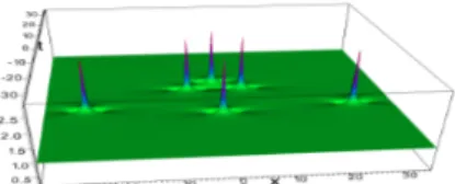
Figure 4: Solution 1R5 + 1 to NLS, N=3, ˜a1= 0, ˜b1= 0, ˜a2= 106, ˜b2= 0.

Figure 5: Solution 1R5 + 1 to NLS, N=3, ˜a1= 0, ˜b1= 0, ˜a2= 0, ˜b2= 105.

3.1.4 Arcs

If we choose ˜a1 and ˜a2 not equal to

0 and all other parameters equal to 0

(and vice versa, ˜b1 and ˜b2not equal to

0 and all other parameters equal to 0), we obtain deformed triangular config-uration which can call arc structure.

Figure 6: Solution 1A3 + 1T 3 to NLS, N=3, ˜a1 = 0, ˜b1 = 104, ˜a2 = 0, ˜b2 =

5 × 106_.

Figure 7: Solution 1A3 + 1T 3 to NLS, N=3, ˜a1 = 106, ˜b1 = 0, ˜a2 = 1010,

˜b2= 0.

3.2

Patterns of quasi

ratio-nal solutions of order

4

with

6 parameters

3.2.1 P4 breather

If we choose all parameters equal to 0, ˜

a1= ˜b1= . . . = ˜aN −1= ˜bN −1= 0, we

obtain the classical Peregrine breather given in the following figure

Figure 8: Solution P4 to NLS, N=4,

˜

a1= ˜b1= ˜a2= ˜b2= ˜a3= ˜b3= 0.

3.2.2 Triangles

To shorten, we use the notations de-fined in the previous section.

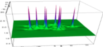
If we choose ˜a1 or ˜b1 not equal to 0

and all other parameters equal to 0, we obtain triangular configuration with 10 peaks. Figure 9: Solution 1T 10 to NLS, N=4, ˜ a1 = 103, ˜b1 = 0, ˜a2 = 0, ˜b2 = 0, ˜ a3= 0, ˜b3= 0. 3.2.3 Rings

If we choose ˜a2 or ˜a3 not equal to 0

and all other parameters equal to 0 (or vice versa ˜b2 or ˜b3 not equal to 0 and

all other parameters equal to 0), we ob-tain ring configuration with 10 peaks.

Figure 10: Solution 2R5/5 to NLS, N=4, ˜a1= 0, ˜b1= 0, ˜a2= 105, ˜b2= 0, ˜ a3= 0, ˜b3= 0. Figure 11: Solution 1R7 + P2 to NLS, N=4, ˜a1 = 0, ˜b1 = 0, ˜a2 = 0, ˜b2 = 0, ˜ a3= 108, ˜b3= 0. 3.2.4 Arcs

If we choose two parameters non equal to 0, ˜a1and ˜a2, or ˜a1and ˜a3 not equal

to 0, or ˜a2 and ˜a3 and all other

pa-rameters equal to 0 (or vice versa for parameters b), we obtain arc configu-ration with 10 peaks1_.

Figure 12: Solution 2A3/4I + T 3 to NLS, N=4, ˜a1= 103, ˜b1= 0, ˜a2= 106,

˜b2= 0, ˜a3= 0, ˜b3= 0.

1_{In the following notations 2A4/3I, I}

Figure 13: Solution 2A3/4I + T 3 to NLS, N=4, ˜a1= 103, ˜b1= 0, ˜a2= 106,

˜b2= 0, ˜a3= 0, ˜b3= 0, sight top.

Figure 14: Solution 2A4/3 + 1T 3 to NLS, N=4, ˜a1 = 103, ˜b1 = 0, ˜a2 = 0,

˜b2= 0, ˜a3= 5 × 107, ˜b3= 0.

Figure 15: Solution 2A4/3 + 1T 3 to NLS, N=4, ˜a1 = 103, ˜b1 = 0, ˜a2 = 0,

˜b2= 0, ˜a3= 5 × 107, ˜b3= 0, sight top.

Figure 16: Solution 2A3/4 + 1T 3 to NLS, N=4, ˜a1 = 0, ˜b1 = 0, ˜a2 = 106,

˜b2= 0, ˜a3= 3 × 108, ˜b3= 0.

Figure 17: Solution 2A3/4 + 1T 3 to NLS, N=4, ˜a1 = 0, ˜b1 = 0, ˜a2 = 106,

˜b2= 0, ˜a3= 3 × 108, ˜b3= 0, sight top.

3.2.5 Triangles inside rings If we choose three parameters non equal to 0, ˜a1, ˜a2and ˜a3and all other

param-eters equal to 0 (or vice versa for pa-rameters b), we obtain ring with inside triangle.

Figure 18: Solution 1A7+1T 3 to NLS, N=4, ˜a1= 103, ˜b1= 0, ˜a2= 103, ˜b2=

Figure 19: Solution 1A7+1T 3 to NLS, N=4, ˜a1= 103, ˜b1= 0, ˜a2= 103, ˜b2=

0, ˜a3= 109, ˜b3= 0, sight top.

4

Conclusion

We recall one more time that the solu-tions at order 3 and 4 to the equation NLS dependent on 4 and 6 parameters were given for the first time by V.B. Matveev [49]. The solutions and their deformations presented here by the au-thors were built later by a completely different method [28], [29].

We have presented here patterns of mo-dulus of solutions to the NLS focusing equation in the (x, t) plane.

These study can be useful at the same time for hydrodynamics as well for non-linear optics; many applications in these fields have been realized, as it can be seen in recent works of Chabchoub et al. [50] or Kibler et al. [51].

This study try to bring all possible types of patterns of quasi rational solutions to the NLS equation.

We see that we can obtain 2N −1

diffe-rent structures at the order N . Parameters a or b give the same type of structure. For a16= 0 (and other

pa-rameters equal to 0), we obtain trian-gular rogue wave; for aj6= 0 (j 6= 1 and

other parameters equal to 0) we get ring rogue wave; in the other choices of parameters, we get in particular arc structures (or claw structure).

This type of study have been realized

in preceding works. Akhmediev et al study the order N = 2 in [52], N = 3 in [53]; the case N = 4 was studied in particular (N = 5, 6 were also stud-ied) in [54, 55] showing triangle and arc patterns; only one type of ring was presented. The extrapolation was done until the order N = 9 in [56]. Ohta and Yang [57] presented the study of the case cas N = 3 with rings and tri-angles. Recently, Ling and Zhao [58] presented the cases N = 2, 3, 4 with rings, triangle and also claw structures. In the present study, one sees appear-ing richer structures, in particular the appearance of a triangle of 3 peaks in-side a ring of 7 peaks in the case of order N = 4; to the best of my knowl-edge, it is the first time that this con-figuration for order 4 is presented. In this way, we try to bring a better understanding to the hierarchy of NLS rogue wave solutions.

It will be relevant to go on this study with higher orders.

References

[1] Ch. Kharif, E. Pelinovsky, A. Slunyaev, Rogue Waves in the Ocean, Springer, (2009).

[2] N. Akhmediev, E. Pelinovsky, Discussion and Debate: Rogue Waves - Towards a unifying con-cept?, Eur. Phys. Jour. Special Topics, V. 185, (2010).

[3] Ch. Kharif, E. Pelinovsky, Physi-cal mechanisms of the rogue wave phenomenon, Eur. Jour. Me-chanics / B - Fluid, V. 22, N. 6, 603-634, (2003).

[4] A. Slunyaev, I. Didenkulova, E. Pelinovsky, Rogue waters, Cont. Phys., V. 52, N. 6, 571-590, (2003).

[5] D.R. Solli, C. Ropers, P. Koonath, B. Jalali, Nature, V. 450, 1054-1057, (2007).

[6] J.M. Dudley, G. Genty,

B.J. Eggleton, Opt. Express, V. 16, 3644, (2008).

[7] Y.V. Bludov, V.V. Konotop, N. Akhmediev, Phys. Rev. A, V. 80, 033610, 1-5, (2009).

[8] A.N. Ganshin, V.B. Efimov, G.V. Kolmakov, L.P. Mezhov-Deglin and P.V.E. McClintok, Phys. Rev. Lett., V. 101, 065303, (2008).

[9] L. Stenflo, M. Marklund, Jour. Of Plasma Phys., , V. 76,N. 3-4, 293-295, (2010).

[10] L. Stenflo, M. Marklund, Eur. Phys. J. Spec. Top., , V. 185, 25002, (2011).

[11] M. Shats, H. Punzman,, H. Xia, Phys. Rev. Lett., V. 104, 104503, 1-5, (2010).

[12] Z.Y Yan, Commun. Theor. Phys., V. 54, N. 5, 947, 1-4, (2010). [13] V.E. Zakharov, J. Appl. Tech.

Phys, V. 9, 86-94, (1968)

[14] V.E. Zakharov, A.B. Shabat Sov.

Phys. JETP, V. 34, 62-69,

(1972)

[15] A.R. Its, V.P. Kotlyarov, Dockl. Akad. Nauk. SSSR, S. A, V. 965., N. 11, (1976).

[16] A.R. Its, A.V. Rybin, M.A. Salle, Teore. i Mat. Fiz., V. 74., N. 1, 29-45, (1988).

[17] D. Peregrine, J. Austral. Math. Soc. Ser. B, V. 25, 16-43, (1983). [18] N. Akhmediev, V. Eleonsky, N. Kulagin, Sov. Phys. J.E.T.P., V. 62, 894-899, (1985).

[19] V. Eleonskii, I. Krichever, N. Ku-lagin, Soviet Doklady 1986 sect. Math. Phys., V. 287, 606-610, (1986).

[20] N. Akhmediev, V. Eleonskii, N. Kulagin, Th. Math. Phys., V. 72, N. 2, 183-196, (1987). [21] N. Akhmediev, A. Ankiewicz,

J.M. Soto-Crespo, Physical Re-view E, V. 80, 026601, 1-9, (2009).

[22] N. Akhmediev, A. Ankiewicz, P.A. Clarkson, J. Phys. A : Math. Theor., V. 43, 122002, 1-9, (2010). [23] A. Chabchoub, H. Hoffmann, M. Onorato, N. Akhmediev, Phys. Review X, V. 2, 011015, 1-6, (2012).

[24] P. Gaillard, J. Phys. A : Meth. Theor., V. 44, 1-15, (2011) [25] P. Gaillard, J. Math. Sciences :

Adv. Appl., V. 13, N. 2, 71-153, (2012)

[26] P. Gaillard, J. Math. Phys., V. 54, 013504-1-32, (2013)

[27] P. Gaillard, Adv. Res., V. 4, 346-364, (2015)

[28] P. Gaillard, Phys. Rev. E, V. 88, 042903-1-9, (2013)

[29] P. Gaillard, J. Math. Phys., V. 54, 073519-1-22, (2013)

[30] P. Gaillard, V.B. Matveev, Max-Planck-Institut f¨ur Mathematik, MPI 02-31, V. 161, (2002) [31] P. Gaillard, Lett. Math. Phys., V.

68, 77-90, (2004)

[32] P. Gaillard, V.B. Matveev, Lett. Math. Phys., V. 89, 1-12, (2009) [33] P. Gaillard, V.B. Matveev, J. Phys A : Math. Theor., V. 42, 1-16, (2009)

[34] P. Gaillard, J. Mod. Phys., V. 4, N. 4, 246-266, (2013) [35] P. Gaillard, V.B. Matveev, J. Math., V. 2013, ID 645752, 1-10, (2013) [36] P. Gaillard, J. Math., V. 2013, 1-111, (2013)

[37] P. Gaillard, J. Theor. Appl. Phys., V. 7, N. 45, 1-6, (2013) [38] P. Gaillard, Phys. Scripta, V. 89,

015004-1-7, (2014)

[39] P. Gaillard, Commun. Theor. Phys., V. 61, 365-369,(2014) [40] P. Gaillard, J. Of Phys. : Conf.

Ser., V. 482, 012016-1-7, (2014) [41] P. Gaillard, M. Gastineau, Int. J. Mod. Phys. C, V. 26, N. 2, 1550016-1-14, (2014)

[42] P. Gaillard, J. Math. Phys., V. 5, 093506-1-12, (2014)

[43] P. Gaillard, J. Phys. : Conf. Ser., V. 574, 012031-1-5, (2015) [44] P. Gaillard, Ann. Phys., V. 355,

293-298, (2015)

[45] P. Gaillard, M. Gastineau, Phys. Lett. A, V. 379, 1309-1313, (2015)

[46] P. Gaillard, J. Phys. A:

Math. Theor., V. 48, 145203-1-23, (2015)

[47] P. Gaillard, Jour. Phys. : Conf. Ser., V. 633, 012106-1-6, 2015 [48] P. Gaillard, M. Gastineau

Com-mun. Theor. Phys, V. 65, 136-144, 2016

[49] P. Dubard, V.B. Matveev, Non-linearity, V. 26,93-125, 2013 [50] A. Chabchoub, N.P. Hoffmann,

N. Akhmediev, Phys. Rev. Lett., V. 106, 204502-1-4, (2011) [51] B. Kibler, J. Fatome, C. Finot,

G. Millot, F. Dias, G. Genty, N. Akhmediev, J.M. Dudley, Na-ture Physics, V. 6, 790-795, (2010)

[52] A. Ankiewicz, D. J. Kedziora, N. Akhmediev, Phys Let. A, V. 375, 2782-2785, (2011)

[53] D. J. Kedziora, A. Ankiewicz, N. Akhmediev, J. Opt., V. 15, 064011-1-9, (2013)

[54] D. J. Kedziora, A. Ankiewicz, N. Akhmediev, Phys. Review E, V. 84, 056611, 1-7, (2011) [55] D.J. Kedziora, A. Ankiewicz,

N. Akhmediev, Phys. Rev. E, V. 86, 056602, 1-9, (2012).

[56] D. J. Kedziora, A. Ankiewicz, N. Akhmediev, Phys. Review E, V. 88, 013207-1-12, (2013) [57] Y Ohta, J. Yang, Proc. Of The

Roy. Soc. A, V. 468, N. 2142, 1716-1740, (2012).

[58] L. Ling, L.C. Zhao, Phys. Rev. E, V; 88, 043201-1-9, (2013) Appendix

Parameters and functions

We consider the terms λνsatisfying the

relations for 1 ≤ j ≤ N 0 < λj< 1, λN+j = −λj,

λj = 1 − 2ǫ2j2,

with ǫ a small number intended to tend towards 0.

The terms κν, δν, γν are functions of

the parameters λν, 1 ≤ ν ≤ 2N . They

are given by the following equations, for 1 ≤ j ≤ N : κj= 2 q 1 − λ2 j, δj= κjλj, γj= q_1−λ j 1+λj, (4) κN+j= κj, δN+j = −δj, γN+j = 1/γj. (5)

The terms xr,ν r = 3, 1 are defined by

xr,j= (r − 1) lnγj −i γj+i,

xr,N+j = (r − 1) lnγ_γN +j_{N +j}−i+i.

(6) The parameters eν are given by

ej = iaj− bj, eN+j= iaj+ bj, (7)

where aj and bjare chosen in the form

aj=PN −1k=1 a˜kǫ2k+1j2k+1,

bj =PN −1k=1 b˜kǫ2k+1j2k+1,

1 ≤ j ≤ N,

(8)

with ˜aj, ˜bj,, 1 ≤ j ≤ N − 1, 2N − 2,

arbitrary real numbers.

The functions fν,1and gν,1, 1 ≤ ν ≤ N

are defined by (here k = 1) : f4j+1,1= γ_k4j−1sin A1, f4j+2,1= γk4jcos A1, f4j+3,1= −γ_k4j+1sin A1, f4j+4,1= −γk4j+2cos A1, (9) f4j+1,N +1= γ_k2N −4j−2cos AN+1, f4j+2,N +1= −γ2N −4j−3k sin AN+1, f4j+3,N +1= −γ2N −4j−4_k cos AN+1, f4j+4,N +1= γ_k2N −4j−5sin AN+1, (10) g4j+1,1= γ_k4j−1sin B1, g4j+2,1= γ_k4jcos B1, g4j+3,1= −γk4j+1sin B1, g4j+4,1= −γ_k4j+2cos B1, (11) g4j+1,N +1= γ_k2N −4j−2cos BN+1, g4j+2,N +1= −γ_k2N −4j−3sin BN+1, g4j+3,N +1= −γk2N −4j−4cos BN+1, g4j+4,N +1= γk2N −4j−5sin BN+1. (12)

The arguments Aνand Bνof these

func-tions are defined by 1 ≤ ν ≤ 2N : Aν= κνx/2 + iδνt − ix3,ν/2 − ieν/2,