Machine learning: Supervised methods, SVM and kNN

HAL Id: hal-01657491

https://hal.archives-ouvertes.fr/hal-01657491

Submitted on 6 Dec 2017

HAL is a multi-disciplinary open access archive for the deposit and dissemination of sci-entific research documents, whether they are pub-lished or not. The documents may come from teaching and research institutions in France or abroad, or from public or private research centers.

L’archive ouverte pluridisciplinaire HAL, est destinée au dépôt et à la diffusion de documents scientifiques de niveau recherche, publiés ou non, émanant des établissements d’enseignement et de recherche français ou étrangers, des laboratoires publics ou privés.

Machine learning: Supervised methods, SVM and kNN

To cite this version:

Danilo Bzdok, Martin Krzywinski, Naomi Altman. Machine learning: Supervised methods, SVM and kNN. Nature Methods, Nature Publishing Group, 2018, pp.1-6. �hal-01657491�

POINTS OF SIGNIFICANCE

Machine learning: Supervised methods, SVM and kNN

Supervised learning algorithms extract general principles from observed examples guided by a specific prediction objective.

In supervised learning, a set of input variables, such as blood metabolite or gene expression levels, are used to predict a

quantitative response variable like hormone level or a qualitative one such as healthy versus diseased individuals. We have previously discussed several supervised learning algorithms, including logistic regression and random forests, and their typical behaviors with different sample sizes and numbers of predictor variables. This month, we look at two very common supervised methods in the context of machine learning: linear support vector machines (SVM) and k-nearest neighbors (kNN). Both have been successfully applied to challenging pattern-recognition problems in biology and medicine [1].

SVM and kNN exemplify several important trade-offs in machine learning (ML). SVM is less computationally demanding than kNN and is easier to interpret but can identify only a limited set of patterns. On the other hand, kNN can find very complex patterns but its output is more challenging to interpret. To illustrate both algorithms, we will apply them to classification because they tend to perform better at predicting categorical outputs (e.g., health versus disease) than at approximating target functions with numeric outputs (e.g., hormone level). Both learning techniques can be used to distinguish many classes at once, use multiple predictors and obtain probabilities for each class membership.

We’ll illustrate SVM using a two-class problem and begin with a case in which the classes are linearly separable, meaning that a straight line can be drawn that perfectly separates the classes with the margin being the perpendicular distance between the closest points to the line from each class (Fig. 1a). Many such separating lines are possible and SVM can be used to find one with the widest margin (Fig. 1b). When three or more predictors are used, the separating line becomes a hyperplane, but the algorithm remains the same. The closest points to the line are called support vectors [1] and are the only points that ultimately influence the position of the separating

line—any points that are further from the line can be moved, removed or added with no impact on the line. When the classes are linearly separable, the wider the margin, the higher our confidence in the classification because it indicates that the classes are less similar.

Figure 1 | A support vector machine (SVM) classifies points by maximizing the width of a margin that separates the classes. (a) Points from two classes (grey, blue) that are perfectly separable by various lines (black) illustrate the concept of a margin (light yellow highlight), which is the rectangular region that extends from the

separating line to the perpendicularly closest point. (b) An SVM finds the line (black) that has the largest margin (0.48). Points at the margin’s edge (black outlines) are called support vectors—the margin is not influenced by moving or adding other points outside it. (c) Imposing a separating line on linearly non-separable classes will incur margin violations and misclassification errors. Data same as in (b) but with two additional points added (those that are misclassified). The margin is now 0.64 with 6 support vectors.

Practically, most data sets are not linearly separable and any

separating line will result in misclassification, no matter how narrow the margin is. We say that the margin is violated by a sample if it is on the wrong side of the separating line (Fig 1c, red arrows) or is on the correct side, but is within the margin (Fig. 1c, orange arrow).

Even when the data are linearly separable, allowing a few points to be misclassified might improve the classifier by allowing a wider margin for the bulk of the data (Fig. 2a). To handle violations, we impose a penalty proportional to the distance between each violating point [1] and the separating line, with non-violating points having zero

penalty. In SVM, the separating line is chosen by minimizing 1/m+C

∑pi where m is the margin width, pi is the penalty for each point and C is a hyper-parameter (a parameter used to tune the overall fitting

width and misclassification. A point that has a non-zero penalty is considered a support vector because it impacts the position of the separating line and its margin.

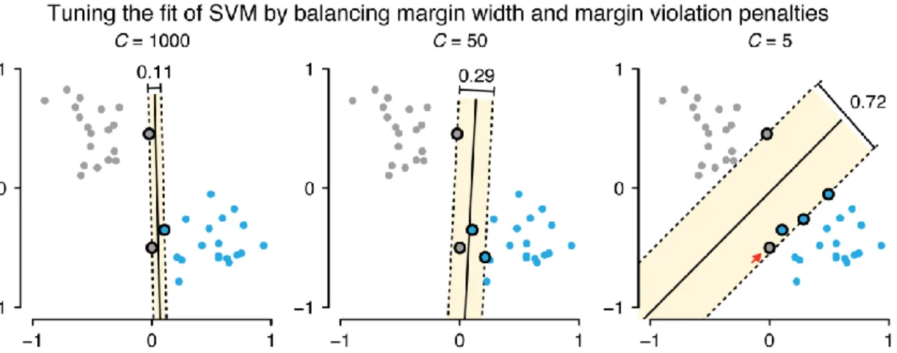
When C is large, the margin width has a low impact on the minimization and the line is placed to minimize the sum of the violation penalties (Fig. 2, C = 1000). When C is decreased, the misclassified points have lower impact and the line is placed with more emphasis on maximizing the margin. (Fig. 2, C = 50 and C = 5). When C is very small, classification penalties become insignificant and the margin can be encouraged to actually grow to encompass all points. Typically, C is chosen using cross-validation [2].

Recall we showed previously [3] how regularization can be used to guard against overfitting which occurs when the prediction equation is too closely tailored to random variation in the training set. In that sense, the role of C is similar, except here it tunes the fit by adjusting the balance of terms being minimized rather than the complexity of the shape of the boundary. Large values of C force the separating line to adjust to data far from the center of each class and thus encourage overfitting. Small values tolerate many margin violations and

encourage underfitting.

Figure 2 | The balance between the width of the margin and penalties for margin violations is controlled by a regularization parameter, C. Smaller values of C places more weight on margin width and less on classification constraints.

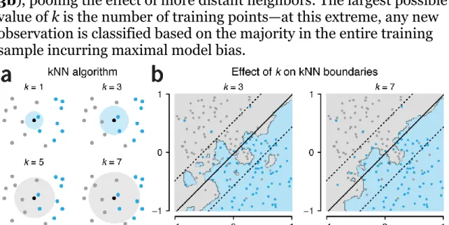
We can avoid the explicit assumption of a linear class boundary by using the k-nearest neighbours (kNN) algorithm. This algorithm determines the class of an unclassified point by counting the majority class vote from its k-nearest neighbour training points (Fig. 3a). For example, a patient whose symptoms closely match those of patients

with a specific diagnosis would be classified with the same disease status. Because kNN does not assume a particular boundary between the classes, its boundary can be closer to the “true” relationship. However, for a given training set, predictions may be less stable than for SVMs, especially when k is small, and the algorithm will often overfit the training data.

The value of k acts to regularize kNN, analogous to C in SVM and is generally selected by cross-validation. To avoid ties in the vote, k can be chosen to be odd. Small k gives a finely-textured boundary which is sensitive to outliers and yields a high model variance (k = 3, Fig. 3b). Larger k gives more rigid boundaries and high model bias (k = 7, Fig. 3b), pooling the effect of more distant neighbors. The largest possible value of k is the number of training points—at this extreme, any new observation is classified based on the majority in the entire training sample incurring maximal model bias.

Figure 3 | Illustration of the k-nearest neighbours (kNN) classifier. (a) kNN assigns a class to an unclassified point (black) based on a majority vote of the k nearest neighbours in the training set (grey and blue points). Shown are cases for k = 1, 3, 5 and 7; the k neighbours are circumscribed in the circle, which is colored by the majority class vote. (b) For k = 3, the kNN boundaries are relatively rough

(calculated by classifying each point in the plane) and give 10% misclassifications. The SVM separating line (black) and margin (dashed) is also shown for C = 1000 yielding 15% misclassification. As k is increased (here, k = 7, 13% misclassifications), single misclassifications have less impact on the emerging boundary, which becomes smoother.

Neither SVM nor kNN make explicit model specifications about the the data-generating process such as normality of the data. However, linear SVM is considered a parametric method because it can only produce linear boundaries. If the true class boundary is nonlinear, SVM will struggle to find a satisfying fit even with increased size of

the training set. To help the algorithm capture nonlinear boundaries, functions of the input variables, such as polynomials, could be added to the set of predictor variables [1]. This extension of the algorithm is called kernel SVM.

In contrast, kNN is a nonparametric algorithm because it avoids a priori assumptions about the shape of the class boundary and can thus adapt more closely to nonlinear boundaries as the amount of training data increases. kNN has higher variance than linear SVM but it has the advantage of producing classification fits that adapt to any boundary. Even though the true class boundary is unknown in most real-world applications, kNN has been shown to approach the

theoretically optimal classification boundary as the training set

increases to massive data [1]. However, because kNN does not impose any structure on the boundary, it can create class boundaries that may be less interpretable than those of linear SVM. The simplicity of the linear SVM boundary also lends itself more directly to formal tests of statistical significance that give P values for the relevance of

individual variables.

There are also trade-offs in the number of samples and the number of variables that can be handled by these approaches. SVM can achieve good prediction accuracy for new observations despite large numbers of input variables. SVM therefore serves as an off-the-shelf technique that is frequently used in genome-wide analysis and brain imaging, two application domains with often low sample sizes (e.g., hundreds of participants) but very high numbers of inputs (e.g., hundreds of thousands of genes or brain locations).

By contrast, the classification performance of kNN rapidly

deteriorates when searching for patterns using high numbers of input variables [1] when many of the variables may be unrelated to the classification or contribute only small amounts of information.

Because equal attention is given to all variables, the nearest neighbors may be defined by irrelevant variables. This so-called curse of

dimensionality occurs for many algorithms that become more flexible as the number of predictors increases [1].

Finally, computation and memory resources are important practical considerations [4]. SVM only needs a small subset of training points (the support vectors) to define the classification rule, making it often more memory efficient and less computationally demanding when inferring the class of a new observation. In contrast, kNN typically

requires higher computation and memory resources because it needs to use all input variables and training samples for each new

observation to be classified.

COMPETING FINANCIAL INTERESTS

The authors declare no competing financial interests.

Danilo Bzdok, Martin Krzywinski & Naomi Altman [1] Hastie, T., Tibshirani, R., Friedman, J. Springer Series in

Statistics, Heidelberg (2001).

[2] Lever, J., Krzywinski, M. & Altman, N. (2016) Points of

significance: Model Selection and Overfitting. Nature Methods

13:703–704.

[3] Lever, J., Krzywinski, M. & Altman, N. (2016) Points of

significance: Regularization. Nature Methods 13:803–804.

[4] Bzdok, D. & Yeo, B.T.T. (2017) NeuroImage, 155: 549-564.

Danilo Bzdok is an Assistant Professor at the Department of

Psychiatry, RWTH Aachen University, in Germany and a Visiting Professor at INRIA/Neurospin Saclay in France. Martin Krzywinski is a staff scientist at Canada’s Michael Smith Genome Sciences

Centre. Naomi Altman is a Professor of Statistics at The Pennsylvania State University.