HAL Id: hal-02993268
https://hal.archives-ouvertes.fr/hal-02993268
Submitted on 6 Nov 2020
HAL is a multi-disciplinary open access
archive for the deposit and dissemination of
sci-entific research documents, whether they are
pub-lished or not. The documents may come from
teaching and research institutions in France or
abroad, or from public or private research centers.
L’archive ouverte pluridisciplinaire HAL, est
destinée au dépôt et à la diffusion de documents
scientifiques de niveau recherche, publiés ou non,
émanant des établissements d’enseignement et de
recherche français ou étrangers, des laboratoires
publics ou privés.
on Saturn’s largest moon, Titan
Chloé Daudon, Antoine Lucas, Sebastien Rodriguez, Stéphane Jacquemoud,
A. Escalante Lopez, B. Grieger, E. Howington-Kraus, E. Karkoschka, R. L.
Kirk, J. T. Perron, et al.
To cite this version:
Chloé Daudon, Antoine Lucas, Sebastien Rodriguez, Stéphane Jacquemoud, A. Escalante Lopez, et
al.. A new digital terrain model of the Huygens landing site on Saturn’s largest moon, Titan. Earth
and Space Science, American Geophysical Union/Wiley, 2020, �10.1029/2020ea001127�. �hal-02993268�
A new digital terrain model of the Huygens landing
1
site on Saturn’s largest moon, Titan
2
C. Daudon1, A. Lucas1, S. Rodriguez1, S. Jacquemoud1, A. Escalante L´opez2, 3
B. Grieger2, E. Howington-Kraus3, E. Karkoschka4, R. L. Kirk3, J. T. Perron5, 4
J. M. Soderblom5, M. Costa2. 5
1Universit´e de Paris, Institut de physique du globe de Paris, CNRS, F-75005, Paris, France
6
2RHEA System for ESA, European Space Astronomy Centre, Camino Bajo del Castillo s/n, Urb.
7
Villafranca del Castillo, E-28692 Villanueva de la Ca˜nada, Madrid, Spain
8
3Astrogeology Science Center, U.S. Geological Survey, 2255 N. Gemini Dr., Flagstaff AZ 86001, USA
9
4Lunar and Planetary Laboratory, 1629 E University Blvd Tucson AZ 85721-0092, USA
10
5Department of Earth, Atmospheric & Planetary Sciences, Massachusetts Institute of Technology, 77
11
Massachusetts Ave, Cambridge MA 02139, USA
12
Key Points:
13
• We create a new digital terrain model (DTM) of the Huygens landing site that 14
offers the best available resolution of river valleys on Titan.
15
• The complexity of the data set requires a tailor-made reconstruction procedure 16
that is detailed.
17
• The workflow uses re-processed Huygens/DISR images and an automated shape-18
from-motion algorithm to improve an earlier DTM.
19
Corresponding author: C. Daudon, [email protected]
–1–
This article has been accepted for publication and undergone full peer review but has not been
through the copyediting, typesetting, pagination and proofreading process which may lead to
differences between this version and the Version of Record. Please cite this article as doi:
10.1029/2020EA001127
Abstract
20
River valleys have been observed on Titan at all latitudes by the Cassini-Huygens
21
mission. Just like water on Earth, liquid methane carves into the substrate to form a
com-22
plex network of rivers, particularly stunning in the images acquired near the equator by
23
the Huygens probe. To better understand the processes at work that form these
land-24
scapes, one needs an accurate digital terrain model (DTM) of this region. The first and
25
to date the only existing DTM of the Huygens landing site was produced by the United
26
States Geological Survey (USGS) from high-resolution images acquired by the DISR
(De-27
scent Imager/Spectral Radiometer) cameras onboard the Huygens probe and using the
28
SOCET SET photogrammetric software. However, this DTM displays inconsistencies,
29
primarily due to non optimal viewing geometries and to the poor quality of the
origi-30
nal data, unsuitable for photogrammetric reconstruction. We investigate a new approach,
31
benefiting from a recent re-processing of the DISR images correcting both the
radiomet-32
ric and geometric distortions. For the DTM reconstruction, we use MicMac, a
photogram-33
metry software based on automatic open-source shape-from-motion algorithms. To
over-34
come challenges such as data quality and image complexity (unusual geometric
config-35
uration), we developed a specific pipeline that we detailed and documented in this
ar-36
ticle. In particular, we take advantage of geomorphic considerations to assess
ambigu-37
ity on the internal calibration and the global orientation of the stereo model. Besides the
38
novelty in this approach, the resulting DTM obtained offers the best spatial sampling
39
of Titan’s surface available and a significant improvement over the previous results.
40
1 Introduction
41
After 13 years of observations by the Cassini-Huygens mission (Cassini orbiter and
42
Huygens lander), Titan, Saturn’s largest moon, turned out to be a unique body in the
43
Solar System. Singularly similar to the Earth, its surface displays morphologies that look
44
familiar to us: drainage basins and river systems (Lorenz & Lunine, 1996; Collins, 2005;
45
Burr et al., 2006; Lorenz et al., 2008; Burr et al., 2013), lakes and seas (Porco et al., 2005;
46
Stofan et al., 2007; Lopes et al., 2007; Hayes et al., 2008; Cornet et al., 2012), dune fields
47
(Lorenz et al., 2006; Radebaugh et al., 2008; Barnes et al., 2008; Rodriguez et al., 2014),
48
and incised mountains (Barnes et al., 2007a; Radebaugh et al., 2007; Lorenz et al., 2007;
49
J. M. Soderblom et al., 2010; Aharonson et al., 2014).
50
Titan has a thick atmosphere mainly composed of nitrogen and methane that are
51
ionized and dissociated in the upper atmosphere by ultraviolet photons and the
associ-52
ated photoelectrons (Yung et al., 1984; Galand et al., 2010). These complex reactions
53
produce aerosols, which end up as solid sediments on the icy surface. They have a strong
54
impact on surface energy budget and on the climate of Titan, consequently playing an
55
active role on landscape formation. The pressure (1.5 bar) and temperature (94 K)
pre-56
vailing on the surface of Titan induce a methane cycle similar to Earth’s water cycle. It
57
allows evaporation, condensation into clouds, and rainfalls (Atreya et al., 2006; Lunine
58
& Atreya, 2008; Hayes et al., 2018). This cycle also induces a range of processes, such
59
as fluvial erosion, that shape landscapes (Lorenz & Lunine, 1996; Jaumann et al., 2008).
60
Similar to erosion by water on Earth, liquid methane carves into the surface to form river
61
valleys clearly visible at all latitudes in the images acquired by the Cassini-Huygens
mis-62
sion (Langhans et al., 2012; Lopes et al., 2016). Rivers are particularly striking in the
63
high-resolution images (i.e., a few tens of meters) acquired near the equator (167.664◦E,
64
−10.573◦N) by the Huygens Descent Imager/Spectral Radiometer (DISR) instrument, 65
when the Huygens probe landed on Titan on January 2005. Although liquid methane
66
has not been identified, these images reveal dark features that are interpreted as dry
flu-67
vial channels (Tomasko et al., 2005; Perron et al., 2006), where liquid may have flowed
68
in recent history and carved the bright highland region before draining the materials into
69
the flat dark lowlands (Figure 1). The fact that these lowlands are spectrally
ible with a slight enrichment in water ice (Rodriguez et al., 2006; Barnes et al., 2007b;
71
Brossier et al., 2018) and the observation of rounded, icy pebbles on the ground confirm
72
this hypothesis. These pebbles were most likely transported and deposited downstream
73
by the rivers (Tomasko et al., 2005; Keller et al., 2008).
74
img/Mosaic_hsl.pdf
Figure 1. Medium-altitude mosaic (250 m - 50 km) (E. Karkoschka, pers. comm.). The red cross in the center of the image indicates the Huygens landing site.
However, the geological processes that sculpt these rivers and their link with
cli-75
mate at different latitudes are still open questions. As far as the equatorial regions are
76
concerned, several studies based on image analysis hypothesized that the rivers observed
77
at the Huygens landing site were mechanically incised from methane precipitation-runoff
78
processes (Tomasko et al., 2005; Perron et al., 2006; Aharonson et al., 2014). Other
stud-79
ies further investigated these questions by comparing 3D morphologies simulated by
land-80
scape evolution models with the local topography retrieved from the observations of the
81
Huygens mission (Tewelde et al., 2013; Black et al., 2012). The frequency and intensity
82
of equatorial precipitations, which control the formation and the evolution of these rivers,
83
and therefore the age and the current activity of these landforms, are still largely
un-84
constrained. A way to better understand the ongoing processes in this region is thus to
85
build an accurate digital terrain model (DTM) of the Huygens probe landing site where
86
there are the most resolved images of Titan surface. These images have been acquired
87
by the DISR panchromatic cameras (with a spectral range going from 660 nm to 1000
88
nm) during the descent of the Huygens probe. They were not intended for
photogram-89
metric reconstruction but, thanks to the wind, the probe slightly swung allowing to
ac-90
quire a few pairs of images with sufficient overlap. From these images, the United States
91
Geological Survey (USGS) produced a DTM of the bright region incised by rivers near
92
the landing site of Huygens using SOCET SET c, a commercial photogrammetry
soft-93
ware. A first version of this DTM was presented in Tomasko et al. (2005) and the
pro-94
cess of reconstruction was partly explained by L. A. Soderblom et al. (2007b) and Archinal
95
et al. (2006). For clarity, this DTM will be referred as USGS-DTM in the following. As
96
it was the only one showing Titan’s rivers at a decameter resolution, it has been used
97
in many studies (Tomasko et al., 2005; L. A. Soderblom et al., 2007a; Jaumann et al.,
98
2008; Black et al., 2012; Tewelde et al., 2013). Although the USGS-DTM is the best
pographic model of the Huygens landing area produced to date, it is limited by the
qual-100
ity of the data and the mapping technology. Their authors tried to improve the
accu-101
racy by revising the geometric calibration of the DISR cameras and they attempted to
102
quantify the precision of the measured elevations (Archinal et al., 2006). These efforts
103
to make, assess, and fully document the additional DTMs were unfortunately cut short
104
by the end of Huygens mission funding.
105
At that time, all of the source data products needed to build DISR DTMs were in
106
preliminary and rapidly changing states. Radiometric and cosmetic (compression
arti-107
fact removal and sharpening) processing of the images had not been finalized, so the
ver-108
sions of the images used were later superseded and never archived. As noted by Archinal
109
et al. (2006), the cameras were geometrically recalibrated but their optical parameters
110
never published. Only a preliminary estimate of the Huygens descent trajectory was
avail-111
able to constrain the camera position for each image, with no prior information about
112
camera pointing. The version of the Huygens trajectory archived in the PDS differs from
113
both the version used as input for the USGS-DTM and the photogrammetrically adjusted
114
camera positions. As a result, the geometry of stereopairs could only be reconstructed
115
with limited accuracy, so that elevations are relative rather than absolute. The lack of
116
a priori position and pointing information also meant that there was no way to identify
117
potential stereopairs more efficiently than by visual examination of the images. This
lim-118
ited both the effort to map additional areas and the ability to improve the quality of a
119
DTM by using multiple overlapping images. Finally, attempts to use the automatic
im-120
age matching module of SOCET SET were unsuccessful because of the relatively low
signal-121
to-noise level and the extremely small size of the DISR images. The USGS-DTM was
122
thus generated by visually identifying remarkable features. This process restricts the
res-123
olution of the DTM because areas that do not contain mappable features have been filled
124
by interpolation. Unfortunately, the available output from SOCET SET includes only
125
the resulting gridded DTM, not the record of the features actually measured. For all these
126
reasons, it is difficult, or even impossible, to reproduce the USGS-DTM as is, and to
as-127
sess the impact of changing individual steps of the processing, because most of the
in-128
put parameters are unavailable in their original form.
129
There are other reasons for concern that impact the use of the USGS-DTM to
in-130
terpret the morphology and the geology of the landing site. The dome shape of the bright
131
highlands is particularly inconsistent with the drainage patterns observed in the images.
132
Such a topography should lead to a radial shape of the river network while a dendritic
133
one is observed. Moreover, because of this dome shape, some rivers flow in the wrong
134
direction (upstream) whereas most studies suggest a runoff from the bright highlands
135
to the dark lowlands, which are considered as a dry river- or lakebed (Burr et al., 2013;
136
Perron et al., 2006). These discrepancies may result from the difficulty of controlling the
137
images (i.e., improving the knowledge of camera positions and pointing given the
lim-138
ited starting data that were available) described above. As a result, it is likely that the
139
overall USGS-DTM is not properly leveled, and because it was produced from
overlap-140
ping stereopairs, the apparent dome could be the result of different leveling errors on the
141
two sides. The limited resolution of the manually produced DTM also confounds efforts
142
to assess the complete geometry of the stream courses.
143
All theses reasons led us to revisit the topographic mapping of the Huygens site.
144
In addition to investigate the apparent errors in the USGS-DTM, we will take
advan-145
tage of recent advances in the processing of the Huygens data and the stereoanalysis
soft-146
wares to generate a significantly improved DTM and, ultimately, to map a larger area
147
of the landing site with additional stereopairs. We will also fully document our data sources,
148
methodology, and final products so that others can reproduce or extend our work.
149
Since the USGS-DTM realization, recent post-processing of the DISR images were
150
performed (Figure 3) to correct both for the radiometric and geometric distortions (Karkoschka
151
et al., 2007; Karkoschka & Schr¨oder, 2016). A re-estimate of the navigation data (SPICE
kernels) is also available (Charles, 1996; ESA SPICE Service, 2019). The new DTM,
here-153
after called the IPGP-DTM, was built using MicMac, a free and open source
photogram-154
metry software (Pierrot-Deseilligny & Paparoditis, 2006; Pierrot-Deseilligny & Clery, 2011;
155
Bretar et al., 2013). MicMac applies a shape-from-motion (SfM) algorithm to generate
156
large point clouds. To manipulate the Huygens images, which were originally not intended
157
for photogrammetric reconstruction, a tailor-made reconstruction procedure was required.
158
The strategy detailed in this article can be applied to any target with unusual
photogram-159
metric conditions, for instance when the the parallax between images is very small. In
160
section 2, we present the DISR instrument and the new image processing. Section 3
de-161
tails the method used to build the IPGP-DTM and in section 4 we compare the (new)
162
IPGP-DTM to the (old) USGS-DTM and validate it against morphometric arguments.
163
2 New processing of the DISR/Huygens images
164
2.1 The DISR instrument and images: nominal processing
165
The region of interest has been imaged by the DISR (Descent Imager/Spectral
Ra-166
diometer) instrument, which observed the surface of Titan with unprecedented
resolu-167
tion near the equator (Table 1). The DISR downward looking instruments include three
168
panchromatic cameras (Table 2): the Side Looking Imager (SLI), the Medium
Resolu-169
tion Imager (MRI), and the High Resolution Imager (HRI). The light is transmitted from
170
the lens system of each camera to a shared CCD device through optical fiber bundles.
171
The optical fiber ribbons are contained in independent conduits, therefore, each
cam-172
era can be treated as a separate sensor throughout the DTM reconstruction pipeline
(Fig-173
ure 2).
174
Image ID 414 420 450 462 471 541 553 601
Camera HRI HRI HRI HRI HRI MRI MRI MRI
Altitude (km) 16.7 16.7 14.5 14.1 12.8 10.1 9.9 7.4
Av. ground sampling (m/px) 17.8 17.8 15.5 15.1 13.7 21.4 21.0 15.0 Table 1. Characteristics of the images selected to reconstruct the IPGP-DTM.
175
Half of the DISR images are missing due to the loss of one of the two radio
trans-176
mission channels in the probe receiver onboard the orbiter (Lebreton et al., 2005; Tomasko
177
et al., 2005; Karkoschka & Schr¨oder, 2016). Nevertheless, about 300 images of the
sur-178
face of Titan are available at a resolution ranging from ∼ 3 mm to ∼ 1 km. The aerosol
179
haze was too thick to discern the surface in the first 25 minutes of the descent of
Huy-180
gens, but the landscape started to be visible at an altitude of about 50 km.
181 182
Before their transmission to Earth, onboard processing operations including
flat-183
field correction, dark subtraction, and replacement of bad pixels were carried out.
Un-184
fortunately image artifacts have been introduced on this occasion. The most significant
185
comes from the use of pre-launch, embedded algorithms dedicated to the flat-field
cor-186
rection. The displacement of the fiber optic bundle during launch, entry and descent,
187
greatly changed the response of the flat-fields (Figure 2). The application of pre-launch
188
reduction algorithms consequently ended in a significant degradation of the overall
Camera Focal length (mm) Sensor size (mm) Zenith range (◦) Size (pixel)
SLI 6.262 2.94 × 5.88 45.2-96 128 × 256
MRI 10.841 4.05 × 5.88 15.8-46.3 176 × 256
HRI 21.463 3.68 × 5.88 6.5-21.5 160 × 256
Table 2. Characteristics of the DISR downward looking instruments: Hight Resolution Imager (HRI), Medium Resolution Imager (MRI), and Side Looking Imager (SLI) (Lebreton et al., 2005; Tomasko et al., 2002, 2003). The focal length is provided by Archinal et al. (2006) and the sen-sor size can be deduced from the size of the individual pixels/photosites found on the ESA PSA website (http://sci.esa.int/cassini-huygens/31193-instruments/?fbodylongid=734).
ity of the images (DISR Data User’s Guide https://pds-atmospheres.nmsu.edu/PDS/
190
data/hpdisr 0001/DOCUMENT/DISR SUPPORTING DOCUMENTS/DISR DATA USERS GUIDE/
191
DISR DATA USERS GUIDE 3.PDF).
192
Another issue concerns the irreversible image compression before transmission to
193
Earth. The images were first converted from 12 bits to 8 bits using a look-up table
sim-194
ilar to a square root transformation. Then they were compressed on-board with a
dis-195
crete cosine transform (DCT) algorithm. This transform is equivalent to a JPEG
com-196
pression, a lossy operation that discards small valued coefficients. Although the loss was
197
lower than the noise in most images, it was significant in some images with a high
in-198
formation content (Karkoschka & Schr¨oder, 2016).
199
2.2 Decompression and post-processing
200
The DISR images are decompressed and post-processed after transmission to Earth:
201
(1) their photometric stretch is square root expanded to restore the 12-bit depth; (2) they
202
are flat-field corrected to eliminate the photometric distortions of the cameras; (3) the
203
dark current is removed using the camera model at the exposure temperature; (4) the
204
electronic shutter effect caused by data clocking is compensated for; (5) the images are
205
further flat fielded to remove artifacts seen at the highest altitudes (flat, homogeneous
206
upper atmosphere); (6) the stretch is enhanced to increase the dynamics; and (7) the bad
207
pixels are replaced by their neighbors. The images have also been processed so as to
re-208
move compression artifacts and adjusted for geometric distortions of the camera optics
209
and refraction from the atmosphere (see Supplementary Information S1).
210
In an early version of the DISR dataset, the decompressed pixel values were rounded
211
to the nearest integer before applying an inverse square root, which led to a significant
212
information loss. The new image processing has corrected these errors and removed the
213
residual radiometric artifacts (e.g., Karkoschka et al., 2007; Karkoschka & Schr¨oder, 2016;
214
Karkoschka, 2016). Indeed, the standard decompression scheme produced images that
215
consist of certain spatial frequencies in each 16×16 pixel block with noticeable
bound-216
aries between adjacent blocks. In many images, artifacts generated by the compression
217
were more apparent than real features on the surface of Titan. That problem was fixed
218
by smoothing high spatial frequencies (Karkoschka et al., 2007). The method was recently
219
improved by Karkoschka and Schr¨oder (2016) who use a lower degree of smoothing so
220
the new images display significant radiometric and geometric differences compared to
221
those used to build the USGS-DTM (Tomasko et al., 2005; L. A. Soderblom et al., 2007b).
222
Note that the latter have been also post-processed, but the method used is not documented.
223
The images with the most up-to-date corrections are used to reconstruct the IPGP-DTM
224
(Figure 3e).
img/Flatfields_DISR.png
Figure 2. Flat-field of (a) the HRI camera and (b) the MRI camera, showing the response of the instrument to uniform illumination. The ’chicken wire’ pattern is due to the seams between individual fiber optic strands (DISR Data User’s Guide). (c) The DISR instrument looking out of the Huygens probe. The three viewing directions of the imagers (HRI, MRI and SLI) are shown (University of Arizona).
3 Building the IPGP-DTM
226
3.1 Image selection and navigation data
227
Eight stereoscopic images (#414, #420, #450, #462, #471, #541, #553, and #601)
228
were selected for the photogrammetric reconstruction (see Supplementary Information
229
S2) of the IPGP-DTM owing to their optimal areas of overlap and resolutions (Table 1).
230
Half of them were used to generate the USGS-DTM (#414, #450, #553, and #601). We
231
only processed those acquired by the HRI and MRI cameras because the coarser surface
232
resolution and the higher emission angles of the SLI camera were not suitable for DTM
233
reconstruction. The HRI camera acquired images with the largest focal length and from
234
the highest altitude compared to the MRI camera (Figure 4). Such a configuration
img/comp_img.pdf
Figure 3. Comparison of five generations of images (image #414): (a) Raw image photomet-rically stretched; (b) Image corrected for flat-field, dark, bad pixels, and electronic shutter effect; (c) Image further processed to remove compression-induced artifacts and to adjust for geometric distortions; (d) Image with undocumented post-processing used to produce the USGS-DTM; (e) Enhanced image obtained with the new processing and used to produced the IPGP-DTM (Karkoschka & Schr¨oder, 2016).
abled us to use the two cameras because the average ground sampling is similar for both
236
of them (Table 1).
237
Due to the presence of a thick haze layer in Titan’s atmosphere, the images acquired
238
between 50 km and 30 km altitude were too blurry for photogrammetric reconstruction.
239
Below, the wind was weak (4 m/s) and the descent almost straight with a slight lateral
240
drift (Tomasko et al., 2005; Karkoschka et al., 2007). Such a geometry is definitely not
241
optimal for photogrammetric reconstruction because of low image overlap, variable pixel
242
size, and very small B/H ratio (the distance B between two camera point of views
com-243
pared to the altitude H) (Figure 4).
244
The position and orientation of the Huygens probe during the descent were first
245
computed by the Huygens Descent Trajectory Working Group (DTWG). The positions
246
are given with an uncertainty of the order of 0.24◦ in longitude, 0.17◦ in latitude, and
247
ranging from 0.05 km to 8.3 km in altitude. They have been re-estimated by the ESA
248
SPICE Service. The Spacecraft Ephemeris Kernel (SPK) containing the position and
img/position_pdv1.png
Figure 4. Position and orientation of the HRI and MRI cameras at the shooting time of the eight selected images, extracted from the SPICE kernels (ESA SPICE Service, 2019), and images footprint. The focal lengths are enlarged by a factor of 300 and the coordinates are expressed in meters in a local tangent frame (Appendix A)
locity of the probe during the descent were generated using data from the DTWG (Kazeminejad
250
& Atkinson, 2004; Kazeminejad et al., 2011). They were computed by numerical
inte-251
gration of the equations of motion, providing the position of the probe in spherical
co-252
ordinates with respect to the Titan centered fixed frame, together with the altitude
deriva-253
tive with time. The finite difference method provided good results for the velocity
vec-254
tors thanks to the high time resolution of the data. Finally, a polynomial interpolation
255
was performed between data-points for the creation of the kernel.
256
For the generation of the Camera Kernel (CK) that contains the attitude of the
257
probe, thus the pointing direction of the cameras, the body angles of the probe were
re-258
constructed with the geometry derived from the DISR images provided by Karkoschka
259
et al. (2007). Lastly, in order to smooth the evolution of the data points, the spin rate
260
from housekeeping data was introduced in the calculations and used to write another CK
261
which implements the actual angular rate with the exact attitude of the probe at each
262
moment of shooting. The Frame Kernel (FK) and Instrument Kernel (IK) that
comple-263
ment the CK have been defined according to the standard fixed frames and parameters
264
of the probe provided by the Huygens User manual.
265
3.2 IPGP-DTM construction using MicMac
266
The construction of the IPGP-DTM was carried out with MicMac, a free and
open-267
source photogrammetry suite developed by IGN (Institut national de l’information g´eographique
268
et foresti`ere) and ENSG (Ecole nationale des sciences g´eographiques) (Pierrot-Deseilligny
& Paparoditis, 2006; Pierrot-Deseilligny & Clery, 2011; Bretar et al., 2013). We selected
270
MicMac because it allows a large degree of freedom in the sensor models and in the 3D
271
reconstruction strategies, which makes it a relevant tool for our application. Since the
272
images and the geometries of acquisition are not optimal, it is important to control the
273
parameters at each stage of the reconstruction. MicMac also incorporates a correlator
274
that proved to be more reliable and robust than in other photogrammetry softwares (Rosu
275
et al., 2015). Another important issue is that any user can reproduce the IPGP-DTM.
276
Regarding our particular dataset, we developed a specific workflow. Indeed, we are
277
in a particular case at a crossroads between two typical scenarios:
278
• the ”architectural” scenario, which tries to reconstruct a complex structure and 279
usually deals with different focal lengths of the same camera in order to capture
280
all the details of the studied structure.
281
• the ”drone” scenario, where images are acquired by a short focal length camera 282
onboard a drone with inaccurate GPS data.
283
Theses two scenarios can be easily handled by MicMac following a classical pipeline
284
(Figure 5). Yet, our dataset is a mix of the two scenarios with different focal lengths and
285
imprecise navigation data. Moreover, the parallax of our images is small and we are
work-286
ing with two different cameras. We therefore could not apply an existing workflow and
287
had to develop an entirely new procedure for this particular dataset (Figure 5). This
work-288
flow can be extended to any case where the camera configuration is complex (low
par-289
allax and overlap, imprecise navigation data, no ground control points, etc.).
290
Batch commands can be run from a command line and the three main steps of the
291
photogrammetric reconstruction (homologous points search, absolute orientation, and
292
depth map construction) are divided into 6 sub-steps corresponding to different commands
293
(Figure 5). The entire reconstruction process is fast (i.e., about 5 min on a dual socket
294
Xeon workstation) on small images (5 images 256×160 pixels and 3 images 256×176
pix-295
els).
296
3.2.1 Homologous points search
297
The first step consists in applying the SIFT correlation algorithm to find
homol-298
ogous points between each image pairs (Lowe, 2004). MicMac applies Structure from
Mo-299
tion (SfM) techniques (Bretar et al., 2013), i.e., it works with multi-view stereo images.
300
To maximize the number of points, we look for the homologous points of each pixel of
301
the images without degrading the resolution of the images. Depending on the image pair
302
(Figure 6), between 10 and 80 points are detected. Their high density and their
homo-303
geneous distribution are a prerequisite for an optimal DTM reconstruction.
Consider-304
ing the low contrast and low texture of the images, especially in the dark area, the
num-305
ber and distribution of homologous points are satisfying. In comparison, we also tried
306
to search homologous point with SOCET SET and found only 3 points with these new
307
images.
308
3.2.2 Orientation and position of the cameras
309
The second step aims to find the orientation and the position of the cameras as the
310
images were acquired. It is the most delicate stage. Indeed, although the SPICE kernels
311
predicting the Huygens probe position and orientation during the descent have been
re-312
cently recomputed, the altitude and the attitude are determined with an accuracy larger
313
than 0.24◦ in longitude and 0.17◦ in latitude, which is inadequate for photogrammetry
314
reconstruction. Thus, given the poor quality of the images and the low constraints on
315
the camera position and orientation, this stage must be performed carefully.
(a)”Architectural” scenario (b)”Drone” scenario (c) New scenario
img/3workflow_new.pdf
Figure 5. Diagrams of a typical reconstruction workflow for (a) an ”architectural” scenario and (b) a ”drone” scenario. (c) Summary diagram of the specific IPGP-DTM extraction work-flow. GCP refers to ground control points. The MicMac commands are noted in quotation marks along with the corresponding steps in the workflows.
The absolute orientation of the sensor is generally found by MicMac in two stages.
317
The first is the internal calibration that computes a relative orientation using only the
318
images; it provides an initial estimate of the position and the orientation of the optical
319
center in any reference frame, allowing a re-estimation of the sensor parameters such as
320
the focal length, the bore-sight position and orientation, and the distortion parameters.
321
Then, one can provide the absolute orientation which consists in replacing the non
img/pt_homol.pdf
Figure 6. Example of homologous points found between two image pairs by the SIFT corre-lator of MicMac. In yellow, between #MRI601 and #MRI541 (79 points), and in red, between #MRI601 and #HRI414 (29 points).
referenced data computed by the relative orientation by the geo-referenced data. In our
323
case, four sub-steps are required to achieve the final orientation: one for the relative
ori-324
entation, two for the absolute orientation, and one for the orientation refinement. At the
325
end, the absolute positions and orientations of the cameras at the time of shooting are
326
provided for the eight selected DISR images in a local tangent frame (Appendix A).
327
After several tests, we decided to discard the internal calibration during the
rel-328
ative orientation because re-estimating these parameters using poor quality images is
un-329
reliable. We consequently trusted the pre-existing calibration of the sensors using the
330
focal lengths and the sensor size found in the DISR User Guide. If not, this step does
331
not converge. However, a first estimation of the position of the optical center and the
332
orientation of the optical axis is carried out during this stage using the images. This step
333
is not essential to compute the final orientation but necessary for MicMac to calculate
334
the absolute orientation.
Then, the absolute orientation is determined in two steps. The first one aims to
336
compensate between the relative orientation and the positions provided by the SPICE
337
kernels, which means that it applies a 3D homothety (rotation, translation, and scaling)
338
to the pre-existing relative orientation. This first step is necessary in order to switch to
339
field coordinates because no pre-existing cartography is at our disposal. The second one
340
consists of fixing ground control points (GCP), the field coordinates of which are known,
341
in order to externally constrain the global orientation. Even if the absolute field
coor-342
dinates of the site are unknown, some GCPs can be defined with a priori knowledge of
343
the landscape. For instance, several studies asserted that the boundary between the dark
344
and bright areas observed in the Huygens landing site (Figure 7) was a remnant
shore-345
line (e.g., Tomasko et al., 2005; Perron et al., 2006; L. A. Soderblom et al., 2007b). We
346
therefore chose to set GCP on the shoreline by imposing on them the same relative
el-347
evation (i.e., the shoreline being an equipotential). This second step allows to constrain
348
and improve the orientation, as shown by the projected orthoimages taking into account
349
this new orientation and position of the cameras (Figure 8).
350
Finally, we performed a bundle adjustment to refine the position and the
orienta-351
tion of the cameras by unlocking the distortion parameters. This technique allows to
si-352
multaneously re-estimate the coordinates of the 3D points (i.e., the GCP) and the
cam-353
era positions. To do so, it minimizes the root-mean-square error between the points
de-354
tected in the images and the reprojections obtained from the camera positions (Triggs
355
et al., 1999). We do not unlock the other parameters (focal length and detector size)
be-356
cause we don’t have enough constraints to re-evaluate them. This is partly due to the
357
small number of tie points because of the small size of the images and to the fact that
358
we deal with two different cameras, which increases the number of unknown parameters.
359
If we unlock all the parameters, the algorithm does not converge. The result of this
com-360
pensation gives the final position and orientation in the local tangent frame. To estimate
361
the quality of this orientation, we projected the pixels to the ground and verified that
362
the structures in the images were continuous (Figure 8).
363
3.2.3 Depth map computation
364
Once the final positions and orientations of the cameras have been retrieved, an
365
automatic matching technique allows to compute a dense matching point cloud and to
366
derive a DTM. This step consists in matching each pixel of each pair of images. We
con-367
sider each pixel along the epipolar line, and calculate its similarity with the point of the
368
second image. Since direct comparison of the images radiometry is complicated, for
in-369
stance because of the noise, the similarity is computed with a correlation coefficient. This
370
is done for each pair of images, which means that for each pixel of the DTM, 2 to 8
im-371
ages might have contributed to its matching. To optimize the matching, we performed
372
a sensitivity analysis by changing the value of the input parameters:
373
• the resolution used in the final stage of the matching (parameter ZoomF). In our 374
case, given the small size of the images, we used them at full resolution, otherwise
375
all the details would have been lost;
376
• the size of the correlation window (parameter SzW). To partially overcome the 377
noise problem, the correlation is usually calculated on pixel neighborhood (also
378
called thumbnail) and not on pixels alone. The larger the thumbnail, the smoother
379
the DTM;
380
• the quantification step (parameter ZPas). The thumbnail is moved along the epipo-381
lar line with a given step, defined by this parameter;
382
• the regularization factor (parameter Regul) used for the computation of the cor-383
relation coefficient.
(a) (b)
img/Ortho_mask_shoreline.png
Figure 7. (a) Orthorectified mosaic of the selected DISR image (i.e., projected mosaic ac-counting for the relief) build by MicMac; (b) Orthorectified image masked according to the correlation score and the EP value (see section 3.2.4). The shoreline is depicted by a yellow dot-ted line, the ground control points are represendot-ted by cyan triangles, and the major rivers are drawn as red lines. The coordinates (in m) are in a local tangent frame ( Appendix A).
We converged on a set of parameters (see Supplementary Information 1) which
in-385
troduced as little noise as possible while keeping as much information as possible (see
386
Appendix B1). The output of this optimized automatic matching provides the final depth
387
map, where the coordinate and elevation are expressed in pixels. If the pixel size is known,
388
then we can generate a final DTM expressed in meters, referenced in the local tangent
389
frame. The resulting DTM named IPGP-DTM is displayed in section 3.3 and 4.
390
63% of the pixels are matched in the region with stereo coverage, which means a
391
correlation score greater than zero. The failing areas correspond to camera emission
an-392
gles greater than 30◦ (see Supplementary Information S3). Otherwise the correlation score
393
is very good with 92% of the pixels having values greater than 0.7 (Figure 9). This is
394
a major improvement of our reconstruction compared to the USGS-DTM for which the
img/Ortho_3projections.png
Figure 8. (a) Orthorectified mosaic obtained by projecting DISR images using the positions and orientations from the SPICE kernels only, (b) orthorectified mosaic obtained from the po-sition and orientation of the cameras computed through the pipeline presented in this work but without using GCP (see Figure 5) and (c) orthorectified mosaic obtained with the final position and orientation computed through the entire pipeline (and thus, using GCP).
automatic correlation failed, requesting an intensive manual editing of the DTM (L. A. Soderblom
396
et al., 2007b).
img/Map_correl_mask.png
Figure 9. Correlation map showing the best correlation score for each pixel (its corresponding normalized histogram is in Supplementary Information S4). The yellow horizontal bar indicates the region with the worst correlation scores, where most of the pixels are seen with an emission angle greater than 35◦. The red dotted line delimits the region used for Figure 11 and Figure 12. The coordinates (in m) are in a local tangent frame.
3.2.4 DTM uncertainties
398
DTM uncertainties are hardly ever provided by commercial softwares because they
399
are difficult to estimate, especially when the ”ground truth” is missing. Usually the DTM
400
accuracy is quantified by the Root Mean Square Error (RMSE) which computes the
dif-401
ference between the DTM values and other values of the same area coming from a more
402
accurate source (e.g., GNSS reference points). When such ancillary data are missing, the
403
problem is rarely addressed. Thus, DTM uncertainties, other than those related to the
404
instrument, are barely provided. In our case, they can be only estimated through the
405
expected vertical precision (also called EP ) for each stereo pair (Kirk et al., 2003). EP
406
is based on the geometry of acquisition and the image resolution so it is an estimate of
407
the best achievable accuracy.
408
EP = ρ ∗GSD
p/h (1)
where
409
• ρ is the accuracy (expressed in pixels) with which features can be matched between 410
the images (i.e., the RMS stereomatching error).
411
• GSD is the ground sample distance (ie. spacing of pixels on the ground). 412
• p/h is the parallax-to-height ratio describing the convergence geometry of the stereo 413
pair. It can be computed in two ways:
414
– p/h = B/H where H is the flying height and B the distance between the
cam-415
eras at the time of shooting (also called ”stereo base”).
416
– p/h = |tan(e1) ± tan(e2)| where e1 and e2 are the two emission angles. The 417
+ sign is used if the target is viewed from opposite sides and the − sign if it
418
is viewed from the same side.
419
In our case, ρ accounting for calibration residual is provided by MicMac (ρ=0.6)
420
and GSD varies according to the image pair with an average value of 20 meters (Table 1).
421
Due to our singular configuration, the flying height and the stereo base vary a lot
be-422
tween two shots so the p/h ratio was calculated with the emission angles. This formula
423
is actually more satisfying because it provides EP for each pixel of the DTM (Figure 10),
424
as the emission angle varies into the images accounting for the distance between the ground
425
and the sensor (see Supplementary Information Fig. S3).
426
img/map_EP_modif2.png
Figure 10. Expected vertical precision map (in m) for each pixel of the overlapping area. When the emission angles of two images are almost equal, EP tends toward infinity (put in white color). The colorbar is thresholded up to 150 m and the red dotted line delimits the region used for Figure 11 and Figure 12. The coordinates (in m) are in a local tangent frame.
The expected vertical precision map shows the regions where the geometry of
ac-427
quisition does not allow a precise intersection of the rays (EP is high, Figure 10). These
428
regions unsurprisingly correspond to areas where the correlation is low (Figure 9),
ex-429
cept for isolated spots that we decided to exclude from the DTM due to low confidence
430
(Figure 7). We also masked pixels with a correlation score lower than 0.5, the reference
431
threshold used in MicMac (in SOCET SET, it equals 0.4, as documented in the source
432
code and the user guide). The resulting mask is applied to Fig. 9 and 10.
433
Nevertheless, despite these adjustments, the resulting IPGP-DTM presents a global
434
tilt of ∼9.5◦ (measured in Figure 11 (a), see Supplementary Information S5), which leads
435
to an improbable configuration: the dark lakebed is higher than the bright hills (Tomasko
436
et al., 2005; Perron et al., 2006; Karkoschka & Schr¨oder, 2016) and the rivers, the mouth
437
of which is located in the dark lowlands, rise up the slope. This overall inclination is due
438
to improperly addressed photogrammetric problems. Indeed an intrinsic mathematical
439
indeterminacy affects the global orientation of the IPGP-DTM plane. A reason is the
440
non-optimal positions and orientations of the DISR cameras at the acquisition time and
441
by the alignment of the GCP (Figure 7). Note that the global tilt of the IPGP-DTM does
442
not affect the high frequency topography (i.e., the relative local slopes). Thus, it is
nec-443
essary to find an alternative method to solve for the global inclination of the scene,
in-444
dependent of the photogrammetric reconstruction software.
445
3.3 Determination of the IPGP-DTM tilt
446
The last step of the workflow consists in finding the overall inclination of the
IPGP-447
DTM. As no other topographic data derived from the Cassini mission can help constrain
448
the global tilt of the IPGP-DTM, a new strategy should be adopted. The USGS
scien-449
tists fixed this problem by setting the elevation of lakebed in the USGS-DTM to zero,
450
assuming that there is no global slope. To avoid making any prior assumption
concern-451
ing the global inclination, we determined the tilt using morphological information and
452
river routing. Routing is commonly used in hydrology to determine the natural route
453
taken by a liquid over a given topography. Ideally, a liquid flowing on the IPGP-DTM
454
should choose the same path as the one followed by the rivers seen in the images. Thus
455
the idea is to compare this routing with the actual location of the rivers (Tomasko et al.,
456
2005; Perron et al., 2006; L. A. Soderblom et al., 2007b; Burr et al., 2013). The tilt
cor-457
responding to the best match will be considered as the optimal one. This original method
458
is completely new and has been developed for this particular study. Nevertheless, it could
459
be apply to any case where there is a lack of ground control points as long as the DTM
460
includes rivers (or other morphological features bringing external constraints).
461
We considered that the flow path remained unchanged and that the rivers should
462
flow downhill. Note that we can reasonably consider that the formation of the landscape
463
in this region is due to recent erosion with little to no contribution from uplift. Indeed,
464
during the 13 years of the mission, the Cassini spacecraft has observed two superstorms
465
at the equator (Turtle et al., 2011). Their large extent (more than 500,000 km2) and the
466
proximity of one of them to the Huygens landing site (about nearly 50◦ to the west) sign
467
that recent rains may occur in this region.
468
The strategy therefore consists in i ) rotating the IPGP-DTM produced with
Mic-469
Mac along the x-axis and y-axis, from −20◦ to +20◦ with a 1◦ step; ii ) calculating the
470
routing using the Matlab TopoToolBox (Tarboton, 1997; Schwanghart & Scherler, 2014);
471
and iii ) comparing it to a river mask produced using the orthorectified mosaic (Figure 7).
472
To minimize misinterpretation, three masks were manually drawn by different operators
473
and we kept their intersection as the final one. For this comparison, we only focused on
474
the major rivers to the right of the scene (outlined in red in Figure 7), leaving aside the
475
shorter and stubbier rivers to the left that are not discernible enough.
(a) (b)
img/DEMs_Ortho_2D.png
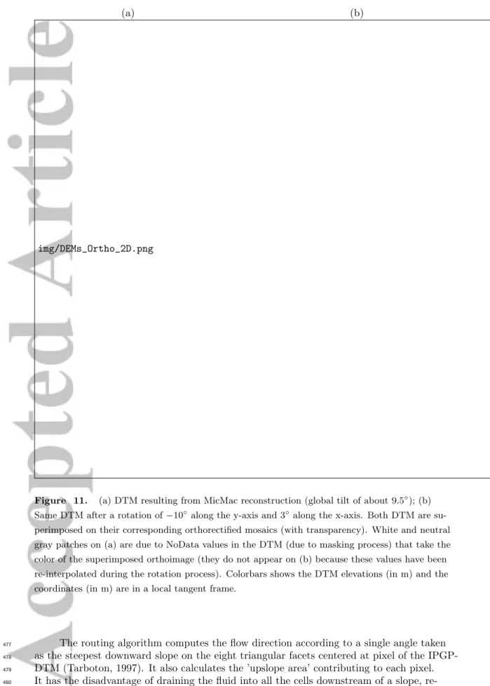
Figure 11. (a) DTM resulting from MicMac reconstruction (global tilt of about 9.5◦); (b) Same DTM after a rotation of −10◦along the y-axis and 3◦along the x-axis. Both DTM are su-perimposed on their corresponding orthorectified mosaics (with transparency). White and neutral gray patches on (a) are due to NoData values in the DTM (due to masking process) that take the color of the superimposed orthoimage (they do not appear on (b) because these values have been re-interpolated during the rotation process). Colorbars shows the DTM elevations (in m) and the coordinates (in m) are in a local tangent frame.
The routing algorithm computes the flow direction according to a single angle taken
477
as the steepest downward slope on the eight triangular facets centered at pixel of the
IPGP-478
DTM (Tarboton, 1997). It also calculates the ’upslope area’ contributing to each pixel.
479
It has the disadvantage of draining the fluid into all the cells downstream of a slope,
re-480
gardless of the slope inclination. In this way, the noise in the IPGP-DTM, which can cause
481
unrealistic altitude fluctuations, is treated as local minima by the routing algorithm and
can generate unrealistic flow routing. It is thus important to establish a minimum
thresh-483
old on the routing to ensure that fluids do not accumulate in these noisy regions and flow
484
in a more realistic way. This can be done by identifying an area of the DTM where the
485
routing algorithm leads to fluid accumulation when no rivers are observed and by
com-486
puting a threshold on the drainage area (i.e., a minimum number of drained cells) that
487
allows to eliminate these unrealistic fluid accumulations. Then we apply it to the whole
488
topography.
489
For each pair of rotation angles, a matching score is calculated as the percentage
490
of pixels determined by routing that match the actual rivers (Figure 12). The maximum
491
score is 62 %, for an optimal rotation angle of -10◦along the y-axis and 3◦ along the
x-492
axis (see Supplementary Information S6). Interestingly, it amounts to bringing the
IPGP-493
DTM back close to horizontal, with only a remaining gentle global slope and rivers
go-494
ing down the slope. Nevertheless this score should be interpreted carefully: it does not
495
mean that 62 % of the rivers has been rebuilt with the new IPGP-DTM. Indeed, the shorter
496
and stubbier rivers were not taken into account for this calculation and the network
cal-497
culated by the routing does not always follow the rivers continuously.
498
4 Results and discussion
499
The overall inclination and shape of the IPGP-DTM are consistent with the
ex-500
pected direction of the flow (L. A. Soderblom et al., 2007b). This is proved by the
rout-501
ing where the large rivers flow from the bright zone toward the dark area. Note that the
502
small rivers to the left of the scene, which were excluded from the score calculation, also
503
flow in the right direction from the highlands to the riverbed (see Figure 12 and
Sup-504
plementary Information S7).
505
However, some areas display a suspicious morphology. For instance the edges of
506
the IPGP-DTM, which we didn’t mask because of high correlation scores, are very steep.
507
Since such slopes (up to 80◦) are not observed on Earth at such small scales, the
accu-508
racy of the IPGP-DTM in these regions is questionable. Moreover, the routing does not
509
well match the rivers in these regions that display the highest EP values, in particular
510
the region for y<0 which is two to three time higher than in the center of the DTM
(Fig-511
ure 10). As a consequence, we advise users to always refer to the EP map when using
512
the IPGP-DTM.
513
The first improvement of the IPGP-DTM concerns the size of the reconstructed
514
region, which is larger than the USGS-DTM (10.3 km2 vs 7.5 km2) because we used more
515
images. The horizontal sampling of the IPGP-DTM is also better (18 m/px vs 50 m/px).
516
The flow direction on the topography of both DTM was calculated in the same way
517
using the TopoToolBox routine. Since they do not have the same size and resolution, we
518
cannot apply the same threshold for routing, nevertheless we applied the same method
519
to determine it. The resulting matching score is 35 % if we compute it on the original
520
USGS-DTM (L. A. Soderblom et al., 2007b). It is worth noting that, since the
orien-521
tation of the USGS-DTM was manually clipped to zero, we tried to find out if we could
522
find an optimal orientation as we did for the IPGP-DTM. Therefore, we rotated the
USGS-523
DTM in order to find the best matching score, as done with the IPGP-DTM, and found
524
a score of 56%. This score correspond to a rotation angle of 4◦ along the y-axis and 3◦
525
along the x-axis, which means that the global slope was underestimated, and by slightly
526
tilting the USGS-DTM, we find a more coherent configuration with regard to the shape
527
and location of the routing (see Supplementary Information Fig. S8). However, with this
528
rotation, the land at the bottom right of Fig. S4 is at the same elevation as the lakebed
529
at the bottom left, which is questionable.
530
If we consider the original USGS-DTM (no inclination) used in previous studies
531
(Tomasko et al., 2005; Jaumann et al., 2008; Tewelde et al., 2013), the routing shapes
(a) (b)
img/DEMs_3D.png
(c)
Figure 12. 3D views of the DTM: (a) IPGP-DTM (see also Supplementary Information S7), (b) USGS-DTM, and (c) IPGP-DTM with the footprint of the USGS-DTM (orange dashes). The vertical exaggeration is 1.5. The routing is superimposed (white line) on each DTM.
calculated from the two DTM are very different. The USGS-DTM provides a radial shape
533
routing while the IPGP-DTM provides a rather dendritic or rectangular shape.
Accord-534
ing to the literature (Perron et al., 2006; Burr et al., 2013) and even by simple visual
in-535
spection, the networks observed in our region of interest have dendritic or rectangular
536
shapes. As a consequence the IPGP-DTM seems to provide a better representation of
537
the local topography.
538
The last comparison consists in analyzing several river profiles and
transects/cross-539
sections in order to check if the inclination of the rivers is consistent with the
theoret-540
ical direction of flow and if the rivers, carved by liquid hydrocarbons, form depressions.
541
As far as the cross-sections are concerned, the river bottoms are generally located on flat
542
areas or in depressions for both DTM, except in a few cases where the rivers are located
543
on slopes (Figure 13). However, it is worth to note that, due to a coarser resolution, the
USGS-DTM has only one manual measurement point per river transect compared to an
545
average of three points for the IPGP-DTM. As for the river profiles, the flow of the main
546
river (profile C-C’ in green in Figure 13) follows the expected flow direction in the case
547
of the IPGP-DTM as opposed to the USGS-DTM, where the channel flows in the wrong
548
direction.
549
img/All_transects.png
Figure 13. Orthorectified mosaics calculated from (a) the IPGP-DTM and (b) the USGS-DTM. We display two cross-sectional profiles (c-d) and a profile along a river (e). The horizontal axis of the graphs represents the length of the transect and the vertical axis represents the alti-tude (in meters). The darker colours in each graph represent the cross-sections and follow-ups of the USGS-DTM while the lighter colours correspond to those of the IPGP-DTM. The dark red arrows refer to the valley bottoms visible on the orthorectified mosaics of USGS-DTM and the light red arrows correspond to those of our orthorectified mosaics. The two orthorectified images (and therefore the arrows) are offset because the topography of the two DTMs are not identical.
5 Conclusion
550
New investigation of the topography around the Huygens landing site has been
suc-551
cessfully carried out. We developed a new strategy that could overcome the high
com-552
plexity of the dataset, unusual even for planetary data, and provided a fully documented
553
and reproducible workflow. This procedure could be apply in situations with such a
com-554
plex dataset. For instance, it could be applied both to poorly known and hard-to-reach
terrestrial areas (i.e., Antarctica) and to archive data from former planetary missions (i.e.,
556
Voyager, Galileo, etc.). Besides a new strategy, the article provide a new DTM with a
557
higher spatial sampling and a more reliable topography since it is much less interpolated
558
than the previous product. This DTM offers new opportunities for investigating the
to-559
pography of fluvial landscape at Titan’s equatorial region with an unprecedented
res-560
olution. It could bring new insights on Titan’s landscape formation mechanisms by
quan-561
titatively characterizing the morphometry of these rivers and the topography of their
as-562
sociated drainage basins.
Appendix A Local Tangent Plane definition
564
The Local Tangent Plane (LTP) is an orthogonal, rectangular, reference system the
565
origin of which is defined at an arbitrary point on the planet surface (here we took the
566
nadir of the image #450 located at (167.64370◦E , −10.577749◦N)). Among the three
567
coordinates one represents the position along the northern axis, one along the local
east-568
ern axis, and the last one is the vertical position. If (λ, φ, h) are the coordinates of a
569
given point in the geographical frame, the coordinates (xt,yt,zt) of the LTP are defined 570 as: 571 xt yt zt = −sin(φ) cos(φ) 0
−cos(φ)sin(λ) −sin(λ)sin(φ) cos(λ) cos(λ)cos(φ) cos(λ)sin(φ) sin(λ)
· x − x0 y − y0 z − z0 with: 572
• (x, y, z) the Cartesian coordinates of the given point 573
• (x
0, y0, z0) the Cartesian coordinates of our reference point 574
Appendix B Dense pixel matching parameters
575
A sensitivity analysis has been performed on all the parameters of the dense pixel
576
matching step. The parameters selection was done manually, by changing their value in
577
order to keep most of the details while reducing the noise level. As observed on the
fig-578
ure B1, a smaller final resolution and a bigger quantification step and regularization
fac-579
tor tend to smooth the DMT and cannot detect the bottom of the rivers. On the
con-580
trary, a smaller size of correlation window tends to noise the DTM.
img/transect_comp_Malt.pdf
Figure B1. (a) Orthorectified mosaic calculated from the IPGP-DTM. We display the cross-sectional profile of the river (in orange on the orthoimage) and change the value of each param-eters for each panel. On every plot, the orange line represent the profile of the final DTM and the other line is the profile of the DTM with a different parameter (the unit for both axes is the meter): (b) the dark-blue line is the profile of the DTM for a smaller final resolution value, (c) the dark green plot for a smaller size correlation window, (d) the dark line correspond to a higher quantification step and (e) the blue plot is for a larger regularization factor. The dashed red line refer to the valley bottoms visible on the orthorectified mosaics of DTM.
Acknowledgments
582
The authors thank Chuck See for providing the re-processed DISR images. They also
583
thank the reviewers for their valuable comments and advice. MicMac software can be
584
downloaded for free (https://micmac.ensg.eu/index.php/Accueil) and the SPICE
ker-585
nels are publicly available (https://doi.org/10.5270/esa-ssem3np). The DTM and other
586
products resulting from this work are available on https://doi.org/10.5270/esa-3uja374.
587
References
588
Aharonson, O., Hayes, A. G., Lopes, R., Lucas, A., Hayne, P., & Perron, J. T.
589
(2014). Titan: Surface, atmosphere and magnetosphere. In (chap. Titan’s
590
Surface Geology). Cambridge University Press, pp. 43–75.
591
Archinal, B. A., Tomasko, M. G., Rizk, B., Soderblom, L. A., Kirk, R. L.,
592
Howington-Kraus, E., . . . Team, D. S. (2006). Photogrammetric Analysis
593
of Huygens DISR Images of Titan..
594
Atreya, S. K., Adams, E. Y., Niemann, H. B., Demick-Montelara, J. E., Owen,
595
T. C., Fulchignoni, M., . . . Wilson, E. H. (2006). Titan’s methane cycle.
596
Planetary and Space Science, 54 (12), 1177 - 1187.
597
Barnes, J. W., Brown, R. H., Soderblom, L. A., Buratti, B. J., Sotin, C., Rodriguez,
598
S., . . . Nicholson, P. D. (2007b). Global-scale surface spectral variations on
599
Titan seen from cassini/vims. Icarus, 186 (1), 242–258.
600
Barnes, J. W., Brown, R. H., Soderblom, L. A., Sotin, C., Le Mou`elic, S., Rodriguez,
601
S., . . . others (2008). Spectroscopy, morphometry, and photoclinometry of
602
Titan’s dunefields from cassini/vims. Icarus, 195 (1), 400–414.
603
Barnes, J. W., Radebaugh, J., Brown, R. H., Wall, S., Soderblom, L. A., Lunine,
604
J., et al. (2007a). Near-infrared spectral mapping of Titan’s mountains and
605
channels. Journal of Geophysical Research: Planets, 112 (E11).
606
Black, B. A., Perron, J. T., Burr, D. M., & Drummond, S. A. (2012). Estimating
607
erosional exhumation on Titan from drainage network morphology. Journal of
608
Geophysical Research: Planets, 117 (E8).
609
Bretar, F., Arab-Sedze, M., Champion, J., Pierrot-Deseilligny, M., Heggy, E., &
610
Jacquemoud, S. (2013). An advanced photogrammetric method to measure
611
surface roughness: Application to volcanic terrains in the Piton de la
Four-612
naise, Reunion Island. Remote Sensing of Environment, 135:1-11 .
613
Brossier, J. F., Rodriguez, S., Cornet, T., Lucas, A., Radebaugh, J., Maltagliati, L.,
614
. . . others (2018). Geological evolution of Titan’s equatorial regions:
possi-615
ble nature and origin of the dune material. Journal of Geophysical Research:
616
Planets, 123 (5), 1089–1112.
617
Burr, D. M., Emery, J. P., Lorenz, R. D., Collins, G. C., & Carling, P. A. (2006).
618
Sediment transport by liquid surficial flow: Application to Titan. Icarus,
619
181 (1), 235 - 242.
620
Burr, D. M., Perron, J. T., Lamb, M. P., Irwin III, R. P., Collins, G. C., Howard,
621
A. D., & Drummond, S. A. (2013). Fluvial features on Titan: Insights from
622
morphology and modeling. GSA Bulletin, 125 (3-4), 299-321.
623
Charles, H. A. (1996). Ancillary data services of nasa’s navigation and ancillary
in-624
formation facility. Planetary and Space Science, 44 (1), 65 - 70. (Planetary
625
data system) doi: https://doi.org/10.1016/0032-0633(95)00107-7
626
Collins, G. C. (2005). Relative rates of fluvial bedrock incision on Titan and Earth.
627
Geophysical Research Letters, 32 (22).
628
Cornet, T., Bourgeois, O., Le Moulic, S., Rodriguez, S., Lopez Gonzalez, T., Sotin,
629
C., . . . Nicholson, P. D. (2012). Geomorphological significance of ontario lacus
630
on Titan: Integrated interpretation of cassini vims, iss and radar data and
631
comparison with the etosha pan (namibia). Icarus, 218 (2), 788 - 806.
632
ESA SPICE Service. (2019). Huygens Operational SPICE Kernel Dataset.
633
doi: 10.5270/esa-ssem3np1