HAL Id: insu-02021644
https://hal-insu.archives-ouvertes.fr/insu-02021644
Submitted on 19 Jul 2020
HAL is a multi-disciplinary open access
archive for the deposit and dissemination of
sci-entific research documents, whether they are
pub-lished or not. The documents may come from
teaching and research institutions in France or
abroad, or from public or private research centers.
L’archive ouverte pluridisciplinaire HAL, est
destinée au dépôt et à la diffusion de documents
scientifiques de niveau recherche, publiés ou non,
émanant des établissements d’enseignement et de
recherche français ou étrangers, des laboratoires
publics ou privés.
Elisabeth Werner, E. Yordanova, A. P. Dimmock, M. Temmer
To cite this version:
Elisabeth Werner, E. Yordanova, A. P. Dimmock, M. Temmer. Modeling the multiple CME
inter-action event on 6-9 September 2017 with WSA-ENLIL+Cone. Space Weather: The International
Journal of Research and Applications, American Geophysical Union (AGU), 2019, 17 (2), pp.357-369.
�10.1029/2018SW001993�. �insu-02021644�
A. L. E. Werner1,2,3 , E. Yordanova1 , A. P. Dimmock1 , and M. Temmer4
1Swedish Institute of Space Physics, Uppsala, Sweden,2Department of Physics and Astronomy, Uppsala University, Uppsala, Sweden,3LATMOS/IPSL, Sorbonne Université, UVSQ, CNRS, Paris, France,4Institute of Physics, University of Graz, Graz, Austria
Abstract
A series of coronal mass ejections (CMEs) erupted from the same active region between 4–6 September 2017. Later, on 6–9 September, two interplanetary (IP) shocks reached L1, creating acomplex and geoeffective plasma structure. To understand the processes leading up to the formation of the two shocks, we model the CMEs with the Wang-Sheeley-Arge (WSA)-ENLIL+Cone model. The first two CMEs merged already in the solar corona driving the first IP shock. In IP space, another fast CME presumably interacted with the flank of the preceding CMEs and caused the second shock detected in situ. By introducing a customized density enhancement factor (dcld) in the WSA-ENLIL+Cone model based on coronagraph image observations, the predicted arrival time of the first IP shock was drastically improved. When the dcld factor was tested on a well-defined single CME event from 12 July 2012 the shock arrival time saw similar improvement. These results suggest that the proposed approach may be an alternative to improve the forecast for fast and simple CMEs. Further, the slowly decelerating kilometric type II radio burst confirms that the properties of the background solar wind have been preconditioned by the passage of the first IP shock. This likely caused the last CME to experience insignificant deceleration and led to the early arrival of the second IP shock. This result emphasizes the need to take preconditioning of the IP medium into account when making forecasts of CMEs erupting in quick succession.
1. Introduction
Coronal mass ejections (CMEs) are the main drivers of severe space weather and caused 87% of all intense (Dst ≤ 100 nT) geomagnetic storms between 1995 and 2014 (Shen et al., 2017). The main storm driving feature is a strong negative Bzmagnetic field component inherent to the magnetic flux rope embedded in
the plasmoid. Magnetic flux ropes marked by a high magnetic field strength, smooth rotation of one or two magnetic field components owing to the changing pitch angle in the flux rope (Burlaga, 1988), low proton temperatures (Richardson & Cane, 1995), and low magnetic field variance (Badruddin, 1998) are denoted as magnetic clouds (MCs).
CMEs frequently have their origin in active regions (ARs), which can be sufficiently energetic to support successive CME eruptions separated by a few hours to a few days, especially at the peak of the solar activity cycle. This provides the perfect conditions for CMEs to interact on their way to Earth and potentially form a strongly geoeffective structure. Already in the mid 1970s, it was noticed that CMEs might interact in the heliosphere (Intriligator, 1976). However, the first radio (Gopalswamy et al., 2001) and in situ observations (Burlaga et al., 2002) of interaction would have to wait until the early 2000s. At that time CMEs were thought to experience “CME cannibalism” and lose most characteristics of the original structures, the end product being a “complex ejecta.” These structures are most easily recognized by their weak and disordered magnetic field. There are also, other, very long duration events (Burlaga et al., 2002; Xie et al., 2006) characterized by a higher plasma beta than that of single MCs. A third type of multiple CME events has also been observed (Wang et al., 2003), in which distinct disjointed MCs can still be recognized (Wang et al., 2002).
A fast CME overtaking a slow preceding one would appear in the in situ observations as an enhancement of the magnetic field and Bzcomponent (if both MCs have similar orientation; Wang et al., 2003). These
events, called “shock-in-a-cloud,” are more likely to be geoeffective when Earth directed, since they also tend to result in a stronger geomagnetic response when compared to single, geoeffective CMEs (Lugaz et al., 2016). In fact, 30% of all intense geomagnetic storms in the study by Shen et al. (2017) were attributed to
Special Section:
Space Weather Events of 4-10 September 2017
Key Points:
• A series of CMEs from 4–6 September 2017 interacted and formed two IP shocks reaching Earth on 6–9 September
• The solar wind plasma was preconditioned by several merged CMEs from 4–5 September to exert little resistance against the 6 September CME
• We propose a new tool with potential to greatly improve the arrival time prediction for fast single halo CMEs
Supporting Information: • Supporting Information S1 • Movie S1 Correspondence to: A. L. E. Werner, [email protected] Citation:
Werner, A. L. E., Yordanova, E., Dim-mock, A. P., Temmer, M. (2019). Modeling the multiple CME inter-action event on 6–9 September 2017 with WSA-ENLIL+Cone. Space
Weather, 17, 357–369. https://doi.org/ 10.1029/2018SW001993
Received 29 JUN 2018 Accepted 13 FEB 2019
Accepted article online 14 FEB 2019 Published online 27 FEB 2019 Corrected 31 JUL 2019
This article was corrected on 31 JUL 2019. See the end of the full text for details.
©2019. American Geophysical Union. All Rights Reserved.
shock-embedded CMEs. Simulations of shock-in-a-cloud events confirm the overall picture predicted from theory: compression of the magnetic cloud in the radial direction, elevated magnetic field, and temperature spikes (Lugaz et al., 2005; Vandas et al., 1997; Xiong et al., 2006).
Despite being in the declining phase of the current solar cycle, the time period between 4 and 10 September 2017 was marked as a time of strong solar activity and saw several instances of strong, geoeffective events, all of which had their origin in the rapidly evolving active region NOAA AR 12673. Much attention has been devoted to the solar energetic particle (SEP) impact on Mars from the X8.2 class flare on 10 September (e.g., Guo et al., 2018; Harada et al., 2018; Luhmann et al., 2018). Here, we consider the earlier series of CME eruptions which took place between 4 and 6 September. There are indications that these CMEs have interacted during their propagation into interplanetary (IP) space, resulting in a complex transient detected at L1 in the period 6–9 September, and the geomagnetic storm on 8 and 9 September.
Multiple CME interaction events such as this one are particularly difficult to forecast. The predictions posted on the CME Scoreboard (developed at the Community Coordinated Modeling Center; CCMC) for the most geoeffective CME on 6 September, created with a variety of different models, overpredicted the time of arrival with +7.5 up to +23.5 hr. For reference, the mean absolute error for the Wang-Sheeley-Arge (WSA)-ENLIL+Cone model has been estimated to 10.4 ± 0.9 hr. This estimation was determined in a sta-tistical study of over 1,800 CME events modeled with the WSA-ENLIL+Cone model (Wold et al., 2018). In analogy, only one model estimated the correct geomagnetic response of the CME which erupted on 6 September (max Kp = 8.0). The predictions for the CME events on 4 September saw the opposite trend; the corresponding IP shock arrived somewhat later than anticipated and triggered a weaker geomagnetic response. The results from these forecasts suggest that this event is very complex. As such, this period of solar activity may provide a good “baseline” event for probing the geoeffectiveness of interacting CMEs. The objective of this case study is to test the performance of the WSA-ENLIL+Cone model for this type of complex events. There have been numerous validation efforts made in the past for single CME events (Falkenberg et al., 2010; Mays et al., 2015; Xie et al., 2013). We introduce various modifications to the input and evaluate their influence on the fit of the forecast. Special care has been taken to apply changes to the input which are driven from observations and which are well suited for an operational setting. The paper is organized as follows: Section 2 describes the event in detail based on the available coronagraph and in situ observations. Section 3 describes the method used to determine the CME kinematics and shock propagation. The results of the model runs are presented in section 4. The findings and their implications for the event under study and CME forecasting, in general, are discussed in section 5 and summarized in section 6.
2. Event Overview
In this section we describe the coronagraph observations of the series of CMEs that may have led to the formation of the complex transient detected at L1 on 6–9 September 2017. We also present an overview of the respective in situ and radio wave observations made by the WIND spacecraft. The CME speeds provided below (see also Table 1) were obtained with the method described in section 3.
CME 1 made its first appearance at the inner boundary of the Solar and Heliospheric Observatory (SOHO)/Large Angle and Spectrometric Coronagraph (LASCO)/C2 on 4 September, 19:00 UTC. This CME, along with the following three CMEs, can be traced back to AR 12673 which at this time was located at S10W14 (Stonyhurst heliographic coordinates). Its direction of motion had a strong component toward the southwest as seen from SOHO/LASCO, and the presumed eruption time of CME 1 is roughly concurrent with a M1.7 class flare (S09W11) with start time 18:46 UTC. CME 1 can be classified as a partial halo CME. The CME maintained a moderate speed of approximately 710 km/s until it was overtaken by the second, much faster CME 2.
The CME 2, which was faster (1,350 km/s), first appeared in SOHO/LASCO/C2 at 20:36 UTC and envelops the previous CME 1 by 21:18 UTC. This CME was concurrent (20:28 UTC) with a M5.5 class flare located at S10W11. In contrast with the previous CME 1, CME 2 quickly developed halo CME characteristics and white-light shock observed by SOHO/LASCO/C3.
At 17:36 UTC on the following day (5 September) another partial halo CME appeared in the field of view of SOHO/LASCO/C2. Active region AR 12673 was located at S08W28 at this time, and an M2.3 class flare with the position S10W23 erupted at 17:37 UTC. This CME had only weak white-light signatures in the
Table 1
Input Parameters for the Selected Events in the Baseline and Custom Run Baseline run: CME: 1 2 3 Time @21.5R⊙ 2017-9-4 23:41 2017-9-4 22:36 2017-9-6 14:13 Latitude −6◦ −18◦ −12◦ Longitude 28◦ 22◦ 32◦ Half-width 18◦ 42◦ 46◦ Speed @21.5R⊙ 710 km/s 1350 km/s 1480 km/s Custom run: dcld - 2.1 1.2
Note. The custom run only includes CMEs 2 and 3.
coronagraph data and the leading edge could not be followed past 5R⊙. For this reason we do not model this CME. Shortly thereafter, at 18:03 UTC, a fast narrow CME was propagating along the westward streamer in SOHO/LASCO/C2. This CME was unlikely to be Earth directed.
CME 3, first appearance in SOHO/LASCO/C2 at 6 September 12:24 UTC, is the last CME in this series, most likely contributing to the complex ejecta later detected in situ. It reached a velocity of 1,480 km/s, surpassing the speed of all previous CMEs. This CME appeared as an asymmetrical halo with a large angular extent in the SOHO/LASCO field of view. This CME also had its source in AR 12673 (now located at S09W42) and its eruption was concurrent with an X9.3 class flare (11:53 UTC) at S09W34.
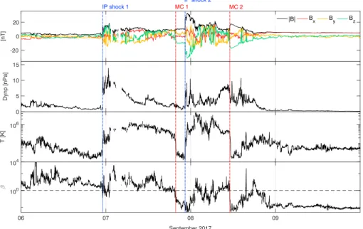
CME 1 and CME 2 merged into a single structure already in the lower corona, forming the single IP shock reaching L1 at 23:05 UTC on 6 September (see Figure 1). From here on in the paper this shock will be referred as IP shock 1. This shock was immediately followed by a prolonged sheath region as characterized by a turbulent behavior of the magnetic field components, enhanced plasma temperature, and dynamic pressure (Figure 1).
Figure 1. The 1-min averaged magnetic field and plasma data as detected by WIND at L1. The first panel (top to
bottom) displays all magnetic field components in the geocentric solar magnetospheric system and|B|. The second panel shows the dynamical pressure, the third the proton temperature, and the fourth panel displays the plasma𝛽 ratio. The dashed horizontal line in panel 4 marks the𝛽 = 1line, which enables the identification of dominant magnetic structures (i.e., magnetic clouds; MCs). The dotted vertical lines across all panels signifies the arrival of interplanetary (IP) shocks 1 and 2 (blue), while the vertical lines in red represent the arrivals of MCs 1 and 2.
On 7 September at 19:45 UTC, the plasma𝛽 (the ratio between plasma and magnetic pressure) dropped below 1. This was accompanied by a drop in the proton temperature by almost 2 orders of magnitude, related to the reduced thermal pressure. The in situ observations indicate the arrival of a magnetic cloud likely associated with the merged CMEs and will be referred throughout the paper as MC 1. Low plasma beta and proton temperature, and smooth magnetic field, are typical characteristics of magnetic clouds. The absence of clear rotation in MC1 implies that the spacecraft trajectory is probably passing through the edge of the cloud (Kim et al., 2013).
On 7 September 22:27 UTC another IP shock (IP shock 2) arrived, which is most likely the result of the fast asymmetrical halo CME from 6 September (CME 3 described above). Behind IP shock 2 followed another turbulent sheath region and at 11:10 UTC on 8 September arrived the magnetic cloud associated with CME 3, which will be called MC 2 further on. While the leading edge of MC 2 is well seen in the in situ data, it is difficult to identify its trailing edge. In the period 14:00–16:00 UTC on 8 September, polarity changes in all magnetic field components associated with𝛽 > 1 can be clearly seen. After that, however, 𝛽 reveals the characteristic of a magnetic structure with very low and weakly fluctuating values. Also, the magnetic field components show no clear rotation and are oriented along the Sun-Earth line, suggesting that the spacecraft trajectory may be aligned with the axial field of MC 2. Therefore, we can speculate that the MC 2 encounter continued at least until midnight on 9 September.
The arrival of IP shock 2 was marked as a steep drop of Bzcomponent at 22:27 UTC on 7 September, which triggered an intense geomagnetic storm (Dst < −100 nT). We argue that the unexpectedly strong geomag-netic response was likely caused by the plasma compression due to the propagation of the IP shock 2 inside MC 1. This can be seen as the increase in the dynamic pressure and the temperature spike at the shock (Figure 1, panels 2 and 3). Such shock-in-a-cloud configuration has been reported in Lugaz et al. (2015). The duration of MC 1 is very short, despite that,𝛽 remains below 1 until 01:18 UTC on 8 September. This suggests that MC 1 had merely a flank encounter with Earth. The relatively small temperature spike at the shock would imply that the IP shock 2 has not progressed very far into MC 1, which is also confirmed by the weak dynamic pressure of the event.
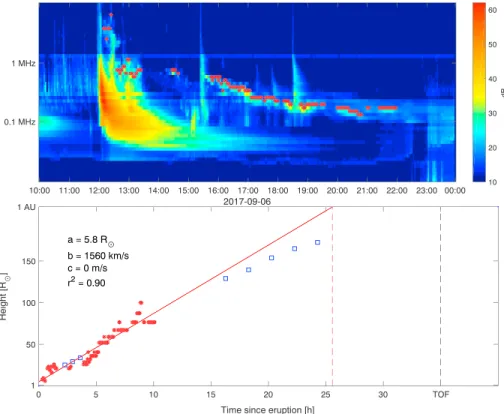
The eruption of the 6 September CME (CME 3) was followed by a type II radio burst, as detected by WIND/WAVES experiment (see Figure 2). The occurrence of a type II radio burst is indicative of shock propagation through the solar corona and IP medium (Reiner et al., 1998). The emission starts shortly after the eruption (12:10 UTC) in the metric and decameter-hectometric (DH) range, moving further into the kilometric range at 15:00 UTC until the arrival of IP shock 1 at L1 (6 September, 23:00 UTC; see Figure 2, top panel).
3. Method
3.1. Determination of CME Kinematics
In this study we use runs from the WSA-ENLIL+Cone model, which is a coupled model consisting of the semiempirical WSA coronal model, the geometric Cone model and the magnetohydrodynamical (MHD) model ENLIL. WSA and Cone provide the inner boundary conditions to ENLIL, which is then capable of describing the propagation of a CME through the heliosphere and enables its tracking in three dimensions from the inner boundary at 21.5R⊙up to a distance of 10 AU. WSA-ENLIL+Cone is publicly available for simulation runs by CCMC (http://ccmc.gsfc.nasa.gov).
We used the synoptic magnetogram by Synoptic Optical Long-term Investigation of the Sun (SOLIS) at Kitt Peak Observatory for Carrington rotation 2194 as input to the WSA model. The Global Oscillation Network Group (GONG) is the typical choice of magnetogram provider, but the representation of the polar fields in our initial runs, obtained using GONG magnetograms, was not accurate enough (see section 5 for further discussion). Synoptic magnetograms from the Mount Wilson Observatory (MWO) were not available at the time for the relevant Carrington rotation.
The input CME parameters (radial speed, cone angular width, and propagation orientation) to the Cone model are determined using simultaneous coronagraph images from two different viewpoints. Corona-graphs view the electron scattering efficiency produced from Thompson scattering rather than the actual radiated light from the corona. This means that the viewing angle of the observer will have a considerable effect on the imaged coronal structure, as the scattering efficiency quickly falls off from its maximum at 90◦(i.e., in the plane-of-sky) to only a few percent at 60◦(Hundhausen, 1993). This in turn implies that the
Figure 2. (top) Dynamical spectra of the radio emission following CME 3 from 6 September, selected data points (red
asterisks), and (bottom) the resulting propagation profile and fit. The fit is compared with distance-time data points from Solar Terrestrial Relations Observatory (STEREO-A)/Sun-Earth Connection Coronal and Heliospheric Investigation (SECCHI)/Heliospheric Imager (HI) white-light shock observations (blue squares), which have been derived from J-maps. The dashed red line in the bottom panel marks the estimated time of arrival from the fit, while the black line marks the true time of arrival (TOF) of IP shock 2.
true leading edge of an Earth-directed CME will be practically invisible to a coronagraph situated at L1 (i.e., SOHO). Using the geometric triangulation method (Liu et al., 2010) in such a case, will lead to large errors not only in the estimated radial speed but also the width and direction of motion, rendering this technique unsuitable for full, partial or asymmetric halo CMEs. It is possible however to estimate the true radial speed from the plane-of-sky speed.
First, imagine an idealized halo CME scenario, that is, the CME's direction of motion being perfectly orthog-onal to the plane of sky as seen by the coronagraph. What is viewed then is not the radial speed vr, but rather the expansion speed vexp(or more correctly vdisk=
1
2vexp, where vdiskis centered at the solar disk, see
Figure 3. Schematic showing the line-of-sight view for a cone coronal mass
ejection erupting on the limb (a) and a halo coronal mass ejection (b). Figure adapted from Gopalswamy et al. (2009).
Figure 3). Furthermore, assuming that the CME in question follows the postulates given by the Cone model, the expansion speed at any cut will closely resemble that of the leading edge. Gopalswamy et al. (2009) could show from observations that vr ≈ 1
2vexp, giving at last the very conve-nient conclusion that vr≈vdiskfor very fast (vr≈1,000 km/s) and wide
(𝜔 ≈ 45◦) CMEs. This relationship was also found in a more recent and larger statistical study (Jang et al., 2016). Thus, it will suffice to estimate
vdisk, which may be done in the frameseries mode in StereoCAT (LaSota, 2013). This mode allows for tracking of the leading edge across several frames. However, it has been shown (Dal Lago et al., 2003) that even for perfect halo CMEs vris not necessarily similar to vexp. The true direction of motion will likely lie somewhere between the plane of sky and the line of sight. This means that the plane-of-sky speed will include a contribu-tion from both vLE = vrand vdisk = 1∕2vexp = vr, meaning that the estimated speed will be higher than the true vr. Therefore, if the objective
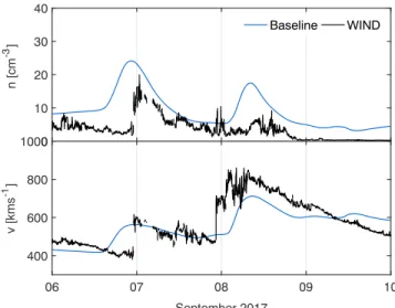
Figure 4. Output at L1 from the WSA-ENLIL+Cone baseline run and
WIND data.
is to get the most reliable estimate of vdisk, then the plane-of-sky speed of the merged CME on 4 September is preferentially measured from SOHO, and from Solar Terrestrial Relations Observatory (STEREO-A) for CME 3. The speeds are estimated at 1,380 km/s for CME 2 and 1,470 km/s for CME 3 (Table 1).
The described method is limited to estimating the true radial speed of the CMEs and cannot provide other necessary input to the Cone model, such as the width and direction of motion. For this it is preferable to use a forward-modeling technique such as the Graduated Cylindrical Shell (GCS) model proposed by (Thernisien et al., 2006; Thernisien, 2011), which will also provide some realism to the plane-of-sky speeds estimated in StereoCAT. The GCS model consists of two conical legs attached to a curved cylindrical front, which can be fully described with the follow-ing three variables: (1) the height of the legs h; (2) the aspect ratio𝜅, which relates h to the angular width of the legs; and (3) the half angle
𝛼, measured from the full GCS symmetry axis (i.e., radial) to the
sym-metry axis of the legs. Then, we use the IDL/Solarsoft interface to fit the projected GCS model with difference images from the viewpoints of STEREO-A/Sun-Earth Connection Coronal and Heliospheric Investiga-tion (SECCHI)/COR-2 and SOHO/LASCO/C2 and C3. The GCS input variables, as given in Table 1, make up the baseline run. The speed estimates in Table 1 were determined from GCS fit heights at a 36- to 60-min time separation as close to the 21.5 R⊙height limit as possible and is assumed to follow a linear speed pro-file. In Figure 4 we compare the output solar wind proton number density and bulk plasma velocity from the baseline run with 1-min average WIND measurements from NASA/GSFC's CDAWeb, which will be addressed in detail in section 4.
3.2. IP Shock Propagation From Type II Radio Burst
Type II radio burst emission can be used to track the CME-driven shock wave propagation through IP space. We follow the main methodology described in Cremades et al. (2015) and focus our attention to the emission around and below 1 MHz to be consistent with their study. First, the type II radio emission is isolated from the rest of the spectra to avoid contamination by type III bursts. In this subportion of the full dynamical spectrum, the frequency with the strongest emission at every time step is selected to represent the central frequency. The central frequencies are converted to distances using a coronal electron density model. Unlike Cremades et al. (2015), who used the Leblanc et al. (1998) model, we use the Vršnak et al. (2004) hybrid model. This model combines a fivefold Saito et al. (1970, 1977) model, suitable for the equatorial corona with the Leblanc et al. (1998) model, which performs well at large distances from the Sun (i.e., IP space). Since we will be including a few data points just above 1 MHz at DH frequencies, this is the most appropriate choice. The frequency-time drift at kilometric wavelengths of the 6 September type II radio burst is located between 0.6 MHz and 40 kHz (see Figure 2). Emission in this frequency range mainly probes the IP medium (1 MHz to 30 kHz corresponds to 10–20 R⊙—1 AU). At these distances from the Sun the ambient solar wind gains influence, causing all CMEs to revert to a gradual deceleration/acceleration (Liu et al., 2013). The fit gives an approximate value for the shock distance, speed, and acceleration. Since CME 3 is rather fast (1,480 km/s), it is expected that the frequency-time drift of the type II burst should reflect a moderate deceleration. The eruption of CMEs 1 and 2 (4 September) were also accompanied by a type II radio burst, beginning with some decametric to hectometric emission at 20:35–21:40 UTC (WAVES/RAD2) and kilometric emission from 22:10 UTC and onward (WAVES/RAD1). However, the weak emission (< 20 dB) in the kilometric range and the commencement of a type III radio burst storm from 01:30 UTC on 5 September produced unfavorable conditions to determine a propagation profile for what is, presumably, IP shock 1.
4. Results
Figure 4 depicts the output of WSA-ENLIL+Cone at L1 for the modeled number density (top panel) and flow speed (bottom panel), compared to 1-min averages of the proton number density and bulk plasma speed
Figure 5. The radial solar wind velocity output from the baseline run as
shown in the ecliptic plane. This snapshot from 7 September 18:00 UTC illustrates the longitudinal extent of all three coronal mass ejections (CMEs). See also Figure 4 for the output at L1. The full video is available in the HTML version of this paper or in the supporting information S1.
measured by WIND. A first glance at Figure 4 reveals that there are two main issues with the baseline run: (1) the early arrival of IP shock 1, and (2) the high-density amplitude of both IP shocks. The baseline model pre-dicts an arrival time of IP shock 1 which lies 7.5 hr ahead of the true arrival time. The arrival time of IP shock 2 is instead overestimated by 4 hr. The density is overestimated by 43% for IP shock 1 and 220% for IP shock 2. The difference in the speed is about 8% for IP shock 1 and has been underestimated by 18% for IP shock 2.
Figure 5 depicts the speed output of the baseline model in the ecliptic plane at a point in time when all CMEs can be distinguished from the background solar wind. CME 1 and CME 2 merged before reaching the inner boundary of ENLIL and so are viewed as a single shock. Neither of the CMEs had a direct hit with Earth but rather a flank encounter. What is not shown in this figure is that the same holds in the meridional plane, that only the top portion of CMEs 1–3 reach Earth. This explains the large difference between the modeled and observed IP shocks in Figure 4. In an attempt to improve the forecast, a number of alterations were introduced to the input. The most fruitful experiment came about from introducing a change in one of the standard cone enhancement factors, more specif-ically the density enhancement factor (dcld). We will reflect briefly on how this feature can be determined from coronagraph images, and the interesting effects it has on the prediction for the first IP shock when introduced in the baseline run.
Dcldrefers to the density enhancement of the leading front of the CME cone relative to the density of the fast, ambient solar wind and is usually set to a value of dcld = 4. Falkenberg et al. (2010) did a parameter study with an earlier version of the WSA-ENLIL+Cone model, and found that a higher dcld factor results in a higher amplitude and earlier shock arrival at L1. The dcld factor gauges the mass of the CME, and so with a higher value one would expect less extensive drag from the ambient solar wind, hence the earlier arrival. It is interesting to note that lowering the dcld factor for our event could potentially serve to both remedy the too high amplitude and too early arrival of IP shock 1 in the baseline run. Scolini et al. (2018) have also achieved better predictions with the WSA-ENLIL+Cone model for two multiple CME
Figure 6. The dcld cuts (left) taken along the dashed white line (right). The input to WSA-ENLIL+Cone has been
taken as the ratio between the intensity of the shock front, as marked by the red arrow (left) and the ambient solar wind. The blue arrow (left) and the dashed blue curve (right) marks the CME driving the shock (“Driver”).
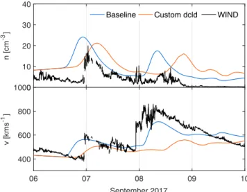
Figure 7. Output from the WSA-ENLIL+Cone model custom run
compared to the baseline run and WIND data.
events after replacing the standard dcld value with dcld = 2. A recent study on the shock compression factor of halo CMEs (Kwon & Vourlidas, 2018) indicated that dcld could take a range of values between 1.3 and 4.8. Therefore, introducing a change in the dcld factor is well warranted. We used an image from LASCO/C3 around the time when the actual front crossed the inner boundary at ∼21.5 R⊙to make a cut across the leading edge of the CME. The density enhancement compared to the ambient solar wind can then be estimated from the relative change in the image pixel count (see Figure 6). To increase the signal-to-noise ratio several cuts were made at approximately the same location. The dcld factor of CME 1 could not be reliably estimated as CME 2 merged with CME 1 before reaching 21.5 R⊙. Therefore, only CMEs 2 and 3 were included in the custom run in order to reduce the number of uncertain parameters (see Table 1).
When these custom dcld factors are introduced into the original run, the forecast for the IP shock 1 drastically improved (see Figure 7). The differ-ence between the estimated and the true time of arrival has been reduced from +7.5 to +1.3 hr, in this case. Note, however, that it nearly removed the second shock feature and increased the time lag to a total of +14 hr. A possible explanation for the late arrival would be a change in the ambient solar wind conditions. But if fast, tenuous solar wind was left in the wake of IP shock 1, as predicted by Temmer et al. (2017), the shock front would experience less drag from the surrounding environment and could maintain a higher speed, result-ing in the earlier arrival at L1. This would also serve to lower the density readout and increase the speed of the shock, both are needed to improve the run.
We also investigated the type II radio burst emission to obtain the velocity profile of IP shock 2. The dynamic spectrum of the radio emission and the data points (red asterisks) used for the fit are shown in the top panel of Figure 2. The bottom panel presents the speed profile, fitted to the second harmonic of the radio emission (red asterisks). From the fit we obtain the shock height a, initial velocity b, accelera-tion c, and the correlaaccelera-tion coefficient of the fit r2. By comparing the fit with distance-time data points from STEREO-A/SECCHI/Heliospheric Imager (HI) white-light shock observations which have been derived from J-maps (blue squares), we were able to determine that the emission is emitted at the second harmonic. STEREO-A had a position angle of roughly East 130◦(−128.2◦) at the time of the observations, that is, at a 155◦separation angle in longitude with CME 3. The two vertical dashed lines in Figure 2 marks the esti-mated time of arrival (red) extrapolated from the fit and the true arrival (black) of the shock at L1. Note that the fit gives an earlier arrival time for the IP shock 2 (25.6 hr after eruption), suggesting a possible interaction between the CMEs from 4 and 6 September.
5. Discussion
As mentioned in the event overview, we only include the CMEs from 4 and 6 September in the WSA-ENLIL+Cone model runs. It would seem that the CME which erupted on 5 September could have similar characteristics to the modeled CMEs 1-3. The position angle of the southern flank and that it likely originates from the same active region would make it appear to have a similar width and direction of motion as the other CMEs. What sets it apart from CMEs 1–3, is that it has very weak white-light signatures. As they all appear to have a similar direction of motion, Thompson scattering would be expected to have similar influence on all CMEs and presumably could not be the sole cause for the weak appearance of this particular CME. This would suggest that the CME on 5 September 5 is of low density and therefore vanished quickly in the white-light data. The SOHO LASCO CME catalog gives a speed estimate of 474 km/s for this CME, which would make it considerably slower compared to the other CMEs. Thus, because of its low speed and density we do not expect a shock from this CME at Earth. However, it is possible that the 5 September CME could contribute to the preexisting southward magnetic field ahead of IP shock 2 and in such a way enhances the geoeffectiveness of this event (Liu et al., 2016).
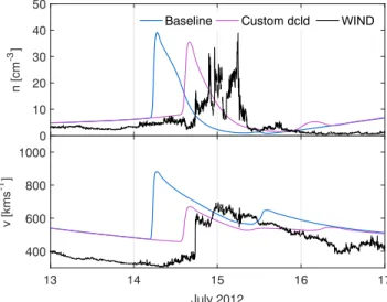
Figure 8. Baseline and custom dcld output from the WSA-ENLIL+Cone
model and WIND data for the 12 July 2012 coronal mass ejection event.
In a comparative study by Jian et al. (2015) it was shown that runs with both WSA(-ENLIL) and MHD-Around-a-Sphere model (MAS) using GONG magnetograms are able to represent best the speed patterns of the fast and slow solar wind. However, the use of GONG magnetograms which have not been zero-point corrected in model runs intended for forecasts may give rise to large errors in the time of arrival. Uncorrected GONG maps are more likely to have unbalanced magnetic flux, which can manifest itself as one pole being stronger than the other (G. Petrie, per-sonal communication, 2018-11-21). This is something we encountered in our initial runs (not shown), where the south pole coronal hole exhibited a very small latitudinal extent compared to the polar coronal hole in the north. As a result, the properties of the slow solar wind stream (through which all of the three CMEs are propagating) are greatly enhanced (larger angular extent, higher density). The pileup and greater resistance from the ambient medium caused IP shock 1 to arrive ∼7 hr later than in our baseline run with the Kitt Peak/SOLIS magnetogram, and the density to reach an amplitude of up to 40 cm−3at the shock front. Such modulation of CME properties by the ambient solar wind was also discussed in Riley et al. (2018). However, IP shock 2 was not as strongly affected as IP shock 1. This is due to the fact that the first IP shock propagates through an undisturbed medium, while IP shock 2 encounters the wake of the first IP shock and so is much less influ-enced by the choice of magnetogram. For this reason we encourage the use of zero-point corrected GONG magnetograms in future studies, which currently can be made per special request from the CCMC. The cor-rected GONG maps can also be accessed directly from the GONG archive at https://gong2.nso.edu/archive/ patch.pl?menutype=z.
We applied the same custom dcld extraction procedure to the well-defined single CME event from 12 July 2012, which produced an unusually long-lasting geomagnetic storm (Baker et al., 2013; Hu et al., 2016). This CME was fast (1,530 km/s) and its path through IP space was free of any previous CMEs up to 7 days prior. The WSA-ENLIL model prediction of the shock arrival time saw a great improvement, just as in the case of IP shock 1 in the September 2017 event (see Figure 8). The difference between the estimated and the true time of arrival has been reduced from 12.5 to 4 hr, and the speed amplitude from 40% to 7%. This result indicates that the custom dcld feature could potentially offer a quick, simple, and accessible way of improving the forecast for “undisturbed” events, that is, when there are no previous (∼2–5 days prior) Earth-directed, geoeffective events (Temmer et al., 2017). Such a relationship would have to be investigated in more detail in a future study by testing it against a statistically significant set of CMEs.
The proposed method to determine the dcld feature is simple and fast to implement, which should make it useful in an operational setting. We recognize however that this method is better suited to give a proxy rather than a true representation of the density enhancement at the actual shock front. If the density distribution along the line of sight is not taken into account, the estimate is likely to suffer from projection effects due to Thompson scattering. Our estimates are in line with previous work on estimating the density enhancement factor (Kwon & Vourlidas, 2018; Ontiveros & Vourlidas, 2009; Susino et al., 2015). The methodology recently presented by Kwon and Vourlidas (2018), who used a forward model to estimate the shock compression at the true shock front, is especially promising.
Determining the input parameters is acknowledged as one of the most difficult aspects of forecasting, and triangulation of the direction of motion, speed, and true cone half-width is not always accessible at any time or any geometry of a particular event. What this study suggests is that the plane-of-sky speed may offer a viable alternative to a triangulation procedure for halo CMEs or for CMEs with a direction of motion (or source region) at a 180◦angle from another field of view (STEREO-A).
The conclusion in section 4 regarding the type II radio emission being emitted at the second harmonic rests on the assumption that the source position of the type II radio emission is close to the CME nose. This is not necessarily the case, as many type II radio bursts have been reported to originate from the CME flank (e.g., Feng et al., 2013; Krupar et al., 2016; Magdaleni ´c et al., 2014; Shen et al., 2013; Xie et al., 2012). Mäkelä et al. (2018) were able to locate the radio emission source of the 6 July 2012 CME to the CME nose using radio
Figure 9. The average acceleration of 71 coronal mass ejections (CMEs) as a function of their initial speed, inferred
from kilometric type II radio burst emission. The star symbol marks the propagation profile of CME 3 in this study, and the encircled data points mark events with similar characteristics. Plot adapted from Cremades et al. (2015) by permission from Springer Nature.
direction-finding analysis, indicating that this might be the case for a few selected events. In Biesecker et al. (2002) it is discussed that the type II radio emission may be predominantly harmonic for CMEs erupting close to the solar limb. Biesecker et al. (2002) also refer to a study by Švestka and Fritzová-Švestková (1974), in which they found that the second harmonic of the type II radio bursts may be experiencing a maximum close to W40/E40. We believe that this might be the case for our event considering that AR 12673 was located at S09W42 on 6 September.
From the fit parameters of the type II radio burst, listed in Figure 2, it is clear that CME 3 propagates with nearly constant speed. The small deceleration indicates that the ambient solar wind conditions in the wake of the previous IP shock 1, have been altered to exert very little resistance against CME 3. Other events with similar characteristics have been previously reported by Liu et al. (2014) and Temmer and Nitta (2015). The fit has not been constrained to the true arrival time of IP shock 2 and is thus limited to describing the IP propagation profile of CME 3 up to ∼100 R⊙. The discrepancy between the arrival time extrapolated from the fit and the actual shock arrival time implies that the deceleration could be associated with the interaction between MC 1 and IP shock 2.
Figure 9 shows the average acceleration against the initial speed of the 71 CMEs included in the Cremades et al. (2015) study. The propagation profile of CME 3 (star symbol) lies at the edge of this distribution. While all CMEs with initial speeds>1,500 km/s appear to be decelerating, there are a few points clus-tered around CME 3 with similar speeds and linear propagation profiles (see circled points in Figure 9). These events all turn out to have another feature in common with CME 3, namely, that they are all pre-ceded by 1–3 high-speed CMEs with roughly the same direction of propagation appearing within ∼2–4 days from the eruption of the main CME. This implies that the propagation profile of CME 3 is typical for a preconditioned CME.
6. Conclusions
We study the interaction of ejecta from 4–6 September 2017. Their resulting complex structure was observed in situ at L1 on 6–9 September. One of the most prominent signatures seen in the in situ data is the shock-in-a-cloud structure that was produced as the IP shock of the fast CME from 6 September, interacted with the flank of the flux rope that likely resulted from the merging of the two CMEs from 4 September. We attempt to create a coherent picture of the CME merging process by linking coronographic imaging
observations, in situ measurements, and long wavelength radio observations with modeling of the CMEs' propagation in the inner heliosphere. We model these three CMEs with the WSA-ENLIL+Cone model. The introduction of the custom density enhancement (dcld) feature resulted in a considerable improvement of the time of arrival for IP shock 1. The successful test on a single halo CME event (12 July 2012) seems to indicate that this technique could have more widespread applicability, by offering a quick, easy, and suc-cessful way of improving the forecast for fast, undisturbed CMEs. This technique, however, did not have the same advantageous effect on the prediction of the amplitude and arrival time of IP shock 2. If the properties of the plasma have been preconditioned by the passage of the previous IP shock 1, one would expect an early arrival of IP shock 2. This implies that the magnetic effects arising from shock-flux rope interactions, which cannot be reproduced with WSA-ENLIL+Cone, may account for the discrepancy in the shock arrival time and the enhanced geoffectiveness of the combined structure. Clearly, more attention should be devoted to modeling in the future of CME-CME merging and their interaction in IP space with realistic background solar wind.
The analysis of the type II radio burst emission following the eruption of CME 3 suggests that the properties of the solar wind in the wake of IP shock 1 were indeed altered to exert very little resistance against the propagation of CME 3. This is evident from the nearly constant speed of both CME 3 and the associated shock wave during their propagation into IP space. Clearly, the preconditioning of the solar wind allows for the advance of subsequent IP shocks. In addition, this can lead to greater geoeffectiveness, in cases where an IP shock propagates into a preceding CME and compresses the magnetic cloud, as exemplified by Liu et al. (2014).
In summary, this study proposes means for improving the modeling: (1) of fast undisturbed CMEs by intro-ducing a custom density enhancement (dcld); and (2) of complex ejecta, resulting from interacting CMEs and the accompanied preconditioning of the IP solar wind, by using radio wave observations.
References
Badruddin, M. F. (1998). Interplanetary shocks, magnetic clouds, stream interfaces and resulting geomagnetic disturbances. Planetary and
Space Science, 46, 1015–1028. https://doi.org/10.1016/S0032-0633(98)00031-2
Baker, D. N., Li, X., Pulkkinen, A., Ngwira, C. M., Mays, M. L., Galvin, A. B., & Simunac, K. D. C. (2013). A major solar eruptive event in July 2012: Defining extreme space weather scenarios. Space Weather, 11, 585–591. https://doi.org/10.1002/swe.20097
Biesecker, D. A., Myers, D. C., Thompson, B. J., Hammer, D. M., & Vourlidas, A. (2002). Solar phenomena associated with “EIT waves”.
The Astrophysical Journal, 569, 1009–1015. https://doi.org/10.1086/339402
Burlaga, L. F. (1988). Magnetic clouds and force-free fields with constant alpha. Journal of Geophysical Research, 93, 7217–7224. https:// 10.1029/JA093iA07p07217
Burlaga, L. F., Plunkett, S. P., & St. Cyr, O. C. (2002). Successive CMEs and complex ejecta. Journal of Geophysical Research, 107, 1266. https://doi.org/10.1029/2001JA000255
Cremades, H., Iglesias, F. A., St. Cyr, O. C., Xie, H., Kaiser, M. L., & Gopalswamy, N. (2015). Low-frequency type-II radio detections and coronagraph data employed to describe and forecast the propagation of 71 CMEs/shocks. Solar Physics, 290, 2455–2478. https://doi. org/10.1007/s11207-015-0776-y
Dal Lago, A., Schwenn, R., & Gonzalez, W. D. (2003). Relation between the radial speed and the expansion speed of coronal mass ejections.
Advances in Space Research, 32, 2637–2640. https://doi.org/10.1016/j.asr.2003.03.012
Falkenberg, T. V., Vršnak, B., Taktakishvili, A., Odstrcil, D., MacNeice, P., & Hesse, M. (2010). Investigations of the sensitivity of a coronal mass ejection model (ENLIL) to solar input parameters. Space Weather, 8, S06004. https://doi.org/10.1029/2009SW000555
Feng, S. W., Chen, Y., Kong, X. L., Li, G., Song, H. Q., Feng, X. S., & Guo, F. (2013). Diagnostics on the source properties of a type II radio burst with spectral bumps. The Astrophysical Journal, 767, 29. https://doi.org/10.1088/0004-637X/767/1/29
Gopalswamy, N., Dal Lago, A., Yashiro, S., & Akiyama, S. (2009). The expansion and radial speeds of coronal mass ejections. Central
European Astrophysical Bulletin, 33, 115–124.
Gopalswamy, N., Yashiro, S., Kaiser, M. L., Howard, R. A., & Bougeret, J. L. (2001). Radio signatures of coronal mass ejection interaction: Coronal mass ejection cannibalism? The Astrophysical Journal, 548, L91–L94. https://doi.org/10.1086/318939
Guo, J., Dumbovi ´c, M., Wimmer-Schweingruber, R. F., Temmer, M., Lohf, H., & Wang, Y. (2018). Modeling the evolution and propagation of 10 September 2017 CMEs and SEPs arriving at Mars constrained by remote sensing and in situ measurement. Space Weather, 16, 1156–1169. https://doi.org/10.1029/2018SW001973
Harada, Y., Gurnett, D. A., Kopf, A. J., Halekas, J. S., Ruhunusiri, S., & DiBraccio, G. A. (2018). MARSIS observations of the Martian nightside ionosphere during the September 2017 solar event. Geophysical Research Letters, 45, 7960–7967. https://doi.org/10.1002/ 2018GL077622
Hu, H., Liu, Y. D., Wang, R., Möstl, C., & Yang, Z. (2016). Sun-to-E characteristics of the 2012 July 12 coronal mass ejection and associated geo-effectiveness. The Astrophysical Journal, 829, 97. https://doi.org/10.3847/0004-637X/829/2/97
Hundhausen, A. J. (1993). Sizes and locations of coronal mass ejections—SMM observations from 1980 and 1984–1989. Journal of
Geophysical Research, 98, 13. https://doi.org/10.1029/93JA00157
Intriligator, D. S. (1976). The August 1972 solar-terrestrial events—Solar wind plasma observations. Space Science Reviews, 19, 629–660. https://doi.org/10.1007/BF00210644
Acknowledgments
We acknowledge use of WIND magnetic field, plasma, and radio wave data acquired from the NASA/GSFC's Space Physics Data Facility's CDAWeb. Simulation results have been provided by the Community Coordinated Modeling Center at the Goddard Space Flight Center through their public Runs on Request system (http://ccmc. gsfc.nasa.gov; run numbers:
Elisabeth_Werner_112318_SH_1, Elisabeth_Werner_112318_SH_2, Elisabeth_Werner_030518_SH_1, Elisabeth_Werner_030518_SH_4). The WSA model was developed by N. Arge (now at NASA/GSFC), and the ENLIL model was developed by D. Odstrcil (GMU). This work was accomplished with the use of Helioviewer, Virtual Solar Observatory, the Stereo CME Analysis Tool (StereoCAT), the Graduated Cylindrical Shell (GCS) modeling tool in Solarsoft IDL (SSWIDL), and the Solarsoft Latest Events Archive (LMSAL). A. L. E. W., E. Y., and A. P. D. were supported by the Swedish Civil Contingencies Agency, grant 2016-2102. M. T. acknowledges the support by the FFG/ASAP Programme under grant 859729 (SWAMI). We would like to thank L. Mays (NASA/GSFC) and G. Petrie (NSO) for helpful discussion on zero-point corrected GONG full-rotation magnetograms. The paper greatly benefited from the constructive comments and helpful suggestions of two anonymous referees.
Jang, S., Moon, Y. J., Kim, R. S., Lee, H., & Cho, K. S. (2016). Comparison between 2D and 3D parameters of 306 front-side halo CMEs from 2009 to 2013. The Astrophysical Journal, 821, 95. https://doi.org/10.3847/0004-637X/821/2/95
Jian, L. K., MacNeice, P. J., Taktakishvili, A., Odstrcil, D., Jackson, B., & Yu, H. S. (2015). Validation for solar wind prediction at Earth: Comparison of coronal and heliospheric models installed at the CCMC. Space Weather, 13, 316–338. https://doi.org/10.1002/ 2015SW001174
Kim, R. S., Gopalswamy, N., Cho, K. S., Moon, Y. J., & Yashiro, S. (2013). Propagation characteristics of CMEs associated with magnetic clouds and ejecta. Solar Physics, 284, 77–88. https://doi.org/10.1007/s11207-013-0230-y
Krupar, V., Eastwood, J. P., Kruparova, O., Santolik, O., Soucek, J., & Magdaleni ´c, J. (2016). An analysis of interplanetary solar radio emissions associated with a coronal mass ejection. The Astrophysical Journal Letters, 823, L5. https://doi.org/10.3847/ 2041-8205/823/ 1/L5
Kwon, R. Y., & Vourlidas, A. (2018). The density compression ratio of shock fronts associated with coronal mass ejections. Journal of Space
Weather and Space Climate, 8, a08. https://doi.org/10.1051/swsc/2017045
LaSota, J. (2013). StereoCat manual [online]. Retrieved from https://ccmc.gsfc.nasa.gov/analysis/stereo/manual.pdf Accessed on 2018-05-08.
Leblanc, Y., Dulk, G. A., & Bougeret, J. L. (1998). Tracing the electron density from the corona to 1 AU. Solar Physics, 183, 165–180. https:// doi.org/10.1023/A:1005049730506
Liu, Y. D., Davies, J. A., Luhmann, J. G., Vourlidas, A., Bale, S. D., & Lin, R. P. (2010). Geometric triangulation of imaging observations to track coronal mass ejections continuously out to 1 AU. The Astrophysical Journal Letters, 710, L82–L87. https://doi.org/10.1088/ 2041-8205/710/1/L82
Liu, Y. D., Hu, H., Wang, C., Luhmann, J. G., Richardson, J. D., Yang, Z., & Wang, R. (2016). On Sun-to-Earth propagation of coronal mass ejections: II. Slow events and comparison with others. The Astrophysical Journal Supplement Series, 222(23), 17. https://doi.org/10.3847/ 0067-0049/222/2/23
Liu, Y. D., Luhmann, J. G., Kajdiˇc, P., Kilpua, E. K. J., Lugaz, N., & Nitta, N. V. (2014). Observations of an extreme storm in interplanetary space caused by successive coronal mass ejections. Nature Communications, 5, 3481. https://doi.org/10.1038/ncomms4481
Liu, Y. D., Luhmann, J. G., Lugaz, N., Möstl, C., Davies, J. A., Bale, S. D., & Lin, R. P. (2013). On Sun-to-Earth propagation of coronal mass ejections. The Astrophysical Journal, 769. https://doi.org/10.1088/0004-637X/769/1/45
Lugaz, N., Farrugia, C. J., Huang, C. L., & Spence, H. E. (2015). Extreme geomagnetic disturbances due to shocks within CMEs. Geophysical
Research Letters, 42, 4694–4701. https://doi.org/10.1002/2015GL064530
Lugaz, N., Farrugia, C. J., Winslow, R. M., Al-Haddad, N., Kilpua, E. K. J., & Riley, P. (2016). Factors affecting the geoeffectiveness of shocks and sheaths at 1 AU. Journal of Geophysical Research: Space Physics, 121, 10,861–10,879. https://doi.org/10.1002/2016JA023100 Lugaz, N., Manchester IV, W. B., & Gombosi, T. I. (2005). Numerical simulation of the interaction of two coronal mass ejections from Sun
to Earth. The Astrophysical Journal, 634, 651–662. https://doi.org/10.1086/491782
Luhmann, J. G., Mays, M. L., Li, Y., Lee, C. O., Bain, H., & Odstrcil, D. (2018). Shock connectivity and the late cycle 24 solar energetic particle events in July and September 2017. Space Weather, 16, 557–568. https://doi.org/10.1029/2018SW001860
Magdaleni ´c, J., Marqué, C., Krupar, V., Mierla, M., Zhukov, A. N., & Rodriguez, L. (2014). Tracking the CME-driven shock wave on 2012 March 5 and radio triangulation of associated radio emission. The Astrophysical Journal, 791, 115. https://doi.org/10.1088/0004-637X/ 791/2/115
Mäkelä, P., Gopalswamy, N., & Akiyama, S. (2018). Direction-finding analysis of the 2012 July 6 type II solar radio burst at low frequencies.
The Astrophysical Journal, 867, 40. https://doi.org/10.3847/1538-4357/aae2b6
Mays, M. L., Taktakishvili, A., Pulkkinen, A., MacNeice, P. J., Rastätter, L., & Odstrcil, D. (2015). Ensemble modeling of CMEs using the WSA-ENLIL+Cone Model. Solar Physics, 290, 1775–1814. https://doi.org/10.1007/s11207-015-0692-1
Ontiveros, V., & Vourlidas, A. (2009). Quantitative measurements of coronal mass ejection-driven shocks from LASCO observations. The
Astrophysical Journal, 693, 267–275. https://doi.org/10.1088/0004-637X/693/1/267
Reiner, M. J., Kaiser, M. L., Fainberg, J., Bougeret, J. L., & Stone, R. G. (1998). On the origin of radio emissions associated with the January 6–11, 1997, CME. Geophysical Research Letters, 25, 2493–2496. https://doi.org/10.1029/98GL00138
Richardson, I. G., & Cane, H. V. (1995). Regions of abnormally low proton temperature in the solar wind (1965–1991) and their association with ejecta. Journal of Geophysical Research, 100, 23,397–23,412. https://doi.org/10.1029/95JA02684
Riley, P., Mays, M. L., Andries, J., Amerstorfer, T., Biesecker, D., & Delouille, V. (2018). Forecasting the arrival time of coronal mass ejections: Analysis of the CCMC CME scoreboard. Space Weather, 16, 1245–1260. https://doi.org/10.1029/2018SW001962
Saito, K., Makita, M., Nishi, K., & Hata, S. (1970). A non-spherical axisymmetric model of the solar K corona of the minimum type. Annals
of the Tokyo Astronomical Observatory, 12, 53–120.
Saito, K., Poland, A. I., & Munro, R. H. (1977). A study of the background corona near solar minimum. Solar Physics, 55, 121–134. https:// doi.org/10.1007/BF00150879
Scolini, C., Messerotti, M., Poedts, S., & Rodriguez, L. (2018). Halo coronal mass ejections during solar cycle 24: Reconstruction of the global scenario and geoeffectiveness. Journal of Space Weather and Space Climate, 8, a09. https://doi.org/10.1051/swsc/2017046 Shen, C., Chi, Y., Wang, Y., Xu, M., & Wang, S. (2017). Statistical comparison of the ICME's geoeffectiveness of different types and different
solar phases from 1995 to 2014. Journal of Geophysical Research: Space Physics, 122, 5931–5948. https://doi.org/10.1002/2016JA023768 Shen, C., Liao, C., Wang, Y., Ye, P., & Wang, S. (2013). Source region of the decameter-hectometric type II radio burst: Shock-streamer
interaction region. Solar Physics, 282, 543–552. https://doi.org/10.1007/s11207-012-0161-z
Susino, R., Bemporad, A., & Mancuso, S. (2015). Physical conditions of coronal plasma at the transit of a shock driven by a coronal mass ejection. The Astrophysical Journal, 812, 119. https://doi.org/10.1088/0004-637X/812/2/119
Švestka, Z., & Fritzová-Švestková, L. (1974). Type II radio bursts and particle acceleration. Solar Physics, 36, 417–431. https://doi.org/10. 1007/BF00151211
Temmer, M., & Nitta, N. V. (2015). Interplanetary propagation behavior of the fast coronal mass ejection on 23 July 2012. Solar Physics,
290, 919–932. https://doi.org/10.1007/s11207-014-0642-3
Temmer, M., Reiss, M. A., Nikolic, L., Hofmeister, S. J., & Veronig, A. M. (2017). Preconditioning of interplanetary space due to transient CME disturbances. The Astrophysical Journal, 835, 141. https://doi.org/10.3847/1538-4357/835/2/141
Thernisien, A. (2011). Implementation of the graduated cylindrical shell model for the three-dimensional reconstruction of coronal mass ejections. The Astrophysical Journal Supplement, 194, 33. https://doi.org/10.1088/0067-0049/194/2/33
Thernisien, A. F. R., Howard, R. A., & Vourlidas, A. (2006). Modeling of flux rope coronal mass ejections. The Astrophysical Journal, 652, 763–773. https://doi.org/10.1086/508254
Vandas, M., Fischer, S., Dryer, M., Smith, Z., Detman, T., & Geranios, A. (1997). MHD simulation of an interaction of a shock wave with a magnetic cloud. Journal of Geophysical Research, 102, 22,295–22,300. https://doi.org/10.1029/97JA01675
Vršnak, B., Magdaleni ´c, J., & Zlobec, P. (2004). Band-splitting of coronal and interplanetary type II bursts. III. Physical conditions in the upper corona and interplanetary space. Astronomy and Astrophysics, 413, 753–763. https://doi.org/10.1051/0004-6361:20034060 Wang, Y. M., Wang, S., & Ye, P. Z. (2002). Multiple magnetic clouds in interplanetary space. Solar Physics, 211, 333–344. https://doi.org/10.
1023/A:1022404425398
Wang, Y. M., Ye, P. Z., & Wang, S. (2003). Multiple magnetic clouds: Several examples during March–April 2001. Journal of Geophysical
Research, 108, 1370. https://doi.org/10.1029/2003JA009850
Wold, A. M., Mays, M. L., Taktakishvili, A., Jian, L. K., Odstrcil, D., & MacNeice, P. (2018). Verification of real-time WSA-ENLIL+Cone simulations of CME arrival-time at the CCMC from 2010 to 2016. Journal of Space Weather and Space Climate, 8, 27. https://doi.org/10. 1051/swsc/2018005
Xie, H., Gopalswamy, N., Manoharan, P. K, Lara, A., Yashiro, S., & Lepri, S. (2006). Long-lived geomagnetic storms and coronal mass ejections. Journal of Geophysical Research, 111, A01103. https://doi.org/10.1029/2005JA011287
Xie, H., Odstrcil, D., Mays, L., St. Cyr, O. C., Gopalswamy, N., & Cremades, H. (2012). Understanding shock dynamics in the inner helio-sphere with modeling and Type II radio data: The 2010-04-03 event. Journal of Geophysical Research, 117, A04105. https://doi.org/10. 1029/2011JA017304
Xie, H., St. Cyr, O. C., Gopalswamy, N., Odstrcil, D., & Cremades, H. (2013). Understanding shock dynamics in the inner heliosphere with modeling and type II radio data: A statistical study. Journal of Geophysical Research: Space Physics, 118, 4711–4723. https://doi.org/ 10.1002/jgra.50444
Xiong, M., Zheng, H., Wang, Y., & Wang, S. (2006). Magnetohydrodynamic simulation of the interaction between interplanetary strong shock and magnetic cloud and its consequent geoeffectiveness: 2. Oblique collision. Journal of Geophysical Research, 111, A11102. https://doi.org/10.1029/2006JA011901
Erratum
In the originally published version of this article, the supporting information did not include an additional supplemental file.The supplemental file has since been uploaded, and this version may be considered the authoritative version of record.