HAL Id: hal-03179776
https://hal.archives-ouvertes.fr/hal-03179776
Submitted on 24 Mar 2021
HAL is a multi-disciplinary open access
archive for the deposit and dissemination of
sci-entific research documents, whether they are
pub-lished or not. The documents may come from
teaching and research institutions in France or
abroad, or from public or private research centers.
L’archive ouverte pluridisciplinaire HAL, est
destinée au dépôt et à la diffusion de documents
scientifiques de niveau recherche, publiés ou non,
émanant des établissements d’enseignement et de
recherche français ou étrangers, des laboratoires
publics ou privés.
Haotian Xu, C. Beghein, M. P. Panning, Mélanie Drilleau, P. Lognonné, M.
van Driel, S. Ceylan, M. Böse, N. Brinkman, J. Clinton, et al.
To cite this version:
Haotian Xu, C. Beghein, M. P. Panning, Mélanie Drilleau, P. Lognonné, et al.. Measuring Fundamental
and Higher Mode Surface Wave Dispersion on Mars From Seismic Waveforms. Earth and Space
Science, 2021, 8 (2), pp.0. �10.1029/2020EA001263�. �hal-03179776�
a publisher's https://oatao.univ-toulouse.fr/27568
https://doi.org/10.1029/2020EA001263
Xu, Haotian and Beghein, C. and Panning, M. P. and Drilleau, Mélanie and Lognonné, P. and van Driel, M. and Ceylan, S. and Böse, M. and Brinkman, N. and Clinton, J. and Euchner, F. and Giardini, D. and Horleston, A. and Kawamura, T. and Kenda, B. and Murdoch, Naomi and Stähler, S. Measuring Fundamental and Higher Mode Surface Wave Dispersion on Mars From Seismic Waveforms. (2021) Earth and Space Science, 8 (2). ISSN 2333-5084
1. Introduction
One of the objectives of the InSight mission is to constrain Mars interior structure. Previous missions to Mars have focused on the surface characteristics of the planet by examining features like canyons, vol-canoes, and rocks. However, to better understand the early formation and evolution of Mars, we need to obtain constraints on its internal structure. Several Mars seismological models have been proposed over the years based on the estimated bulk density and moment of inertia of Mars, as well as geochemical and equation of state data (e.g. Gudkova & Zharkov, 2004; Nimmo & Faul, 2013; Sohl & Spohn, 1997). There are, unfortunately, large uncertainties associated with these indirect methods and our prior knowledge of the
Abstract
One of the goals of the Interior Exploration using Seismic Investigations, Geodesy and Heat Transport (InSight) mission is to constrain the interior structure of Mars. We present a hierarchical transdimensional Bayesian approach to extract phase velocity dispersion and interior shear-wave velocity (VS) models from a single seismogram. This method was adapted to Mars from a technique recentlydeveloped for Earth (Xu & Beghein, 2019, https://doi.org/10.1093/gji/ggz133). Monte Carlo Markov Chains seek an ensemble of one dimensional (1-D) VS models between a source and a receiver that
can explain the observed waveform. The models obtained are used to calculate the phase velocities of fundamental and higher modes at selected periods, and a subsequent analysis is performed to assess which modes were reliably measured. An advantage of our approach is that it can also fit unknown data noise, which reduces the risk of overfitting the data. In addition, uncertainties in the source parameters can be propagated, yielding more accurate model parameter uncertainties. In this study, we first present our technique and discuss the challenges stemming from using a single station to characterize both structure and the source and from the absence of a Mars reference model. We then demonstrate the method feasibility using the Mars Structure Service blind test data and our own synthetic data, which included realistic noise levels based on the noise recorded by InSight.
Plain Language Summary
In preparation for the InSight mission that landed on Mars onNovember 26, 2018, we adapted an algorithm developed for Earth to measure the dependence of the speed of Rayleigh waves with frequency. These waves are useful to constrain the interior structure of planets because of their ability to resolve vertical changes in elastic parameters. This is because data at lower frequencies are sensitive to deeper structure than at higher frequency, a property called dispersion. The original method to measure this dispersion was modified for Mars because of the lack of a good starting interior reference model, and because of the larger uncertainties in estimating the quake parameters with one seismic station only. Here, we explain the method, which involves searching for hundreds of thousands of interior models that can explain the seismic recording and using them to determine the wavespeed as a function of frequency. We provide details about the modifications brought to the original algorithm, and test it on a blind data set provided to the Mars Structure Service team as well as on our own synthetic data set. We show that the method can find the real structure as long as a good starting model is available.
© 2020. The Authors. Earth and Space Science published by Wiley Periodicals LLC on behalf of American Geophysical Union.
This is an open access article under the terms of the Creative Commons Attribution-NonCommercial-NoDerivs License, which permits use and distribution in any medium, provided the original work is properly cited, the use is non-commercial and no modifications or adaptations are made.
Haotian Xu1 , C. Beghein1 , M. P. Panning2 , M. Drilleau3 , P. Lognonné4, M. van Driel5 , S. Ceylan5 , M. Böse5, N. Brinkman5 , J. Clinton5 , F. Euchner5 , D. Giardini5 , A. Horleston6 , T. Kawamura4, B. Kenda4 , N. Murdoch3 , and S. Stähler5
1Department of Earth, Planetary, and Space Sciences, University of California Los Angeles, Los Angeles, CA, USA, 2Jet Propulsion Laboratory, California Institute of Technology, Pasadena, CA, USA, 3Institut Supérieur de l’Aéronautique et de l’Espace, Toulouse, France, 4Institut de Physique du Globe de Paris, Paris, France, 5ETH Zürich, Zürich, Switzerland, 6School of Earth Sciences, University of Bristol, Bristol, UK
Key Points:
• A Markov Chain Monte Carlo waveform modeling method is presented to measure surface wave dispersion on Mars
• We show that the method can recover the input model well provided a good reference model • Prior constraints on crustal thickness
and reference model are essential
Correspondence to:
H. Xu,
Citation:
Xu, H., Beghein, C., Panning, M. P., Drilleau, M., Lognonné, P., van Driel, M., et al. (2021). Measuring fundamental and higher mode surface wave dispersion on Mars from seismic waveforms. Earth and Space Science, 8, e2020EA001263. https://doi. org/10.1029/2020EA001263 Received 8 MAY 2020 Accepted 11 NOV 2020 Special Section: InSight at Mars
Martian interior is still limited. Seismology remains the most direct and efficient way to probe the interior of a planet.
InSight landed in Elysium Planitia on November 26, 2018 and the Seismic Experiment for Interior Structure (SEIS) instruments were successfully deployed a few weeks later. These consist of a Very Broad Band (VBB) seismometer and a short period sensor to record Marsquakes and meteoric impacts. The VBB is an ul-tra-sensitive very broad band 3 axis oblique seismometer, which transforms the ground motion into analog electrical signals (Lognonné et al., 2019). The VBB can record signals from quakes to meteoric impacts, and thus provide valuable constraints on Mars interior structure.
Generally, earthquakes with magnitude between 5 and 7 are preferred for seismic inversions based on waveform fitting, since smaller earthquakes suffer from low signal-to-noise ratio (SNR), while larger ones may have complicated focal mechanisms and thus can no longer be approximated as point sources. Mars is not as geologically active as the Earth, so the number of marsquakes with intermediate to large magnitudes is likely limited. This has been verified by the InSight SEIS data collected so far: most of the marsquakes detected during the first year of operation of SEIS have moment magnitude between 3 and 4 (Giardini et al., 2020). Besides the limitation of the number of large enough events, other complications result from the fact that InSight only has one seismic station. Surface wave inversion techniques and receiver function analyses become thus natural choices to obtain models of Mars interior. While the first constraints on the properties of the shallow upper crust using InSight data and receiver functions were recently published (Lognonné et al., 2020), surface waves have not been detected yet. However, if they were to be observed in the future, dispersion measurements of fundamental and higher mode surface waves would provide depth constraints on the planet’s internal structure, which was expected to be a primary means of con-straining velocity structure by the Mars Structure Service (MSS; Panning et al., 2017), and demonstrated by the MSS blind test (Drilleau et al., 2020). In addition, the method presented in this study to measure dispersion data, and the modifications we brought to our original code to allow for less well-constrained reference models and source parameters, are extremely important for any planetary seismology applica-tion, including the likely future missions on the moon and on Titan (Dragonfly), as well as the ones that have been proposed for other bodies like Europa, Enceladus, from balloons on Venus, and even possibly on the surface of Mercury.
Surface wave dispersion data primarily constrain the path-averaged shear velocity structure between a sta-tion and a seismic event, with longer period data more sensitive to deeper structure. On Earth, fundamental mode surface waves, with their usually high SNR, are the most commonly used types of surface waves. For Earth applications, measurements at intermediate periods (between ∼30 s and 200 s) can resolve struc-ture down to 200–300 km. Higher mode surface waves are less commonly used, but they carry unique, independent constraints on structure at greater depths. Higher modes (n > 0) surface waves are sensitive to deeper structure than fundamental modes at the same periods and can thus enhance the vertical reso-lution of surface wave tomographic models in the deep mantle. Examples of multiple-mode surface wave sensitivities calculated with software package Mineos (Masters et al., 2011) are shown in Figure 1. For these partial derivative calculations, we used one of the Zheng et al. (2015) Martian models as reference. More specifically, we chose the model that does not have a low velocity zone (LVZ), hereafter referred to as their noLVZ model.
Higher modes dispersion is undoubtedly more challenging to measure than fundamental mode surface waves due to their lower SNR and to the fact that the group velocities of different modes overlap signifi-cantly in a broad frequency range. They usually do not appear as a clear wave train on the seismogram, and thus are difficult to separate. Methods developed to measure higher mode surface waves on Earth can be categorized into two groups: One group directly invert waveforms to get shear-wave velocity structure (e.g., Cara & Lévêque, 1987; Lebedev & Nolet, 2003; Li & Romanowicz, 1995, 1996; Nolet, 1990), and the second group measures higher mode phase velocity dispersion curves that are then inverted for structure (Beucler et al., 2003; Cara, 1978; Nolet, 1975; van Heijst & Woodhouse, 1997, 1999).
The method presented here was modified from that of Xu and Beghein (2019), which itself was inspired by the techniques of Yoshizawa and Kennett (2002) and Visser et al. (2007). The idea is to perturb the path-averaged 1-D shear velocity profile to fit the data in a nonlinear waveform inversion and calculate
the corresponding phase velocities at different periods. Our method takes advantage of the flexibility of the reversible jump Markov Chain Monte Carlo (rj-MCMC) approach (Bodin & Sambridge, 2009) to perform a thorough yet efficient sampling of the shear wave velocity model space to fit the filtered multimode waveform. The posterior distributions of shear wave velocity models and corresponding phase velocity dispersion curves can be estimated from the ensemble of VS models sampled. We adapted
our method to Mars and present it in this study. We first provide information regarding the rj-MCMC method and how we apply it to our problem. We then discuss in detail the modifications brought to the original method to deal with complications pertaining to InSight, including the lack of a good reference model and the large errors in source parameters. Finally, we present applications of our technique using a blind InSight data set distributed to the MSS team (Drilleau et al., 2020; van Driel et al., 2019) as well as another synthetic data set we created and to which we added realistic noise based on real recordings by the VBB.
2. Method
The method presented here is a waveform fitting technique based on the work of Xu and Beghein (2019), which was originally developed for Earth applications and was modified to adapt to Mars. The primary goal is to find models of Mars interior that fit the observed long-period waveforms. Our technique adopt-ed the rj-MCMC method of Bodin and Sambridge (2009) and Bodin et al. (2012) to perform an efficient transdimensional model space search and to seek all possible path-averaged 1-D VS models that can fit
the filtered waveform. Our method additionally enables us to use these models to measure the dispersion of fundamental and higher mode surface waves. We will be able to use these dispersion curves in future work in combination with other data sets, thereby improving the resolution of the initial path-averaged interior models.
Figure 1. Sensitivity kernels ∂ ln c/∂Vs at different periods for fundamental mode surface waves (left), the first overtone (middle), and the second overtone (right) at periods between 5 s and 200 s. They were calculated using software package Mineos (Masters et al., 2011). The model of Zheng et al. (2015) with no low velocity zone was used as reference.
n=0 100 0 200 300 400 500 600 700 800 depth (km) normalized ∂lnc/∂lnVS 0 0.2 0.4 0.6 0.8 1.0 5 s 10 s 25 s 50 s 100 s 200 s n=1 100 0 200 300 400 500 600 700 800 normalized ∂lnc/∂lnVS 0 0.2 0.4 0.6 0.8 1.0 5 s 10 s 25 s 50 s 100 s 200 s n=2 100 0 200 300 400 500 600 700 800 normalized ∂lnc/∂lnVS 0 0.2 0.4 0.6 0.8 1.0 5 s 10 s 25 s 50 s 100 s 200 s
In this section, we briefly summarized the framework of our original inversion method, which was de-scribed in Xu and Beghein (2019) in detail, and emphasized the improvements we made to adapt it to studying Mars.
2.1. Waveform Modeling
Synthetic seismograms can be calculated by normal mode summation (Dahlen, 1968):
m
expΔ / m
m
s A i c
(1) where ω is the angular frequency of a mode m, cm(ω) is its phase velocity, Δ is the epicentral distance, and
Am is the amplitude of the mode. Here, we used software package Mineos (Masters et al., 2011) to perform
these calculations for a reference 1-D model of Mars interior. Ideally, one would calculate a seismogram for every interior model generated by the rj-MCMC method using the fully nonlinear formulation of Equa-tion 1. However, since this would mean solving the forward problem hundreds of thousands of times during one single inversion, it would be too time-consuming to calculate normal mode eigenfunctions and eigen-frequencies at each iteration of the MCMC scheme. Instead, we chose to linearize the forward modeling by assuming that the perturbation relative to the reference model is small. Under this assumption, the perturbed eigenfrequencies δω can be calculated as:
0 ln a ln , ln , ln , S VS P VP d d V r K r V r K r r K r dr d K (2) where δ ln(ω) = δω/ω, a is the radius of the planet, and VP, VS, ρ, and d are P-wave velocity, S-waveve-locity, density, and radius of discontinuities, respectively. KVP,K K and KVS, d are the Fréchet derivatives
(Woodhouse, 1980).
In principle, all parameters could be inverted for. However, strong trade-offs can affect them, and only shear-wave anomalies are usually resolvable (e.g., Meier et al., 2009; Montagner & Nataf, 1986). At-tempts to invert for δVP, δVS, δρ, δd, and/or anisotropic parameters in Earth’s mantle have been
pre-viously done, either with regularized inversions (e.g., Panning & Romanowicz, 2006) or model space search techniques (e.g., Beghein, 2010; Beghein & Trampert, 2006). The resulting VS models do not
generally depend on the inclusion of the other unknowns in the inversions, but the less well-resolved parameters have large uncertainties and are dependent on the prior information introduced (Beghe-in, 2010). Visser (2008) also demonstrated that P-wave velocity and density have little influence on phase velocity perturbations in the frequency range considered for our measurements (5–20 mHz). In addition, increasing the number of parameters in a model space search significantly adds to the computational costs. We therefore decided to scale δVP and δρ to δVS using relations derived for Earth:
δ ln VP = mαδ ln VS and δ ln ρ = mρδ ln VS. For the P-wave speed scaling, we used a linearly varying
scaling relation, with mα = 0.8, and for the density scaling, we set mρ to 0.3 (Anderson et al., 1968).
These choices do not typically affect the VS models in Earth applications so we do expect it to play an
important role here either. The shear wave velocity is allowed to change by [−10%, +10%] relative to the reference model. While the depth of mantle discontinuities has been shown to not be resolved by sur-face wave data (Meier et al., 2009), the crust thickness has been shown to have strong nonlinear effects on waveform modeling and phase velocity calculations (Montagner & Jobert, 1988). We thus included perturbations in the depth of the crust-mantle boundary in our inversion scheme and allowed it to vary by 5 km around the Moho depth in the reference model.
An important point to make here is that we need a good reference model for these assumptions of small perturbations to be valid. This may generally be an achievable goal for Earth since we have very good reference and 3-D models of its interior. However, we do not currently have a good reference model for Mars, which is one of the reasons for the InSight mission. In an attempt to circumvent this issue and to get better model uncertainty estimates than can be obtained with our linearized approach, we test dif-ferent mantle models with difdif-ferent starting Moho depths and perform the model space search multiple times. This is not an ideal scenario but, as explained above, it is one with more reasonable computational
costs. As the mission continues and models of Mars interior become available, these issues will become less important.
2.2. Source Parameter and Cycle Skipping Considerations
The phase velocity at angular frequency ω for a seismogram recorded at time t and distance x from an earth-quake is given by:
Φi 2 Φ x c t n (3) where Φi includes the initial phase at the earthquake and any phase shift introduced by the seismometerand Φ(ω) is the total phase of the seismogram, which can be obtained by Fourier transform of the time-se-ries. The 2nπ term reflects the periodicity of the complex exponential that describes the displacement pro-duced by a plane wave.
Phase velocity measurements and synthetic waveform calculations on a single-station therefore require ac-curate knowledge of the event locations and focal mechanism. In Earth studies, these source parameters are generally determined prior to the inversion for structure and the GCMT catalog (Dziewonski et al., 1981; Ekström et al., 2012) is a common choice in long-period waveform modeling (e.g., Visser, 2008; Yoshizawa & Kennett, 2002). However, even on Earth where multiple receivers are usually employed to constrain the earthquake source parameters, these parameters have nonzero uncertainties and can be biased by the choice of the reference Earth model used to obtain them.
Ideally, one should recalculate source parameters jointly with structure during the inversion to constrain the interior model more reliably (Valentine & Woodhouse, 2010). This is not often done in practice but in the case of the InSight mission this may be a crucial part of the inversion since we only have one seismome-ter and no good reference model yet. The source parameseismome-ters constrained by the Mars Quake Service (MQS) team of the InSight mission are thus expected to have even larger uncertainties than for quakes happening on Earth and propagating these uncertainties will be an important step in our search for Mars interior mod-els. We thus modified our original code (Xu & Beghein, 2019) to include source parameters in the rj-MCMC sampling scheme, allowing us to vary them around the values reported by the MQS team and thereby ena-bling the propagation of source errors into the velocity models.
Because of the 2π ambiguity in Equation 3, care must be taken when inverting single seismograms for phase velocities. Cycle skipping can happen when the reference model deviates too much from the true model. To avoid this, one often tries to “lock” the 2nπ term in the correct phase at the longest periods (100–150 s), and assumes the dispersion curve is smooth and continuous to extrapolate to the correct number of cycles at shorter periods. This helps infer short period phase velocities without ambiguity. This locking is usually done by choosing a good reference model (e.g., Visser, 2008) or by adding extra constraints from the enve-lopes of the filtered seismogram (Yoshizawa & Ekström, 2010). Here, because we do not have a good 3-D reference Mars model yet, we opted to test two methods: in one we simultaneously invert the waveform and the envelope as in Yoshizawa and Ekström (2010) and in the other we invert both waveform and group ve-locity dispersion curve. Group velocities can be measured with other techniques and serve as independent constraints on the sought-after 1-D average structure. By including information from group velocities, we narrow down the range of VS profiles. In this study, we compare the results between inversions including
envelopes and group velocity data. 2.3. Misfit Function
When calculating a misfit from multiple types of data (in this case waveform and envelope or waveform and group velocities), it is important to determine the proper weights for each of the data sets. In this study, we adopted a L2 norm and the misfit of each data type was normalized by the sum of squares of the data. The
For the joint waveform and envelope inversion, the misfit function is thus:
2 2 0 , , 0 , , 2 2 0 , 0 , Misfit N M i p i d i i p i d i N M i d i i d i w w e e w e m (4) where w and e denotes the waveform and the envelope, respectively, and N and M are their respective num-ber of data points. The subscripts p and d represent predicted (synthetic) and observed values, respectively. For the joint waveform and group velocity data inversion the misfit function is defined as:
2 2 0 , , 0 , , 2 2 0 , 0 , Misfit N M i p i d i i p i d i N M i d i i d i w w U U w U m (5) where M is now the number of group velocity measurements, and Up and Ud denotes the predicted andmeasured group velocities, respectively. The group velocity dispersion measurements we used in this study were presented in Drilleau et al. (2020). They were measured using a method based on probability density functions and described in Panning et al. (2015).
2.4. Bayesian Inference
We solve the inverse problem in a Bayesian framework, where model parameters are described by proba-bility density functions (PDFs). The posteriori probaproba-bility distributions of model parameters describe the uncertainties associated with these parameters. The posterior is given by Bayes’ theorem:
obs
obs
p m d∣ p d ∣m p m
(6) where A|B means A given (or conditional on) B, that is, the probability of having A when B is fixed. m is the vector of model parameters and dobs is the observed data. p(dobs|m) is the likelihood function, which
shows the probability of observing data dobs given a particular model m. The a priori probability of the
model, p(m), contains what we assume about the model m before having the observed data. In this study, we adopted a similar prior distribution, p(m), as in our previous work (Xu & Beghein, 2019): model param-eters are assumed to have uniform prior distributions with relatively wide bounds so that the final posterior distribution is dominated by the data.
The likelihood function p(dobs|m) describes the probability of data given the current model. As is
de-scribed in Xu and Beghein (2019), if we assume the data noise in the waveform follows a multivariate normal distribution with zero mean and covariance matrix Cd, then the likelihood term can be expressed
in this form:
Φ 1 exp 2 2 i i i n di p d m m C ∣ ∣ ∣ (7) where i is the index for different frequency-time windows. Φi(m) is the function describing the distancebetween the real data and the synthetics predicted by the current model. As in Xu and Beghein (2019), we assumed the Gaussian noise to be uncorrelated, in which case the covariance matrix Cd becomes diagonal.
The Φ(m) term is then simplified to:
2Φi m Mi m / i
(8) where Mi is the L2 norm between data and synthetics predicted by the current model. σi is the standard
In this study, the misfit function describes the errors between different types of observed data and values predicted by models. For the misfit function, we assumed equal relative variance as a percent of amplitude for all inverted parameters. We also decided to assign the same adaptive noise levels to the two data types to guarantee that our Hierarchical Bayesian inversion won’t favor one data type over the other too. The standard deviation of the Gaussian uncorrelated noise accounts for both the primary misfit of the waveform fitting and the secondary misfit of the envelope or group velocity fitting. Here we use a different notation, * i
instead of σi, to denote the normalized overall standard deviation of the noise.
With all these assumptions, the updated likelihood function is given by:
*2 2 * Misfit 1 exp 2 2 i i i n n i i p d m∣ m (9) As is shown in Xu and Beghein (2019), the overall standard deviations are considered as unknowns in the Hierarchical Bayesian inversion, rather than being fixed at a presumed level as in traditional inversion methods. This allows us to invert for the unknown noise level in addition to the targeted parameters and reduces the risk of mapping noise into the models.2.5. Reversible Jump-MCMC Inversion Scheme
The rj-MCMC method enables us to obtain an ensemble of 1-D models that represent the dispersion of surface waves along the source-receiver path. The uncertainties of all the model parameters can be esti-mated a posteriori from this ensemble. The rj-MCMC algorithm generates Markov Chains by iteratively perturbing the model currently being sampled. As we did in Xu and Beghein (2019), the VS perturbation is
described by linear splines represented by a variable number of interpolation points. Two adjacent interpo-lation points are connected by line segments, and thus the shear wave velocity perturbation at a given depth can be interpolated from its two nearby interpolation points. The vertical and horizontal positions of these points define the depth and amplitude of VS perturbation, respectively. Considering the large uncertainties
in Martian reference models and Marsquake focal mechanisms, we modified the inversion scheme of Xu and Beghein (2019) to include the depth of the crust-mantle boundary and the source parameters among the unknowns.
In most inversion schemes the dimension of the model space is fixed. However, since we do not know the complexity of the VS profile, that is, the dimension of the model space, a priori, fitting different seismograms
may mean that different numbers of model parameters are needed, and the results could depend on the prior parametrization. We adopted a trans-dimensional rj-MCMC method instead to be able to change the number of model parameters (in our case the parameters representing the depth dependence of the velocity model) during the sampling. The algorithm is designed to find a parsimonious solution (Malinverno, 2002), that is, it naturally discourages high dimensional models and the least complex model is preferred to avoid overfitting the data.
In a typical trans-dimensional rj-MCMC algorithm, every new model is generated by perturbing the previ-ous one according to some chosen proposal distribution (see Bodin et al., 2012 and Xu & Beghein, 2019 for details). If the newly proposed model is rejected, then the last model is retained for another iteration. In our new inversion scheme for Mars, there are seven types of perturbations of the current hyperparameters in order to get the next iteration:
1. Change the velocity of one interpolation point 2. Change the depth of the crust-mantle boundary
3. Change the source parameters (focal depth, strike, slip, and dip) 4. Birth: create a new interpolation point
5. Death: remove one interpolation point at random
6. Move: Randomly pick one interpolation point and move it to a new depth 7. Change the noise level
During the Birth step, we add a new interpolation point at a certain depth, so that the model complexity around that depth increases to account for more complicated structure. During the Death step, we random-ly remove one interpolation point to make the model representation more efficient at depths without large versus anomalies. The Markov Chain is generated for hundreds of thousands of iterations. The first part of the Markov Chain, or burn-in period, is discarded, after which the random walk is assumed to be stationary and it begins the sampling of the model space according to the posterior distribution. Here, we used 180,000 as the burn-in length, followed by 60,000 samplings for each Markov Chain.
3. Tests and Results
In this section, we present different tests to illustrate our method and determine how well it can recover an input model. One of the tests performed made use of a blind data set (van Driel et al., 2019) that was distrib-uted to the MSS team to validate multiple methodologies proposed to estimate Marsquake locations and 1-D Martian structures between source and receiver (Drilleau et al., 2020). Other tests were conducted using our own synthetic data sets because the MSS blind data did not display any higher modes in the frequencies for which our method is reliable, as explained below.
3.1. Blind Test
3.1.1. Blind Test Data and Reference Model Search
The synthetic data set that was distributed to the MSS and MQS teams was generated using a 3-D crust model overlaying a 1-D base model from the Moho discontinuity to the core and synthetic noise was added to the waveform. All parameters of the Martian model and the Marsquake were unknown during the blind test period. The MQS team first calculated a reference focal depth of 36 km using the arrival time of the pP phase and an assumed crustal velocity of 5 km/s. They then determined the posterior distributions for focal depth and focal mechanism parameters (Böse et al., 2017; Drilleau et al., 2020) using the method of Stähler and Sigloch (2016). In this study, we employed the mean and width of these distributions as prior values for the source parameters in our waveform modeling.
We used the vertical component of the blind data set with the goal of measuring Rayleigh wave dispersion. The raw data were filtered in different frequency bands, but no clear signals of higher mode Rayleigh waves were visible. The fundamental mode Rayleigh waves were, however, clearly visible at periods between 25 and 50 s (Figure 2). This absence of clear surface waves at long periods (>50 s) is consistent with true Mar-tian noise levels (Banerdt et al., 2020). If the real VBB noise level is larger at long periods than at shorter periods, surface waves on Mars are generally going to be more difficult to measure at periods >50 s since their signal-to-noise ratio is expected to be lower than at shorter periods.
The first step in our procedure was to find a suitable reference model to calculate the waveform. We thus cal-culated waveforms using MINEOS for several published 1-D Mars interior models (e.g., Sohl & Spohn, 1997; Zheng et al., 2015) using the source parameters determined by the MQS team. The estimated Marsquake location, depth, magnitude as well as origin time we employed are listed in Table 1. We found that the seismogram calculated using model no Low Velocity Zone (noLVZ) from Zheng et al. (2015) resembled the filtered blind waveform the best, apart from a time-shift of about 300 s (Figure 2). We then performed a rough grid search to change both the VS profile and the depth of the crust-mantle boundary to time-shift the
synthetic waveform closer to the blind test waveform. It should be noted that the model considered for the blind test was comparable to those included in Smrekar et al. (2019), which did not include either the Sohl and Spohn (1997) model or the Zheng et al. (2015) models, making this test of our method more realistic. 3.2. Waveform Modeling: Effects of the Source Parameters
Because the uncertainties in the estimated source parameters by a single-station method can be large and underestimated, we included the focal mechanism as free parameters during our MCMC sampling. This helps avoid the propagation of errors in the quake source into the interior model. We let the focal
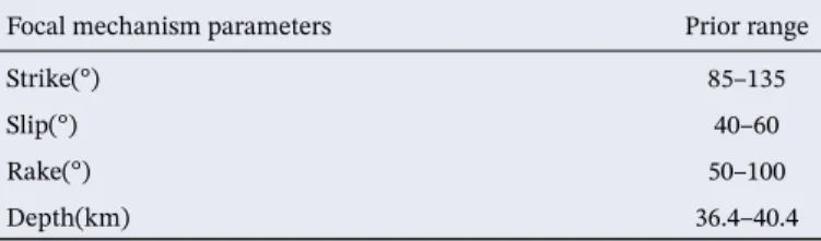
mecha-nism parameters and the source depth vary using prior uniform distributions with ranges roughly matching the MQS error estimates. The source latitude, longitude and origin time were kept fixed due to the strong trade-offs between source location and travel time. The magnitude was also kept constant and equal to the MQS estimate. The amplitude mismatch between the MSS blind test data and the predicted waveforms were corrected by energy equalization rather than including source magnitude simultaneously in the MCMC sampling, as the latter may result in the instability of the MCMC algorithm as explained in Xu and Beghe-in (2019). Details about the source priors are given in Table 2.
Figures 3 and 4 compare results of inversions performed using fixed source parameters and inversions in which the focal mechanism and focal depth were allowed to vary as explained above. Waveform envelopes were used as constraints to avoid cycle skipping. The fixed source values employed were the mean values shown in Table 2. The reference model used for both tests was the modified model of Zheng et al. (2015) as previously described and is represented by the dashed gray line. The color scale in Figure 3 represents the likelihood of a given VS model parameter. Because the model used to generate the blind test data contained a
3-D crustal model, there is a range of VS values and Moho depths along the source-receiver great circle path
Figure 2. Comparison of the MSS blind test waveform (a) and synthetic waveforms predicted by three different reference models: (b) model LVZ by Zheng et al. (2015), which included a low velocity zone; (c) model noLVZ by Zheng et al. (2015) without Low Velocity Zone; (d) Sohl and Spohn (1997)’s model A. All traces were bandpass-filtered between 25 and 50s. LVZ, low velocity zone; MSS, Mars Structure Service.
(a)
(b)
(c)
(d)
Event parameters Computed origin True origin
Origin time(UTC) January 3, 2019 15:00:53.0 January 3, 2019 15:00:30.0
Lat(°) 26.0 S 26.443 S
Lon(°) 53.0 E 50.920 E
Depth(km) 38.4 38.4
Magnitude MsM = 3.7 (Mw = 4.2) Mw = 4.46
Abbreviation: MQS, Mars Quake Service. Table 1
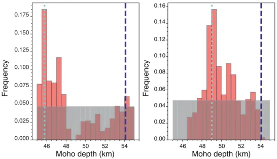
in addition to the base 1-D model that is shown in red. This range is rep-resented by the shaded area. Figure 4 shows that both the free-source test and fixed-source test favor a shallower Moho than the true value in the 1-D base model. The fixed-source test also shows a bi-modal distribution for the Moho depth, with the highest peak at about 46 km. This bi-mod-al pattern does not exist in the free-source test, which likely reflects the existence of trade-offs between source parameters, Moho depth, and Vs.
Figure 5 shows how the misfits change with the iteration number in both tests. On average, the two ensembles of models have similar misfits. Sta-tistical F-tests (Bevington et al., 1993) were performed on a number of “best” models selected in each ensemble to determine to which level of confidence the difference between model misfits is significant. They re-vealed that the two sets of inversions explain the data equivalently well. We would like to point out, however, that although the free-source inversion results do not necessarily fit the data better than to the fixed-source inversion, the former is still preferred to avoid mapping errors in the source into the velocity models since the source parameters were determined by a single station.
Figure 6 represents the source parameter posterior distributions obtained in the free source inversion in comparison to the true values used to generate the MSS blind data. Since the source is a double couple, the two complimentary planes calculated from the true source moment tensor are also plotted for comparison. We found that our posterior distribution for the strike includes and peaks near one of the two solutions cal-culated from the true source. Both possible values for the true dip are, however, outside the search range es-timated based on the MQS results. The posteriors for the slip and focal depth both show a relatively uniform
Focal mechanism parameters Prior range
Strike(°) 85–135
Slip(°) 40–60
Rake(°) 50–100
Depth(km) 36.4–40.4
Abbreviation: rj-MCMC, Monte Carlo Markov Chains. Table 2
Prior (Uniform) Distributions of Source Parameters Used for the rj-MCMC Sampling
Figure 3. Inversion results with fixed source parameters (left) and free source parameters (right). The gray dashed line represents the reference model used for MCMC sampling and partial derivative calculations. The red line is the 1-D base model used to compute the blind test data. The gray shaded area is for the maximum and minimum VS and Moho depth along the source-receiver path based on the 3-D crust model used to generate the blind test data. The color scale represents the likelihood of a given model parameter. MCMC, Monte Carlo Markov Chains.
pattern, which include but do not prefer the true values. But the posterior distribution of the strike fits well if we regard plane 2 as the true plane. The reader should be reminded that our method should, of course, not be considered as a way to jointly constrain the source parameters as well as the Martian structure. The source parameters were included to reduce the mapping of errors in the quake focal mechanism and depth into the velocity models.
3.3. Effects of Reference Crustal Thickness
The Moho depth in a Martian model can have significant influence on the synthetic waveforms, so we al-lowed it to vary in ± 5 km relative to the reference model using a linearized perturbation method as shown in Equation 2. However, this search range was still too limited to cover a wide enough set of possible Moho
Figure 4. Posterior distributions of Moho depth in the fixed-source test (left) and in the free-source test (right). The dark blue dashed lines represent the Moho depth in the 1-D base model used to generate the MSS blind test data. The light blue dotted line represents one of the best fitting values. MSS, Mars Structure Service.
Figure 5. Waveform fitting misfits as a function of iteration number for free source MCMC sampling (top) versus fixed source MCMC sampling (bottom). MCMC, Monte Carlo Markov Chains.
depths due to our yet poor prior knowledge of Martian interior. Consequently, we ran our inversions mul-tiple times, using different reference models with different Moho depths. To generate these new reference models, we changed the crustal thickness of the Zheng et al. (2015) model and proceeded as explained in Section 3.1.1: we adjusted the reference VS in order to roughly match the synthetics with the observed blind
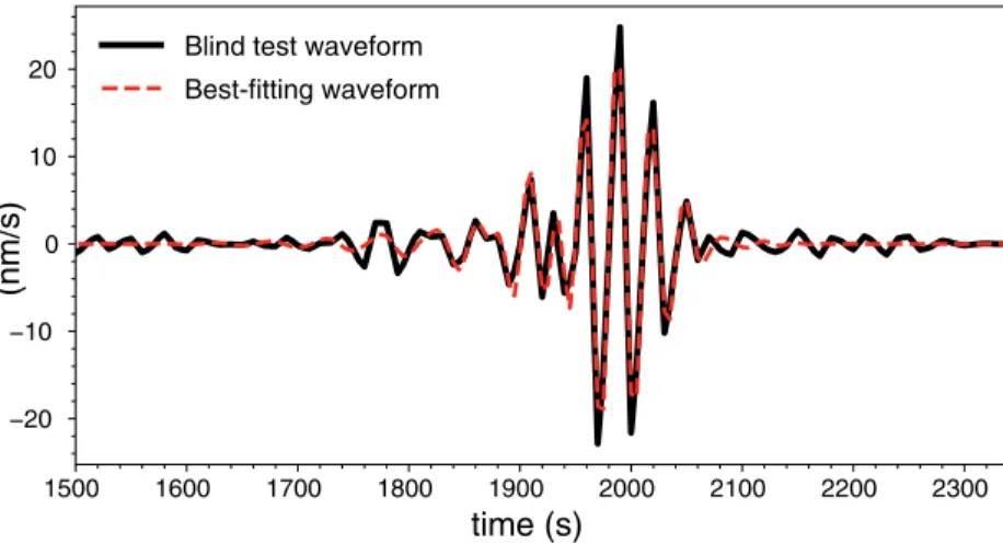
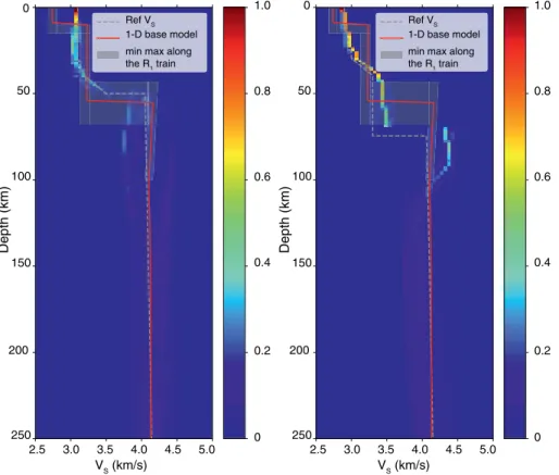
test surface waves. In Figure 7, we compare the results for model space searches done with a 50 km and a 75 km reference Moho depth. Note that while the 50 km reference Moho falls within the range of Moho depths along the source-receiver path that were used to calculate the blind test seismograms, the reference model with a 75 km Moho depth is outside of that range. Here, waveform envelopes were used as con-straints to avoid cycle skipping.
An example of best fitting waveforms is shown in Figure 8. We found that, on average, the inversions with a reference Moho depth at 50 km have a slightly lower misfit than the one with the Moho depth at 75 km. This may seem promising since the range of true Moho depth along the path did include 50 km and not 75 km depth. However, the difference in misfits did not appear to be significant and we could not simply exclude the second inversion due to its slightly higher misfit values. This is to be expected as fundamental
Figure 6. Posterior distributions of strike, dip, slip, and focal depth (red shaded area) for the inversion with free source parameters shown in the right panel of Figure 3. The prior distributions used for each of those parameters are represented by the shaded gray areas. The true values used to generate the MSS blind test data are shown by the dark blue dashed lines, including the strike, dip and slip for both planes calculated from the true source moment tensor. The best fitting parameters obtained by the MCMC sampling are indicated by the dotted line. MCMC, Monte Carlo Markov Chains; MSS, Mars Structure Service.
mode surface waves alone cannot uniquely constrain both Moho depth and velocity due to the existence of trade-offs. By comparing the VS posterior distribution to the true values used to generate the blind data, we
found that the inversions with reference Moho depth at 50 km recover the true 1-D base model better. Not only does it find posterior Moho values closer to the true values, but we also see that starting from a Moho depth that is outside of the range of true values yields a set of VS models that could be misinterpreted as
constraining a high velocity lid if care is not taken. These observations highlight how important it will be to obtain prior, independent constraints on crustal structure (e.g., from receiver functions) in order for surface waveform inversions to provide reliable velocity models.
Figure 7. Ensemble of models resulting from inversions with waveform envelopes and starting models of different crustal thickness: 50 km (left) and 75 km(right). The color scale and different curves are described in Figure 3.
3.4. Effect of Envelopes and Group Velocities
Because the envelope fit can be strongly affected by the noise level, we also tested whether the inclusion of group velocity measurements instead of the envelope affects or improves the results. The misfit function in this case is given by Equation 5. We found that the VS profiles (Figure 9)
do not strongly differ from those of Figure 7, but the range of allowable VS
models is slightly larger with the group velocities than with the envelope. Similar to Figure 7, the mean misfit was slightly lower with the reference model that has a 50 km thick crust than with the 75 km thick thrust. But, again, the difference in average misfits was not significant, so neither of these two tests can exclude one crustal thickness. By comparing the in-version results with independent group velocity measurements included versus the inversion results with waveform envelopes in the previous sec-tion, we found these two strategies yield similar VS posteriors. This is to
be expected as the envelopes of waveforms mainly provide group velocity constraints on the VS models, though group velocities may be preferable
since the envelope can be affected by noise more strongly.
We also obtained the posterior distributions of phase velocities from the ensembles of models for each test. The predictions for the four tests with free source parameters and for the true 1D base model are shown in Figure 10. Note, however, that the phase velocities calculated from the 1-D base model should not, however, be treated as the true phase velocities since the 3-D crust effects on surface wave dispersion were not taken into account. Our inverted phase velocities are lower than the phase velocities of the 1-D base model. However, for tests with
ref-Figure 9. Ensemble of models resulting from inversions with group velocities and starting models of different crustal thickness: 50 km (left) and 75 km(right). The color scale and different curves are described in Figure 3.
Figure 10. Measured phase velocity dispersion curves for the
fundamental mode Rayleigh wave with two standard deviations obtained from the posterior distributions, and dispersion curve for the 1-D base model (purple dashed curve) used in the blind test. M50 and M75 represent the inversions with Moho depth at 50 and 75 km, respectively. “Env” stands for envelope and “Grv” stands for group velocity.
3.6 3.4 3.2 3.0 2.8 25 30 35 40 45 50 1-D base model M50_Env M50_Grv M75_Env M75_Grv
erence Moho depth at 50 km, the 2σ error bars contain the 1-D base model, while for tests with reference Moho depth at 75 km, their error bars barely contain the phase velocities predicted by the 1-D base mod-el. Overall we found that the models that were obtained with a reference model whose Moho depth was included in the range of true Moho depths predict phase velocities that are closer to the 1-D base model predictions.
4. Additional Synthetic Test with Realistic Martian Noise
Since higher mode surface waves were not visible in the blind test waveforms, we created our own synthet-ic data set to test our method on a waveform with higher modes. We selected the noLVZ model of Zheng et al. (2015) to generate the synthetic waveform data due to its similarity to the MSS blind test 1-D base model. We calculated the vertical component synthetic waveforms with Mineos. Only the fundamental mode and the first three overtones were included for the purpose of this test.
In addition, we should point out that the forward modeling method used to generate the synthetic test data was the same as the forward modeling in the inversion, and a 1-D model was used to generate the synthetic data. This makes this synthetic test less challenging than the MSS blind test, for which the data were generated with a 3-D crust and a different algorithm than the one used for our forward modeling.
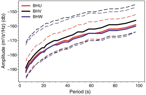
In order to generate data noise that represents a realistic overall noise level on Mars, we obtained noise amplitude information from the probabilistic power spectral density (Figure 11). The phase information for different periods were assigned randomly between [0, 2π]. Realistic Martian noise waveforms were calcu-lated by inverse Fourier Transform of the amplitude and phase information, and were superimposed to the synthetic waveforms calculated by Mineos.
One way to generate waveforms with higher mode amplitudes larger than the ambient noise is by increas-ing the magnitude of the Marsquake. However, the likelihood to have a Marsquake larger than the quake used in the blind test is not high based on the observations we have from SEIS so far. Instead, we set the magnitude of the synthetic source at the same value as for the blind test (Mw = 4.46), and tweaked other
parameters to find a scenario where the higher modes waveform is clear in the time domain and separates well from the fundamental mode. With these considerations in mind, we chose a focal depth of 40 km and an epicentral distance of 50°.
Figure 11. Probabilistic power spectral density (PPSD) measured during the “quiet” time (less windy) on Mars (18:00–23:00 LMST) in July 2019. The dashed lines mark the 10th and 90th percentiles. The PPSD was calculated using the method of McNamara and Buland (2004).
The filtered synthetic data is shown in Figure 12. It was bandpassed in the 25–50 s period range and higher modes wave trains are visible between 650 and 850 s, although the signal-to-noise ratio is on the low side. The goal of this synthetic test is to see whether our method can still resolve the higher modes and use them to constrain structure under a relatively realistic best-case scenario on Mars.
4.1. Results and Reliability Analysis
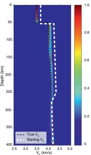
The procedures to invert this synthetic waveform is the same as for the blind test as described in detail in the previous section. The reference model was created by randomly perturbing the true model at a few depth nodes. We used waveform envelopes to avoid cycle skipping issues. Moho depth and source parameters were allowed to vary together with the ve-locity profile and the posterior noise level. The posterior VS distribution
is shown in Figure 13. We found that we can recover the true model well at most depths down to 400 km. The Markov Chains clearly converged toward the true model. We also noted that the posterior model distribution is narrower than for the blind test, likely due to the fact that the blind data set was generated with a 3-D model and ours was obtained with a 1-D model instead.
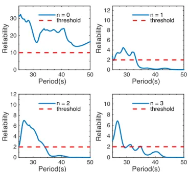
The posterior distribution of phase velocities for the multimode surface waves can be calculated using the posterior distribution of models. In theory, one can calculate an infinite number of modes from these mod-els. However, in practice, not all of them will be resolved as higher modes tend to have weaker energies and low SNR in addition to overlapping in the time domain. A reliability analysis was thus performed to determine in which modes and at which periods the phase velocities were reliably measured with our technique. In practice, for each mode, we would only keep the measurements at periods with reliability scores higher than a defined threshold. Our reliability test considers the waveform fit and the intensities of each single mode in the time-frequency domain. Further details on this reliability analysis can be found in Xu and Beghein (2019) The results of our reliability analysis for the fundamental mode and the first three overtones are given in Figure 14. We found that the fundamen-tal mode is reliably measured at all periods considered, which is identical to what is found for Earth since they have larger SNR and separate well from the higher modes. We also found, similar to Earth, that the higher modes are reliably measured at the shortest periods (<35 s in this case). Considering the sensitivity kernels for these first few higher modes (Fig-ure 1), this means that the data employed are sensitive to structure down to 300–400 km depth.In Figure 15, we plotted the dispersion curves for the reliably measured modes in addition to the dispersion curves predict-ed by the true model. The measurements are displaypredict-ed with two stand-ard deviations. We found that in all cases, the dispersion values for the true model are included within the 2σ uncertainties estimated with our method.
In Figure 16, we showed the posterior distributions of the source param-eters and Moho depth. Even though the initial model is relatively close to the true model, especially in terms of the Moho depth, we cannot re-liably use the posterior distributions of the source parameters as direct estimations of the true source. We interpret this as the outcome of strong source-structure trade-offs in this inversion problem.
Figure 12. Vertical component waveform calculated using Zheng et al. (2015)’s model noLVZ and filtered at 25–50 s (thin red line). Realistic Martian noise was added to the synthetic waveform (thick black line).
Figure 13. Ensemble of VS solutions obtained from the MCMC sampling. The thin black dashed line represents the true model and the thick white line is for the starting model. The color scale represents the likelihood of a given model parameter. MCMC, Monte Carlo Markov Chains.
Before concluding, we should remind the reader that our results do strongly depend on having a good reference model. Further analysis of the resolvability of Mars structure with higher modes under different conditions will be performed in a later study.
5. Conclusions
In this study, we presented a method to invert multimode surface-wave waveforms and measure dispersion curves based on a single station-event pair. While surface waves have not yet been observed with InSight, this method and the modifications we brought to the original technique will be important for all future seismological exploration of other planetary bodies. We showed the feasibility of our method using the MSS blind data set in the first example, and our own synthetic data in a second ex-ample. We modified our original algorithm to help account for the large uncertainties in the source parameters as well as the lack of a good Mar-tian reference model. Source parameters were included in the inversion together with the parameters describing the velocity profile in order to reduce the risk of mapping errors in the source into the models. We also added constraints from the waveform envelope to prevent cycle skipping. We showed tests for different reference models and we also compared the use of group velocities instead of envelopes.
Because the higher modes were not visible on the blind data, only the fundamental mode Rayleigh waves were inverted. We found that includ-ing the waveform envelope or group velocities did not affect the results strongly and both are good choices to prevent cycle skipping. Neither method was able to determine which reference model led to the recovery
Figure 14. Reliability scores for the fundamental mode (n = 0) and first three overtones (n = 1, 2, or 3) as a function of periods. The horizontal red dashed lines indicate the empirical thresholds we defined for each mode. Only periods with reliability scores higher than the thresholds will be kept.
Figure 15. Measured phase velocity dispersion curves for the fundamental mode Rayleigh wave (n = 0) and the first three overtones (n = 1, 2, 3) with two standard deviations as error bars. The dispersion curves from the 1-D true model (dashed curve) were plotted for comparison.
of the input 1-D base model as strong trade-offs between Moho depth and velocity structure exist. As long as the reference model has a Moho depth that is not too far from the true value, our method could find a suite of velocity models that included the true model and could measure phase velocities such that their error bars included the predictions from the true 1-D model. However, the inversions with reference Moho depths that were off the true value yielded apparent features in the VS models that could be erroneously interpreted
if care is not taken. This highlights how essential it will be to have good prior constraints on the Moho depth before inverting the surface-wave waveforms to constrain velocity structure on Mars.
In our second example, we applied the same method to synthetic data showing higher modes in the period range 25–50 s and that included realistic Martian noise levels. The higher mode wave trains in our test wave-form visible in the time domain, but very noisy. Nevertheless, by including higher modes in the inversion we were able to recover the VS structure well down to 400 km depth at true average Martian noise level, despite
the low SNR in the synthetic waveform. We further obtained the phase velocity dispersion curves for multiple modes and implemented a reliability analysis to assess which were confidently measured. Phase velocities at periods with high reliability scores generally fit the true phase velocities well. This demonstrates the feasibility of our method on higher modes measurements, though we want to stress the importance of having a good reference interior model to obtain reliable interior models with our waveform modeling approach.
Data Availability Statement
InSight seismic data presented here (http://dx.doi.org/10.18715/SEIS.INSIGHT.XB_2016) is publicly avail-able through the Planetary Data System (PDS) Geosciences node, the Incorporated Research Institutions for Seismology (IRIS) Data Management Center under network code XB and through the Data center of
Figure 16. Similar as Figure 6 but is for the synthetic test. (Red) The posterior distributions of strike, dip, slip, focal depth as well as Moho depth. The prior distributions used for each of those parameters are represented by the shaded gray areas. The true values used to generate the synthetic waveform are shown by the blue dashed lines.
Institut de Physique du Globe, Paris (http://seis-insight.eu). AH was funded by the UK Space Agency. This InSight Contribution Number 118. We acknowledge NASA, CNES, their partner agencies and Institutions (UKSA, SSO, DLR, JPL, IPGP-CNRS, ETHZ, IC, MPS-MPG) and the flight operations team at JPL, SISMOC, MSDS, IRIS-DMC and PDS for providing SEED SEIS data.
References
Anderson, O. L., Schreiber, E., Lieberman, R. C., & Soga, M. (1968). Some elastic constant data on minerals relevant to geophysics. Reviews of Geophysics, 6(4), 491–524.
Banerdt, W. B., Smrekar, S. E., Banfield, D., Giardini, D., Golombek, M., Johnson, C. L., et al. (2020). Initial results from the InSight mission on Mars. Nature Geoscience, 13, 183–189. https://doi.org/10.1038/s41561-020-0544-y
Beghein, C. (2010). Radial anisotropy and prior petrological constraints: A comparative study. Journal of Geophysical Research, 115, B03303. https://doi.org/10.1029/2008jb005842
Beghein, C., & Trampert, J. (2006). Radial anisotropy in seismic reference models of the mantle. Journal of Geophysical Research, 111, B02303. https://doi.org/10.1029/2005jb003728
Beucler, E., Stutzmann, E., & Montagner, J.-P. (2003). Surface wave higher-mode phase velocity measurements using a roller-coaster-type algorithm. Geophysical Journal International, 155(1), 289–307.
Bevington, P. R., Robinson, D. K., Blair, J. M., Mallinckrodt, A. J., & McKay, S. (1993). Data reduction and error analysis for the physical sciences. Computers in Physics, 7(4), 415–416.
Bodin, T., & Sambridge, M. (2009). Seismic tomography with the reversible jump algorithm. Geophysical Journal International, 178(3), 1411–1436.
Bodin, T., Sambridge, M., Tkalčić, H., Arroucau, P., & Gallagher, K. (2012). Transdimensional inversion of receiver functions and surface wave dispersion. Journal of Geophysical Research, 117(B2). http://dx.doi.org/10.1029/2011jb008560
Böse, M., Clinton, J., Ceylan, S., Euchner, F., Driel, M. v., Khan, A., et al. (2017). A probabilistic framework for single-station location of seismicity on Earth and Mars. Physics of the Earth and Planetary Interiors, 262, 48–65. https://doi.org/10.1016/j.pepi.2016.11.003
Cara, M. (1978). Regional variations of higher Rayleigh-mode phase velocities: A spatial-filtering method. Geophysical Journal Interna-tional, 54(2), 439–460.
Cara, M., & Lévêque, J. (1987). Waveform inversion using secondary observables. Geophysical Research Letters, 14(10), 1046–1049. Dahlen, F. (1968). The normal modes of a rotating, elliptical Earth. Geophysical Journal of the Royal Astronomical Society, 16(4), 329–367.
https://doi.org/10.1111/j.1365-246x.1968.tb00229.x
Drilleau, M., Beucler, E., Lognonné, P., Panning, M., Knapmeyer-Endrun, Banerdt, W., et al. (2020). Mss/1: Single-station and sin-gle-event marsquake inversion. Journal of Geophysical Research: Earth and Space Science. 7(12), e2020EA001118. https://doi. org/10.1029/2020EA001118
Dziewonski, A. M., Chou, T.-A., & Woodhouse, J. H. (1981). Determination of earthquake source parameters from waveform data for studies of global and regional seismicity. Journal of Geophysical Research, 86(B4), 2825–2852. https://doi.org/10.1029/JB086iB04p02825
Ekström, G., Nettles, M., & Dziewoński, A. M. (2012). The global CMT project 2004–2010: Centroid-moment tensors for 13,017 earth-quakes. Physics of the Earth and Planetary Interiors, 200–201, 1–9. https://doi.org/10.1016/j.pepi.2012.04.002
Giardini, D., Lognonné, P., Banerdt, W. B., Pike, W. T., Christensen, U., Ceylan, S., et al. (2020). The seismicity of Mars. Nature Geoscience, 13(3), 205–212. https://doi.org/10.1038/s41561-020-0539-8
Gudkova, T., & Zharkov, V. (2004). Mars: Interior structure and excitation of free oscillations. Physics of the Earth and Planetary Interiors, 142, 1–22. https://doi.org/10.1016/j.pepi.2003.10.004
Lebedev, S., & Nolet, G. (2003). Upper mantle beneath Southeast Asia from S velocity tomography. Journal of Geophysical Research, 108(B1). https://doi.org/10.1029/2000jb000073
Li, X.-D., & Romanowicz, B. (1995). Comparison of global waveform inversions with and without considering cross-branch modal cou-pling. Geophysical Journal International, 121(3), 695–709.
Li, X.-D., & Romanowicz, B. (1996). Global mantle shear velocity model developed using nonlinear asymptotic coupling theory. Journal of Geophysical Research, 101(B10), 22245–22272.
Lognonné, P., Banerdt, W. B., Giardini, D., Pike, W. T., Christensen, U., Laudet, P., et al. (2019). SEIS: Insight’s seismic experiment for internal structure of Mars. Space Science Reviews, 215(1). https://doi.org/10.1007/s11214-018-0574-6
Lognonné, P., Banerdt, W., Pike, W., Giardini, D., Christensen, U., Garcia, R., et al. (2020). Constraints on the shallow elastic and anelastic structure of Mars from InSight seismic data. Nature Geoscience. 13(3), 213–220. https://doi.org/10.1038/s41561-020-0536-y
Malinverno, A. (2002). Parsimonious Bayesian Markov Chain Monte Carlo inversion in a nonlinear geophysical problem. Geophysical Journal of the Royal Astronomical Society, 151(3), 675–688. https://doi.org/10.1046/j.1365-246x.2002.01847.x
Masters, G., Woodhouse, J., & Freeman, G. (2011). Mineos v1.0.2. [software]. Retrieved from https://geodynamics.org/cig/software/mineos/
McNamara, D. E., & Buland, R. P. (2004). Ambient noise levels in the continental United States. Bulletin of the Seismological Society of America, 94(4), 1517–1527. https://doi.org/10.1785/012003001
Meier, U., Trampert, J., & Curtis, A. (2009). Global variations of temperature and water content in the mantle transition zone from higher mode surface waves. Earth and Planetary Science Letters, 282(1–4), 91–101. https://doi.org/10.1016/j.epsl.2009.03.004
Montagner, J.-P., & Jobert, N. (1988). Vectorial tomography ii. Application to the Indian Ocean. Geophysical Journal of the Royal Astronom-ical Society, 94(2), 309–344. https://doi.org/10.1111/j.1365-246x.1988.tb05904.x
Montagner, J.-P., & Nataf, H. (1986). A simple method for inverting the Azimuthal anisotropy of surface-waves. Journal of Geophysical Research, 91(B1), 511–520. https://doi.org/10.1029/jb091ib01p00511
Nimmo, F., & Faul, U. H. (2013). Dissipation at tidal and seismic frequencies in a melt-free, anhydrous Mars. Journal of Geophysical Re-search: Planets, 118, 2558–2569. https://doi.org/10.1002/2013JE004499
Nolet, G. (1975). Higher Rayleigh modes in western Europe. Geophysical Research Letters, 2(2), 60–62.
Nolet, G. (1990). Partitioned waveform inversion and two-dimensional structure under the network of autonomously recording seismo-graphs. Journal of Geophysical Research, 95(B6), 8499–8512.
Panning, M., Beucler, É., Drilleau, M., Mocquet, A., Lognonné, P., & Banerdt, W. B. (2015). Verifying single-station seismic approaches using earth-based data: Preparation for data return from the insight mission to Mars. Icarus, 248, 230–242.
Acknowledgments
C. Beghein and H. Xu were funded for this research by NASA InSight PSP grant #80NSSC18K1679. M.P.P. was supported by the NASA InSight mission and funds from the Jet Propulsion Lab-oratory, California Institute of Technol-ogy, under a contract with the National Aeronautics and Space Administration (80NM0018D0004).
Panning, M., Lognonné, P., Banerdt, W. B., Garcia, R., Golombek, M. P., Kedar, S., et al. (2017). Planned products of the Mars structure Service for the InSight mission to Mars. Space Science Reviews, 211, 611–650. https://doi.org/10.1007/s11214-016-0317-5
Panning, M., & Romanowicz, B. (2006). A three-dimensional radially anisotropic model of shear velocity in the whole mantle. Geophysical Journal of the Royal Astronomical Society, 167(1), 361–379. https://doi.org/10.1111/j.1365-246x.2006.03100.x
Smrekar, S. E., Lognonné, P., Spohn, T., Banerdt, W. B., Breuer, D., Christensen, U., et al. (2019). Pre-mission InSights on the interior of Mars. Space Science Reviews, 215(1), 3. https://doi.org/10.1007/s11214-018-0563-9
Sohl, F., & Spohn, T. (1997). The interior structure of Mars: Implications from SNC meteorites. Journal of Geophysical Research, 102, 1613–1635. https://doi.org/10.1029/96JE03419
Stähler, S. C., & Sigloch, K. (2016). Fully probabilistic seismic source inversion-part 2: Modelling errors and station covariances. Solid Earth, 7(6), 1521–1536.
Valentine, A., & Woodhouse, J. (2010). Reducing errors in seismic tomography: Combined inversion for sources and structure. Geophysical Journal of the Royal Astronomical Society, 180(2), 847–857. https://doi.org/10.1111/j.1365-246x.2009.04452.x
van Driel, M., Ceylan, S., Clinton, J. F., Giardini, D., Alemany, H., Allam, A., et al. (2019). Preparing for InSight: Evaluation of the blind test for Martian seismicity. Seismological Research Letters, 90(4), 1518–1534. https://doi.org/10.1785/0220180379
van Heijst, H. J., & Woodhouse, J. (1997). Measuring surface-wave overtone phase velocities using a mode-branch stripping technique. Geophysical Journal International, 131(2), 209–230.
van Heijst, H. J., & Woodhouse, J. (1999). Global high-resolution phase velocity distributions of overtone and fundamental-mode surface waves determined by mode branch stripping. Geophysical Journal International, 137(3), 601–620.
Visser, K. (2008). Monte Carlo search techniques applied to the measurement of higher mode phase velocities and anisotropic surface wave tomography. Geologica Ultraiectina (285). Utrecht, The Netherlands: Departement Aardwetenschappen. (OCLC: 6893359236). Retrieved from http://dspace.library.uu.nl/handle/1874/26448
Visser, K., Lebedev, S., Trampert, J., & Kennett, B. (2007). Global Love wave overtone measurements. Geophysical Research Letters, 34(3).
https://doi.org/10.1029/2006gl028671
Woodhouse, J. (1980). The coupling and attenuation of nearly resonant multiplets in the earth’s free oscillation spectrum. Geophysical Journal of the Royal Astronomical Society, 61(2), 261–283. https://doi.org/10.1111/j.1365-246x.1980.tb04317.x
Xu, H., & Beghein, C. (2019). Measuring higher mode surface wave dispersion using a transdimensional Bayesian approach. Geophysical Journal International, 218(1), 333–353. https://doi.org/10.1093/gji/ggz133
Yoshizawa, K., & Ekström, G. (2010). Automated multimode phase speed measurements for high-resolution regional-scale tomography: Application to North America. Geophysical Journal International, 183(3), 1538–1558.
Yoshizawa, K., & Kennett, B. (2002). Non-linear waveform inversion for surface waves with a neighbourhood algorithm—Application to multimode dispersion measurements. Geophysical Journal International, 149(1), 118–133.
Zheng, Y., Nimmo, F., & Lay, T. (2015). Seismological implications of a lithospheric low seismic velocity zone in Mars. Physics of the Earth and Planetary Interiors, 240, 132–141. https://doi.org/10.1016/j.pepi.2014.10.004