HAL Id: hal-00317603
https://hal.archives-ouvertes.fr/hal-00317603
Submitted on 30 Mar 2005
HAL is a multi-disciplinary open access
archive for the deposit and dissemination of
sci-entific research documents, whether they are
pub-lished or not. The documents may come from
teaching and research institutions in France or
abroad, or from public or private research centers.
L’archive ouverte pluridisciplinaire HAL, est
destinée au dépôt et à la diffusion de documents
scientifiques de niveau recherche, publiés ou non,
émanant des établissements d’enseignement et de
recherche français ou étrangers, des laboratoires
publics ou privés.
The effects of the pre-reversal ExB drift, the EIA
asymmetry, and magnetic activity on the equatorial
spread F during solar maximum
C.-C. Lee, J.-Y. Liu, B. W. Reinisch, W.-S. Chen, F.-D. Chu
To cite this version:
C.-C. Lee, J.-Y. Liu, B. W. Reinisch, W.-S. Chen, F.-D. Chu. The effects of the pre-reversal ExB
drift, the EIA asymmetry, and magnetic activity on the equatorial spread F during solar maximum.
Annales Geophysicae, European Geosciences Union, 2005, 23 (3), pp.745-751. �hal-00317603�
© European Geosciences Union 2005
Geophysicae
The effects of the pre-reversal drift, the EIA asymmetry, and
magnetic activity on the equatorial spread F during solar maximum
C.-C. Lee1, J.-Y. Liu2, B. W. Reinisch3, W.-S. Chen2, and F.-D. Chu2,4
1General Education Center, Ching-Yun University, No. 229, Chienshin Road, Jhongli City, Taoyuan County 320, Taiwan 2Institute of Space Science, National Central University, No. 300, Jhongda Rd., Jhongli City, Taoyuan County 320, Taiwan 3Center for Atmospheric Research, University of Massachusetts Lowell, 600 Suffolk Street, Lowell, MA 01854, USA 4National Standard Time and Frequency Laboratory, Telecommunication Laboratories, No. 12 Lane 551 Ming-Tsu Road
Sec. 5, Yang-Mei 326, Taiwan
Received: 23 July 2004 – Revised: 15 December 2004 – Accepted: 10 January 2005 – Published: 30 March 2005
Abstract. We use a digisonde at Jicamarca and a chain
of GPS receivers on the west side of South America to in-vestigate the effects of the pre-reversal enhancement (PRE) in E×B drift, the asymmetry (Ia)of equatorial ionization
anomaly (EIA), and the magnetic activity (Kp) on the
gener-ation of equatorial spread F (ESF). Results show that the ESF appears frequently in summer (November, December, Jan-uary, and February) and equinoctial (March, April, Septem-ber, and October) months, but rarely in winter (May, June, July, and August) months. The seasonal variation in the ESF is associated with those in the PRE E×B drift and Ia.
The larger E×B drift (>20 m/s) and smaller |Ia|(<0.3) in
summer and equinoctial months provide a preferable condi-tion to development the ESF. Conversely, the smaller E×B drift and larger |Ia| are responsible for the lower ESF
oc-currence in winter months. Regarding the effects of mag-netic activity, the ESF occurrence decreases with increasing Kpin the equinoctial and winter months, but not in the
sum-mer months. Furthermore, the larger and smaller E×B drifts are presented under the quiet (Kp<3) and disturbed (Kp≥3)
conditions, respectively. These results indicate that the sup-pression in ESF and the decrease in E×B drifts are mainly caused by the decrease in the eastward electric field.
Keywords. Ionosphere (ionospheric irregularities;
equato-rial ionosphere)
1 Introduction
Equatorial spread F (ESF) takes its name from the range-dispersed ionogram at stations near the dip equator (Booker and Well, 1938). The ESF usually occurs just after local sun-set and the scale sizes of irregularities range from a few cen-timeters to a few hundred kilometers. Based on the previ-ous investigations, the basic mechanism of ESF onset is the gravitational Rayleigh-Taylor (GRT) instability in
conjunc-Correspondence to: C.-C. Lee
tion with the E×B drift instability (e.g. Kelley, 1989; Abdu, 2001). The growth rate of instabilities crucially depends on the density gradient that becomes steeper in the nighttime equatorial F-region. Moreover, due to the nonlinear evolu-tion, these instabilities would fully develop into vertically elongated wedges of plasma depletion from bottomside to topside of the F-layer (e.g. Tsunoda et al., 1982; Zalesack et al., 1982; Sultan, 1996).
The ESF studies using ionosonde data (Sales et al., 1996; Stephan et al., 2002; Whalen, 2002), the Global Positioning System (GPS) (Aarons et al., 1996; Mendillo et al., 2000, 2001), radars (Woodman and LaHoz, 1976; Hysell and Bur-cham, 1998), satellite (Huang et al., 2001; Su et al., 2001), and numerical modeling (Maruyama, 1988; Sultan, 1996) have demonstrated the general morphology of the ESF phe-nomenon. Now, it is known that there are some candidate mechanisms helping the ESF development. These are (1) the pre-reversal enhancement (PRE) in upward E×B drift and associated uplifting of the F-layer (Fejer et al., 1999; Whalen, 2002), (2) a small or null transequatorial compo-nent of the thermospheric winds and associated symmetry in the equatorial ionization anomaly (EIA) (Maruyama and Matuura, 1984; Maruyama, 1988; Mendillo et al., 2000, 2001), (3) a simultaneous decay of the E region conductiv-ity at both ends of the field line (Tsunoda, 1985; Stephan et al., 2002), and (4) a sharp gradient at the bottomside of the F-layer (Kelley, 1989).
The scope of this paper is to look for the effects of the first and second mechanisms listed above on the ESF onset. For two decades, the earlier works have investigated the variabil-ity of E×B drift on various timescales from day-to-day to season, on longitude, and on solar and geomagnetic activi-ties. Fejer et al. (1979) examined the vertical drift measure-ments of Jicamarca (12◦S, 76.9◦W) incoherent scatter radar (ISR) during 1968–1976 to find the associated variations in season and solar cycle. Abdu et al. (1983) pointed out that a necessary condition for the ESF occurrence is the E×B drift from analysis of Fortaleza (4◦S, 38◦W) ionosonde data during January–April and September–December in 1978.
746 C. C. Lee et al.: The equatorial spread F during solar maximum
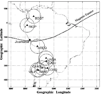
Table 1. The locations of the GPS stations on the west side of South America.
GPS Station Geographical Latitude Geographical Longitude Geomagnetic Latitude
Bogota (BOGT) 4.6◦N 74.1◦W 16.7◦N
Riobamba Permanent Station (RIOP) 1.6◦S 78.6◦W 10.4◦N Arequipa Laser Station (AREQ) 16.5◦S 71.5◦W 3.2◦S UNSA Salta (UNSA) 24.7◦S 65.4◦W 12.2◦S
Tucuman (TUCU) 26.8◦S 65.2◦W 14.3◦S
Coronel Fontana (CFAG) 31.6◦S 68.2◦W 18.4◦S
Cordoba (CORD) 31.7◦S 64.5◦W 18.9◦S
Valparaiso Tide Gauge (VALP) 33.0◦S 71.6◦W 19.6◦S Santiago Tracking Station (SANT) 33.1◦S 70.7◦W 19.7◦S
Fig. 1. Map of a digisonde and a chain of nine GPS receivers. The
solid dot represents the Jicamarca digiosonde, while the triangles symbolize the nine GPS stations on the west side of South America. The circles at each GPS site give the field-of-view for a 400-km intersection height at an elevation angle at 30◦.
Recently, Fejer et al. (1999) analyzed the data of the Jica-marca ISR during 1968–1992, and found that the E×B drift and ESF occurrence depend on solar flux, season, and mag-netic activity. Whalen (2002) also proposed that the ESF oc-currence and E×B drift are a function of magnetic activity and season, using an array of ionospheric sounders in the western American sector during 1958.
Among the studies made on the effects of the second mechanism, most studies employed the short-duration data to explore the day-to-day variability of the meridional wind and associated EIA asymmetry. Maruyama and Matuura (1984) proposed that the asymmetry in the electron density distri-bution, which is caused by the meridional winds, could sup-press the ESF activity. However, they did not show the sea-sonal variation in the asymmetry in the density distribution.
Fig. 2. Sample for h0F (bold line) and dh0F/dt (thin line) on 15 April 1999. The maximum value of dh0F/dt is ∼32 m/s.
Furthermore, Mendillo et al. (1992) have noted the possi-ble contributions of transequatorial wind in limited samples of ESF day-to-day variability, using an all-sky imaging sys-tem at Kwajalen Atoll (9.4◦N, 167.5◦E). Sastri et al. (1997) applied two ionosondes in Brazil to examine the correlation between the ESF occurrences and the associated meridional winds in June of 1978–1981. Mendillo et al. (2000, 2001) utilized the GPS data near the equinox to calculate the asym-metry of EIA and to test the day-to-day variability of ESF.
In the present paper, we first attempt to investigate the sea-sonal effect of the EIA asymmetry on the ESF development, besides the seasonal effect of the PRE E×B drift velocity and the magnetic activity. We conducted a one-year observa-tion on the equatorial ionosphere during April 1999–March 2000. A digisonde and a chain of GPS receivers on the west side of South America have been applied to this work. The minimum virtual height of the F-layer (h0F) and the latitudi-nal distribution of the vertical total electron content (VTEC) are used to derive the PRE E×B drift and the asymmetry of EIA, respectively. Further, we utilize these data to study the dependence of ESF on the PRE E×B drift velocity, the asymmetry of EIA, and the magnetic activity (Kp).
Fig. 3. Schematic illustrating a typical latitudinal distribution of
VTEC values. The equation of an asymmetry index Iaof the EIA
is represented in the upper-right corner.
2 Experiment setup
Figure 1 shows the locations of a digisonde and all nine GPS receivers. The Jicamarca digisonde (12◦S, 76.9◦W, geomagnetic latitude: 1.28◦N), near the geomagnetic equa-tor, recorded ionograms from April 1999 to March 2000. The presence/absence of ESF and the ionospheric parameters (e.g. h0F, foF2 – maximum frequency of F-layer) are
deter-mined by both the ARTIST program (Reinisch and Haung, 1983; Reinisch, 1996) and manual work. Notably, we focus on the ESF appearing during 18:00–24:00 LT (LT=UT–5 h). The upward PRE velocity is derived by the temporal rate of of h0F, dh0F/dt, which is described as the E×B drift veloc-ity (Bittencourt and Abdu, 1981). Since the E×B velocveloc-ity generally reaches its maximum value before the onset of ESF (e.g. Fejer et al., 1999; Whalen, 2002), we apply the maxi-mum value of dh0F/dt between 18:00 LT and the time of ESF onset to the statistical analyses. For example (Fig. 2), as the ESF appears from 19:15 LT on 15 April 1999, the maximum value of dh0F/dt, ∼32 m/s, is adopted in the following stud-ies.
The data of the nine GPS sites (Fig. 1 and Table 1) are retrieved from the International GPS Service (IGS) for Geo-dynamics. Two of the GPS sites (BOGT and RIOP) are situ-ated north of the geomagnetic equator, and the BOGT site is located near the northern crest of EIA. The other seven GPS receivers (AREQ, UNSA, TUCU, CFAG, CORD, VALP, and SANT) are placed south of the equator. The AREQ is close to the equator, while the TUCU is located near the south-ern crest. These nine GPS sites offer the equivalent VTEC along the common meridian of ∼75◦W (see Mendillo et al., 2000 for reference). Moreover, an asymmetry index of EIA (Ia), which is related to the transequatorial meridional
winds, can be derived from the north versus south crest dif-ferences. The Ia is represented as (N–S)/((N+S)/2) (shown
in Fig. 3), where N and S are the VTEC values of the north and south crests, respectively (Mendillo et al., 2000). Based on Abdu (2001), the ESF development would depend upon
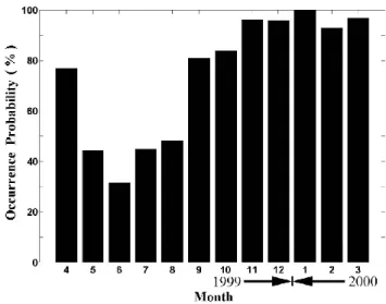
Fig. 4. Seasonal variation in the occurrence probability of ESF
during April 1999–March 2000. The highest value (100%) of the occurrence probability appears in January, while the lowest value (30%) is at June.
the symmetry/asymmetry of EIA during the previous 0.5- to 1-h period. Therefore, we examine the Iabetween 18:00 LT
and the time of ESF onset. While Iais positive/negative
dur-ing this period, the maximum/minimum value of Iais used
for the statistical analyses. Notably, Iais not estimated
dur-ing December 1999–March 2000, because the BOGT data are not available in these months.
3 Results and discussion
3.1 Seasonal variations in occurrence probability of ESF Figure 4 displays the seasonal variation in the occurrence probability of ESF. This seasonal variation in the occurrence probability is the percentage of days on which at least one pre-midnight ESF event is observed daily. Clearly, the high-est occurrence probabilities (100%) of ESF is in January, near the summer solstice; while the lowest values (∼32%) is in June, near the winter solstice. During the equinoctial months (March, April, September, and October), the occur-rence probabilities are more than 75%. Generally, the oc-currence probability is higher in summer (November, De-cember, January, and February)/equinoctial months than in winter months (May, June, July, and August). In this in-vestigation, the ESF is not categorized into three levels pro-posed by Whalen (2002), because only one ionosonde is used. Thus, the seasonal variation in ESF (Fig. 4) should be compared with that in the total bottomside spread F (BSSF) of Whalen (2002) (his Fig. 4), who analyzed the ionograms at Huancayo (12◦S, 75.3◦W) during 1958. Notice that the total BSSF consists of strong and weak BSSF and bubbles (Whalen, 2002), and Huancayo is located at 160 km east of Jicamarca. The comparison result shows that these two
748 C. C. Lee et al.: The equatorial spread F during solar maximum
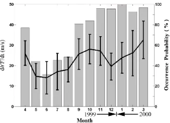
Fig. 5. Seasonal variation in the monthly mean value of the dh0F/dt (soild line) and the associated standard deviation (error bar) during April 1999–March 2000. The gray histogram in the background represents the occurrence probability of ESF. Two peak values of dh0F/dt appear at October and March, while the smallest value is at June.
seasonal variations are similar: the highest and lowest occur-rence probabilities are in summer and winter, respectively. 3.2 Seasonal variations in the PRE E×B drift
We examine the seasonal variation in the PRE E×B drift by deriving the monthly mean value of dh0F/dt. Figure 5 shows the seasonal variation in the monthly mean value of dh0F/dt (solid line) and the associated standard deviation (error bar), as well as the occurrence probability of ESF (gray histogram in background). It is apparent that two peak values, ∼28 and ∼32 m/s, appear in October and March, respectively; while the smallest dh0F/dt, ∼14 m/s, is in June. The seasonal
varia-tion in dh0F/dt is close to Fejer et al. (1999), who propounded that the largest and smallest vertical drift velocities are at the equinox and the June solstices, respectively. Consequently, the mean dh0F/dt are ∼14–18 and ∼20–27 m/s during May-August and November-February, respectively. These mean values are also close to Fejer et al. (1999), in which the max-imum values are ∼18 and ∼28–34 m/s, respectively, in May– August and November–February, during a high solar activity period. However, in March, April, September, and October, the values of ∼25–32 m/s are slightly smaller than the maxi-mum value (∼33–48 m/s) of Fejer et al. (1999) during a high solar activity period.
In the equinoctial months, the larger dh0F/dt is associated with the higher ESF occurrence. This demonstrates that the larger upward drift lifts the F-layer to higher altitudes, which not only results in favorable conditions for the GRT insta-bility but the larger eastward electric field itself causes an E×B drift instability (Maruyama, 1988; Kelley, 1989). In contrast, the small dh0F/dt in the winter months would not raise the F-layer to altitudes where it is high enough to gener-ate irregularities. Thus, the ESF occurrences are lower in the
Fig. 6. Seasonal variation in the monthly mean value of Ia (soild
line) and the associated standard deviation (error bar) during April 1999-March 2000. The gray histogram in the background repre-sents the occurrence probability of ESF. Notice that Iais not
esti-mated during December 1999–March 2000, because the GPS data of BOGT are not available in these months.
winter months. These results reveal that the PRE E×B drift plays an important role as the seeding mechanism of ESF development (Sultan, 1996; Fejer et al., 1999; Kudeki and Bhattacharyya, 1999; Whalen, 2002). Additionally, there are also other seeding mechanisms such as gravity waves (Sul-tan, 1996; Kudeki and Bhattacharyya, 1999).
During the summer months, the mean values of dh0F/dt, ∼20–27 m/s, are smaller than that at the equinox, but higher than that in the winter. Notice that the occurrence probability of ESF in January is the highest value (100%) between April 1999 and March 2000. Such kind of correlation between the dh0F/dt and the ESF occurrence indicates that there would be another mechanism to help the ESF development, besides the larger upward velocity. According to Maruyama (1988) and Fejer et al. (1999), the late reversal time of upward drift should be a considerable reason for the highest occurrence probability at December solstice.
3.3 Seasonal variations in the asymmetry of EIA
Figure 6 shows the seasonal variation in the monthly mean value of Ia(solid line), the associated standard deviation
(er-ror bar), and the occurrence probability of ESF (gray his-togram in background). It is found that Ia is negative and
|Ia|is greater than 0.3 during May–August (winter months).
In April, September, and October (equinoctial months), Iais
also negative, but |Ia|is smaller than 0.3. In contrast, Iais
positive and |Ia|is smaller than 0.3 in November (summer
months). According to Mendillo et al. (2000, 2001), the Ia
index is associated with the transequatorial meridional winds that would distort a presumed symmetrical EIA. Thus, the meridional winds are generally southward and northward in April-October and November, respectively. Moreover, the greater values (>0.3) of |Ia| during May-August indicate
Fig. 7. Occurrence of ESF on each day for each of the equinoctial (a), summer (b), and winter (c) months plotted as a function of Kp
determined as the average during the 6 h prior to measurement.
that the associated meridional winds in the winter months are stronger than that in the equinoctial (April, September, and October) and summer (November) months. These are similar to the meridional winds used by Maruyama (1988), in which the wind is northward and stronger near the winter solstice (in his Fig. 3).
As shown in Fig. 6, the greater |Ia| and lower ESF
oc-currence concurrently appear during May-August. Based on Maruyama and Matuura (1984), Maruyama (1988), and Mendillo et al. (1992), this negative correlation between these two parameters indicates that the asymmetric EIA is re-lated to the inhibition of ESF development. This is because the asymmetry of EIA would form an asymmetry in distribu-tion of conductivity and recombinadistribu-tion rates along the field line. Then, the asymmetry in conductivity and recombination rates further suppresses the GRT growth rate (Maruyama and Matuura, 1984; Maruyama, 1988; Mendillo et al., 1992). Be-sides the suppressive effect of Ia, the smaller dh0F/dt in the
winter months (Fig. 5) is not helpful in developing the ESF either. Therefore, the lower ESF occurrence is caused by the greater |Ia|and the smaller dh0F/dt.
On the other hand, the smaller |Ia| and higher ESF
oc-currence concurrently appear in April, September, and Octo-ber. This result shows that the |Ia|is negatively correlated
with the ESF occurrence, and demonstrates that the asym-metry in conductivity and recombination rates would be not strong enough to suppress the GRT growth rate. Recall that, in the equinoctial months (Fig. 5), the values of dh0F/dt are larger. Thus, the higher ESF occurrence is due to not only the larger dh0F/dt but also the smaller |Ia|during the equinoctial
months. Additionally, the smaller |Ia|and higher ESF
occur-rence are also seen simultaneously in November. Similar to the equinoctial months, the higher ESF occurrence is caused by both the smaller |Ia|and larger dh0F/dt.
3.4 Dependence on the magnetic activity (Kp)
The ESF is examined on each day in relation to the magnetic activity on that day, which is taken as the average value of Kp recorded during the 6 h prior to the onset of ESF (e.g.
Fejer et al., 1999; Whalen, 2002). Notice that the average Kpis generally derived from the interval of 18:00–24:00 UT
(13:00–19:00 LT).
The number of days on ESF are organized by season and plotted versus the average Kpin Fig. 7. For the equinoctial
months (Fig. 7a), the ESF occurs frequently and rarely when Kp is 1 and 5, respectively. Except Kp=2, the number of
days tends to decrease with increasing Kp in the
equinoc-tial months. Moreover, a descending trend from Kp=1 to
5 is obvious in the winter months (Fig. 7c), but not in the summer months (Fig. 7b). The decreasing trends in the equinoctial and winter months indicate that the increasing magnetic activity progressively suppresses the ESF genera-tion in these two seasons (Fejer et al., 1999; Whalen, 2002). However, these distributions are not consistent with that of total BSSF in Whalen (2002) (his Fig. 5), which reported that the decreasing trends existed in the equinoctial and summer months, not in the winter months. This might be because the distribution of Kpdays is different for each seasons between
1958 and 1999–2000.
To further reveal the geomagnetic effect on dh0F/dt and Ia, we examine the monthly mean values of dh0F/dt (Fig. 8a)
and Ia(Fig. 8b) under quiet (Kp<3) and disturbed (Kp≥3)
conditions during April 1999–March 2000. In the equinoc-tial months, the mean dh0F/dt as Kp≥3 is less than that as
Kp<3, and the differences are ∼3–8 m/s. For the summer
months, dh0F/dt is larger under the quiet condition and the differences are ∼2–5 m/s, except February. Furthermore, for the winter months, dh0F/dt as K
p<3 is also larger in May and
August, and the differences are ∼8 and ∼3 m/s, respectively. Notice that no dh0F/dt as K
p≥3 is shown in June, because
all Kpare smaller than 3. Furthermore, only one dh0F/dt as
Kp≥3 is in July, and this large upward velocity is related
to the prompt penetration effect (Fejer and Scherliess, 1997; Fejer et al., 1999). Generally, the dh0F/dt is smaller under the disturbed condition, and these results are similar to Fe-jer et al. (1999), who proposed that the maximum vertical drift is, respectively, larger and smaller under the quiet and disturbed conditions during a high solar activity period (their Fig. 7). The decrease in dh0F/dt indicates that the maximum
750 C. C. Lee et al.: The equatorial spread F during solar maximum
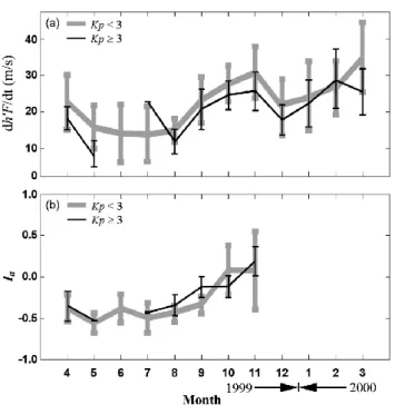
Fig. 8. Seasonal variations of the monthly mean values of dh0F/dt
(a) and Ia(b) between April 1999 and March 2000. The black thin
and gray bold lines represent the mean values under the disturbed (Kp≥3) and quiet (Kp<3) conditions, respectively. The error bars
are the associated standard deviation.
eastward electric field of PRE is reduced by the disturbed magnetic activity (Scherliess and Fejer, 1997). Moreover, this decrease is due to the disturbance dynamo electric fields which decrease the upward drift velocity near sunset (Fejer et al., 1999).
Regarding the Ia(Fig. 8b), it is found that the mean |Ia|as
Kp<3 is larger than that as Kp≥3 in August and September.
In contrast, the mean |Ia| as Kp<3 is smaller than that as
Kp≥3 in October and November. Moreover, the mean |Ia|is
nearly the same between the quiet and disturbed conditions in April, May, and July. These results suggest that the effect of the magnetic activity on Iaseems not to be evident. Since the
Iais related tothe meridional winds, the disturbed magnetic
activity does not obviously affect the strength of the winds.
4 Summary and conclusion
We have analyzed the ionogram and TEC data to investigate the long-duration effects of the PRE E×B drift, the EIA asymmetry, and the magnetic activity on the ESF generation. The ionogram and TEC data during April 1999–March 2000 are obtained by a digisonde and a chain of GPS receivers, re-spectively. It is remarkable that this work is a first attempt to examine the seasonal variation in the EIA asymmetry. The results point out that the dependence of ESF on season and magnetic activity can be explained by the corresponding ef-fects on the E×B drift and EIA asymmetry.
For the seasonal variation, the ESF appears frequently in the summer and equinoctial months, but rarely in the
winter months. Such kind of occurrence variation is evi-dently correlated to the magnitude of E×B drift. The corre-lations in summer and equinoctial months demonstrate that the ionosphere is lifted to higher altitudes where the gravita-tional drift term is dominant in the GRT growth rate, leading to the development of the ESF, when the upward drift veloc-ities are larger than 20 m/s. Moreover, the influence of the EIA asymmetry (Ia)is also significant regarding the ESF
oc-currence. The value of |Ia|is generally anti-correlated to the
ESF occurrence. This anti-correlation indicates that the EIA asymmetry (|Ia|>0.3) could suppress the GRT growth rate,
because of the asymmetry in distribution of conductivity and recombination rates.
For the magnetic activity, we have shown that the number of ESF days decreases with increasing Kp in the
equinoc-tial and winter months, but not in the summer months. This descending trend suggests that the magnetic activity progres-sively suppresses the ESF generation in those two months. Additionally, our results shows that the E×B velocity is larger and smaller under the quiet and disturbed conditions, respectively. This indicates that this ESF suppression would be due to the effect of the magnetic activity on the E×B ve-locity. Contrarily, it is found that Iais not obviously related
to the magnetic activity.
Acknowledgements. This work is supported by the grant of
Na-tional Science Council: NSC 2119-M-231-002 and NSC 93-2111-M-008-022-AP5. The authors would like to thank the Inter-national GPS Service (IGS) for Geodynamics for GPS data and to the World Data Center for Geomagnetism in Kyoto for providing
Kpdata.
Topical Editor M. Lester thanks a referee for his/her help in evaluating this paper.
References
Aarons, J., Mendillo, M., and Yantosca, R.: GPS phase fluctuations in the equatorial region during the MISETA 1994 campaign, J. Geophys. Res., 101, 26 851–26 862, 1996.
Abdu, M. A.: Outstanding problems in the equatorial ionosphere-thermosphere electrodynamics relevant to spread F, J. Atmos. Solar-Terr. Phys., 63, 869–884, 2001.
Abdu, M. A., de Medeiros, R. T., Bittencourt, J. A., and Batista, I. S.: Vertical ionization drift velocities and range type spread in the evening equatorial ionosphere, J. Geophys. Res., 88, 399– 402, 1983.
Bittencourt, J. A. and Abdu, M. A.: A theoretical comparison be-tween apparent and real verical ionization drift velocities in the equatorial F-region, J. Geophys. Res., 86, 2451–2454, 1981. Booker, H. G. and Wells, H. W.: Scattering of radio waves by the
F-region of the ionosphere, J. Geophys. Res., 43, 249–256, 1938. Fejer, B. G. and Scherliess, L.: Empirical models of storm time equatorial zonal electric fields, J. Geophys. Res., 102, 24 047– 24 056, 1997.
Fejer, B. G., Farley, D. T., Woodman, R. F., and Calderon, C.: De-pendence of equatorial F-region vertical drifts on season and so-lar cycle, J. Geophys. Res., 84, 5792–5796, 1979.
Fejer, B. G., Scherliess, L., and de Paula, E. R.: Effects of the verti-cal plasma drift velocity on the generation and evolution of equa-torial F, J. Geophys. Res., 104, 19 859–19 869, 1999.
Huang, C. Y., Burke, W. J., Machuzak, J. S., Gentile, L. C., and Sultan, P. J.: DMSP observations of equatorial plasma bubbles in the topside ionosphere near solar maximum, J. Geophys. Res., 106, 8131–8142, 2001.
Hysell, D. L. and Burcham, J. D.: JULIA radar studies of equatorial spread F, J. Geophys. Res., 103, 29 155–29 167, 1998.
Kelley, M. C.: The Earth’s Ionosphere, Int. Geophys. Ser., Aca-demic, San Diego, Calif., 43, 1989.
Kudeki, E. and Bhattacharyya, S.: Post sunset vortices in equatorial F-region plasma drifts and implications for bottomside spread F, J. Geophys. Res., 104, 28 163–28 170, 1999.
Maruyama, T.: A diagnostic model for equatorial spread F 1. model description and application to electric field and neutral wind ef-fects, J. Geophys. Res., 93, 14 611–14 622, 1988.
Maruyama, T. and Matuura, N.: Longitudinal variability of annul changes in activity of equatorial spread F and plasma depletions, J. Geophys. Res., 89, 10 903–10 912, 1984.
Mendillo, M., Baumgardner, J., Pi, X., and Sultan, P. J.: Onset conditions for equatorial spread F, J. Geophys. Res., 97, 13 865– 13 876, 1992.
Mendillo, M., Lin, B., and Aarons, J.: The application of GPS ob-servation to equatorial aeronomy, Radio Sci., 35, 885–904, 2000. Mendillo, M., Meriwether, J., and Miodni, M.: Testing the ther-mospheric neutral wind suppression mechanism for day-to-day variability of equatorial F, J. Geophys. Res., 106, 3655–3663, 2001.
Reinisch, B. W.: Modern ionosondes, in: Modern Radio Science, edited by: Kohl, H., Ruester, R., and Schlegel, K., European Geophysical Society, Katlenburg-Lindau, Germany, 440–458, 1996.
Reinisch, B. W. and Haung, X.: Automatic calculation of electron density profiles from digital ionograms, 3. Processing of bottom-side ionograms, Radio Sci., 18, 477–492, 1983.
Sales, G. S., Reinisch, B. W., Scali, J. L., Dozois, C., Bullett, T. W., Weber, E. J., and Ning, P.: Spread-F and the structure of equa-torial ionization depletions in the Southern Anomaly Region, J. Geophys. Res., 101, 26 819–26 827, 1996.
Sastri, J. H., Abdu, M. A., Batista, I. S., and Sobral, H. A.: On-set conditions of equatorial (range) spread F at Fortaleza, Brazil, during the Jun solstice, J. Geophys. Res., 102, 24 013–24 021, 1997.
Scherliess, L. and Fejer, G. B.: Storm time dependence of equatorial disturbance dynamo zonal electric fields, J. Geophys. Res., 102, 24 037–24 046, 1997.
Stephan, A. W., Colerico, M., Mendillo, M., Reinisch, B. W., and Anderson, D.: Suppression of equatorial spread F by sporadic E, J. Geophys. Res., 107 (A2), doi:10.1029/2001JA000162, 2002. Su, S. Y., Yeh, H. C., and Heelis, R. A.: ROCSAT-1 IPEI
observa-tions of equatorial spread F-some early transitional scale results, J. Geophys. Res., 106, 29 153–29 159, 2001.
Sultan, P. J.: Linear theory and modeling of the Rayleigh-Talor in-stability leading to the occurrence of equatorial F, J. Geophys. Res., 101, 26 875–26 891, 1996.
Tsunoda, R.: Control of the seasonal and longitudinal occurrence of equatorial scintillations by the longitudinal gradient in the in-tegrated E region Pedersen conductivity, J. Geophys. Res., 90, 447–456, 1985.
Tsunoda, R. T., Livington, R. C., McClure, J. P., and Hanson, W. B.: Equatorial plasma bubbles: Vertical elongated wedges from the bottomside F-layer, J. Geophys. Res., 87, 9171–9180, 1982. Whalen, J. A.: Dependence of the equatorial bubbles and
bot-tomside spread F on season, magnetic activity, and E×B drift velocity during solar maximum, J. Geophys. Res., 107 (A2), doi:10.1029/2001JA000039, 2002.
Woodman, R. F. and LaHoz, C.: Radar observation of F-region equatorial irregularities, J. Geophys. Res., 81, 5447–5466, 1976. Zalesack, S. T., Ossalow, S. L., and Chaturvedi, P. K.: Nonlinear equatorial spread F: the effect of neutral winds and background Pederson conductivity, J. Geophys. Res., 87, 151–166, 1982.