Blue noise Sampling of surfaces from stereoscopic images
Texte intégral
Figure
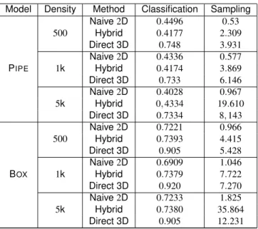
![Figure 11. Quality of the sampling distribution generated with a naive 2D method (blue), with our hybrid method (red), and with the 3D direct method of [4] for P IPE](https://thumb-eu.123doks.com/thumbv2/123doknet/13407732.406844/7.918.158.746.123.541/figure-quality-sampling-distribution-generated-method-hybrid-method.webp)
Documents relatifs
Introduced by Gunter Pauli, the Blue Economy, namely bio-inspired industrial ecology or self-profitable circular economy, is a remarkable example of the way the knowledge flow
maximum envelope amplitude of the stacked signals as a function of reduction velocity (slowness) and profile azimuth, for frequency band FB2.. This calculation corresponds to the
Figure 8 shows the maximum envelope amplitude of the stacked signals as a function of reduction velocity (slowness) and profile azimuth, for frequency band FB2.. This
Our method can generate distributions with sample attributes that are not direct functions of the underlying domains, such as more natural biological distribution
¹GEOTOP, University of Quebec in Montreal, Canada, ²IMPMC, Sorbonne Université, France, ³Mines ParisTech, PSL Research University, France, ⁴Center for Research on the Preservation
L’archive ouverte pluridisciplinaire HAL, est destinée au dépôt et à la diffusion de documents scientifiques de niveau recherche, publiés ou non, émanant des
Another facet of the elegant link between random processes on graphs and Laplacian-based numerical linear algebra is un- covered: based on random spanning forests, novel Monte-
Pléiades’ VHSR images thus appear as a relevant tool for the characterization of these production systems, provided that these images are acquired at different
