HAL Id: hal-01543136
https://hal.archives-ouvertes.fr/hal-01543136
Submitted on 20 Jun 2017HAL is a multi-disciplinary open access archive for the deposit and dissemination of sci-entific research documents, whether they are pub-lished or not. The documents may come from teaching and research institutions in France or abroad, or from public or private research centers.
L’archive ouverte pluridisciplinaire HAL, est destinée au dépôt et à la diffusion de documents scientifiques de niveau recherche, publiés ou non, émanant des établissements d’enseignement et de recherche français ou étrangers, des laboratoires publics ou privés.
Improving landscape connectivity for the Yunnan
snub-nosed monkey through cropland reforestation using
graph theory
Wenwen Li, Céline Clauzel, Yunchuan Dai, Gongsheng Wu, Patrick
Giraudoux, Li Li
To cite this version:
Wenwen Li, Céline Clauzel, Yunchuan Dai, Gongsheng Wu, Patrick Giraudoux, et al.. Improving landscape connectivity for the Yunnan snub-nosed monkey through cropland reforestation using graph theory. Journal for Nature Conservation, Elsevier, 2017, 38, pp.46 - 55. �10.1016/j.jnc.2017.06.002�. �hal-01543136�
Improving landscape connectivity for the Yunnan snub-nosed monkey through
cropland reforestation using graph theory
Wenwen Li
a,b, C
é
line Clauzel
b,c*, Yunchuan Dai
b,d, Gongsheng Wu
b, Patrick Giraudoux
b,f, Li Li
b,*a School of Urban Management and Resource Environment, Yunnan University of Finance and Economics, Kunming 650221, China b Department of Wildlife Management and Ecosystem Health, Yunnan University of Finance and Economics, 237 Long Quan Road,
Kunming 650221, China
c LADYSS, UMR7533-CNRS, University Paris Diderot, Sorbonne Paris Cité 75013, Paris, France d School of Tourism and Geographical Science, Yunnan Normal University, Kunming, 650500 China
f Chrono-Environnement, UMR 6249 CNRS, University of Bourgogne Franche-Comté, and Institut Universitaire de France16 route de
Gray, 25030 Besançon, France
Abstract: Habitat fragmentation is a threat to biodiversity because it restricts the ability of animals to move. Maintaining landscape connectivity could promote connections between habitat patches, which is extremely important for the preservation of gene flow and population viability. This paper aims to evaluate the landscape connectivity of forest areas as it relates to the conservation of the Yunnan snub-nosed monkey (Rhinopithecus bieti), an emblematic and endemic endangered primate species. Specifically, this study seeks to model ways to improve connectivity via cropland reforestation scenarios which incorporate graph theory and genetic distances. The connectivity improvement assessment is performed at two nested scales. At the regional scale, the aim is to quantitatively assess the gain in connectivity from different reforestation scenarios, in which croplands are replaced by different kinds of forest habitats. At the local scale, the goal is to prioritize and to locate croplands based on the gain in connectivity that they would provide if they were reforested. The results indicate that the four reforestation scenarios have different impacts on connectivity; the fourth scenario, in which reforestation is accomplished with plant species that provide optimal monkey habitat, yields the greatest increase in connectivity (+24% versus less than +2% for the others). Prioritization of the 1482 cropland patches shows that the 10 best patches increase connectivity from 0.04% to 9.1% as the isolation threshold distance increases. This kind of graph theoretic approach appears to be a useful tool for connectivity assessment and the development of conservation measures for species impacted by human activities.
Introduction
Human activities generate land use and cover change (LUCC) that may significantly affect natural habitats and, consequently, species viability (Foley et al., 2005). Since the beginning of the 20th century, the acceleration of LUCC has resulted in habitat loss for species of high conservation value, and this acceleration has been particularly strong in China over the last two decades, leading to a reduction in natural habitats (Liu et al., 2003). Many studies have focused on the impacts of urbanization on the environment (Liu et al., 2000), the conversion of natural habitats to cropland also has important consequences, such as pollution, biodiversity loss and habitat fragmentation (Millennium Ecosystem Assessment, 2005a). Habitat fragmentation is a landscape-level spatial process that generates patch-level consequences such as a decrease in habitat patch size and an increase in patch isolation (Fahrig, 2003), and this process is considered a major threat to species viability because it reduces landscape permeability to wildlife movements and gene flow (Cushman et al., 2006; Forman and Alexander, 1998). The maintenance and/or improvement of landscape connectivity, which facilitates the movement of animals among resource patches (Taylor et al., 1993), is thus a major issue facing the preservation of population viability, especially for species that depend on large habitats or on a high degree of connectivity between habitats. The distribution and the survival of primates, for instance, are directly influenced by landscape integrity and connectivity (Anzures-Dadda and Manson, 2007; Arroyo-Rodriguez and Fahrig, 2014).
Over the last decade, many studies have focused on improving and restoring landscape connectivity for species conservation (Bodin and Saura, 2010; Briers, 2002; Clauzel et al., 2015a; Dalang and Hersperger, 2012; Etienne, 2004; Hodgson et al., 2011; McRae et al., 2012), and among the methods used, network analysis based on graph theory is one of the most promising because it offers an interesting compromise between the amount of input data and information about ecological processes (Urban and Keitt, 2001; Calabrese and Fagan, 2004). Graph-based methods are used to model the ecological networks of species, generally to represent the trophic interactions between species in an ecosystem. Here, we use graph modelling to represent the spatial connectivity between habitat patches of a single species, which allows us to analyse both the structural and functional aspects of landscape
networks by integrating species behaviour. A graph is a set of nodes corresponding to the habitat patches of a given species that are connected by links representing potential movements between patches (Galpern et al., 2011). Landscape graph analysis is often used to quantify potential connectivity by means of connectivity metrics (Foltête et al., 2012a), to identify the most important landscape elements (patches or corridors) for preserving connectivity (Baranyi et al., 2011; Bodin and Saura, 2010; Crouzeilles et al., 2013; Erős et al., 2011; Jordán et al., 2003; Saura and Rubio, 2010) or to test different scenarios to improve connectivity. This last goal can be achieved by increasing the size or the quality of existing habitat patches or corridors (Etienne, 2004) or by creating new habitat patches or corridors through landscape restoration (Benedek et al., 2011; Clauzel et al., 2015ab; García-Feced et al., 2011; Zetterberg et al., 2010; Hodgson et al., 2011; McRae et al., 2012).
The aim of this paper is to improve the connectivity of forest networks by proposing different reforestation scenarios, and we use a method that combines graph theory and genetic distances to model the landscape network of a given species. The analysis is focused on the connectivity of high-altitude coniferous forests in Yunnan (China), which have a high value in biodiversity (Yang et al. 2004). The restoration of this ecosystem could benefit to many species living in this habitat, especially the Yunnan snub-nosed monkey (Rhinopithecus bieti). This primate species is an important conservation target because of its endemism and the critical size of its population, which is fragmented into 15 groups. Indeed, the species is highly threatened by growing urbanization and, most importantly, the conversion of forests for cropland, which causes habitat fragmentation and isolation (Xiao et al., 2003). Some studies (Li et al., 2014; Wong et al., 2013) have highlighted the importance of preserving or restoring the corridors between habitat patches to enable monkey movements.
The present study focuses on improving the quality of potential snub-nosed monkey corridors by proposing different reforestation scenarios, which are focused solely on croplands located in the corridors because their restoration is considered easier and more feasible compared to other land cover types. The analysis is conducted at two nested scales, regional and local, that are recognized as important to the distribution and abundance of monkeys (Anzures-Dadda and Manson,
2007). At the regional scale, this research assessed the improvement in connectivity under our cropland reforestation scenarios as differentiated by the type of forest plant species selected for use. At the local scale, we prioritized the cropland patches according to the gain in connectivity that they would provide if they were reforested and to consequently identify the best locations for creating new habitat patches. The results are a useful guide for the implementation of conservation measures, such as habitat restoration, for the Yunnan snub-nosed monkey and, more generally, for threatened species with discrete distributions due to habitat fragmentation.
2. Materials and methods
2.1. Materials
2.1.1. Study area
The study area (Fig. 1) is located in northwest Yunnan Province in the Three Parallel Rivers region (between 29.020 N, 98.038 E in the north and 25.053 N, 99.022 E in the south), which is one of the most ecologically significant areas of China in terms of biodiversity, and covering approximately 17000 km2 across four counties in Yunnan (Deqin, Weixi, Lanping, and Lijiang). The elevation of the study area varies from 1200 m to 5500 m with the northern part being higher (3900 m on average compared to 2900 m in the southern part). Land cover varies greatly between the north and south; the northern part is dominated by subalpine coniferous forest while the southern part contains mixed coniferous and broadleaf forest. In addition, land cover in the south is more fragmented due to a higher density of human activities, such as infrastructure and intensive agriculture.
2.1.2. Study species
The Yunnan snub-nosed monkey is one of the most endangered animal species endemic to China. It lives in inaccessible mountains between 1800 m and 4513 m, one of the most extreme environments for any non-human primate (Long et al., 1996), and its habitat consists in an archipelago of high-altitude coniferous forest patches (Fig. 1) (Li et al., 2006; Wang et al., 2011; Xue et al., 2011). The population is approximately 2500 individuals living in 15 isolated groups (12 groups in Yunnan and 3 groups in Tibet) (Wong et al., 2013), and the number of individuals in a single monkey group ranges between 50 and 200 (Long et al., 1996). The main areas of occupancy are the Baima Mountains (groups 6-10) and the Laojun Mountains
(groups 11 and 12). Since the 1950s, suitable habitats (dark coniferous forest, mixed coniferous and broadleaf forest, and oak patches) have been decreased by over 30%, and the average patch size has been reduced from 15.6 km2 to 5.4 km2 (Xiao et al., 2003). Duo to this reduction in suitable habitats, it is difficult for species to move among resource patches, but it can also prevent genetic exchange between populations, making the species more vulnerable to extinction. (Xiao et al., 2003; Li et al., 2014; Liu et al., 2009).
Fig. 1. Study area and locations of monkey groups in Yunnan Province (China). Land cover was classified into five broad categories corresponding to snub-nosed monkey preferences (Li et al., 2014). The monkey groups 1 to 3 are located further north in the Tibet Autonomous Region.
During the day, the snub-nosed monkey spends most of its time feeding, moving and resting. According to several surveys (Kirkpatrick et al., 1998; Ren et al., 2008; Ren et al., 2009), the daily travel distance varies between 350 m and 3000 m with an average of approximately 1500 m, but dispersal events are not well known, especially in terms of the coverage of extreme distances (Grueter, 2003).
2.1.3. Land cover data
Land cover data were obtained from a supervised classification on SPOT-5 images (Institute of Forest Nature Conservancy’s China programme. All data were geo-corrected in ERDAS 9.2 with a root-mean-square (RMS) error <1. Inventory and Planning, Yunnan, 2012) with ground-truthing by the Conservation Information Centre of The
Land cover was classified into five categories (Table 1) according to the observed preferences of the Yunnan snub-nosed monkey (Clauzel et al., 2015b; Li et al., 2007; Li et al., 2006; Wang et al., 2011; Wu et al., 2005; Zhang et al., 2016) and rasterized at a resolution of 50 m. The
elevational distribution of each land cover type was derived from a 30 m-resolution DEM resampled to 50 m using a bilinear interpolation of the Chinese Geospatial Data Cloud (http://www.gscloud.cn/).
2.1.4 Genetic distance data
The genetic distances between pairs of monkey groups were obtained from the studies of Liu et al. (2007, 2009), in which DNA was extracted from 203 faecal samples, 2 muscle samples and 2 blood samples from 157 individuals from 11 monkey populations (Group1, G3, G4, G5, G6, G7, G9, G10, G11, G13, and G15). This study sequenced 401 bp of the hyper variable I (HVI) segment from the mitochondrial DNA control region (CR) of those samples and genotyped them by microsatellite loci. Finally, 52 variable nucleotide sites were selected, and 30 haplotypes were defined to estimate genetic diversity. A hierarchical analysis of molecular variance was then performed to compare genetic diversity among different groups of Yunnan snub-nosed monkey (Liu et al., 2007).
Table 1
Land cover was classified into five habitat types according to monkey preferences. The elevation range of every habitat type was selected from a digital elevation model, and the cost values for each category were obtained from Li et al. (2014).
Habitat type Land cover type Elevation range
unit (m) Cost value
Optimal Armand pine and hemlock, fir-spruce forest, coniferous broad-leaved mixed forest
2250-4730
1
Suboptimal sclerophyllous evergreen broad-leaved forest,
shrub-dominated land
1220-5240
10
Suitable cold coniferous forest, sub-alpine meadow, broad-leaved forest
1310-4950
70
Unfavourable warm coniferous forest (Yunnan pine forest), hot dry savanna, sparse shrub grass
1200-5490
90
Highly unfavourable cropland, settlements, water body, barren land
1215-5410
100
2.2. Methods
The method had three main steps. First, we modelled the landscape network of the snub-nosed monkey using graph theory and genetic distances, and we then assessed the impact of different cropland reforestation scenarios on connectivity at the regional scale. Finally, we prioritized croplands according to the gain in connectivity that they
would provide if they were reforested.
2.2.1. Modelling the landscape network of the snub-nosed monkey
In the study, we focused on modelling the snub-nosed monkey landscape network at the scale of individual dispersal.
The nodes of the graph were defined following the concept of “metapatches” developed by Zetterberg et al. (2010) and previously used in Clauzel et al. (2015b) for the snub-nosed monkey. This concept is based on a life traits, and the functional definition of habitat patches depends on the ecological process being considered (Theobald, 2006). At the daily scale and in a fragmented habitat, a graph node is defined as a single habitat patch in which an individual finds all of its daily resources (typically foraging). At the dispersal scale, a graph node is defined as a set of habitat patches connected by daily movements; it is assumed that the species can move within the metapatches without having to overcome major barriers to foraging (Blazques-Cabrera et al., 2014). A metapatch contains both optimal habitat and the surrounding matrix, and the connections between these metapatches potentially support natal dispersal and genetic exchange, which are recognized as key factors for population viability.
The metapatch-based approach implies the creation of two successive graphs (Clauzel et al., 2015), the first of which identifies connected habitat patches at the daily scale, and each graph node corresponds to a single optimal habitat patch (Armand pine, hemlock, coniferous broad-leaved mixed forest, and fir-spruce forest). The subparts of the graph (termed “components”), which are composed of the sets of connected habitat patches, correspond to the areas where monkeys can move during a day. These components, which are defined at the daily scale, will be the nodes (termed “metapatches”) in the second graph, which represents the landscape network at the dispersal scale. In this graph, the new components, i.e., the sets of connected metapatches, are the areas where monkeys can move during a year. As the snub-nosed monkey often prefer large habitat patches, each optimal habitat patch was associated with a quality value depending on its size. For a given metapatch, the quality value was equal to the total area of optimal habitat inside.
The links between nodes were defined using cost distances, which are considered more realistic than Euclidean distances. Each pixel of a land cover map was assigned a cost according to its resistance to monkey movements, and these cost values were based on the study by Li et al. (2014), in which several combinations of least-cost distances were compared to the genetic distances between monkey groups. According to this study, optimal habitat was assigned a cost of 1, suboptimal habitat a cost of 10, suitable elements for movements a cost of 70, unfavourable elements a cost of 90 and highly
unfavourable a cost of 100 (Table 1).
Generally, the graph modelling a landscape network is thresholded using the dispersal distance of the studied species to remove links that are too long and/or too costly to be potentially used by individuals (Saura and Pascual-Hortal, 2007), but in our study, the dispersal distance of the snub-nosed monkey was poorly known because dispersal events are difficult to observe (Grueter, 2003). Consequently, the dispersal distance was derived from the relationship between the genetic distances and the cost distances between monkey groups. Genetic distance was plotted against cost distance, and 5 model functions (power, linear, exponential, log and polynomial) were fitted to the data. The Akaike information criterion (AIC) was used to select the best model, and the selected dispersal distance was the minimal cost-distance at which the genetic distance levelled off in the best model, assuming that groups were isolated by distance and contact between groups, if any, was minimized beyond this threshold.
As the analysis focuses on the corridors, the potential corridors between monkey groups were mapped using least-cost distances, and the cost values were assigned to each land cover type using Linkage Mapper (McRae and Kavanagh, 2011). This tool created a map of cumulative movement resistance between core areas (here, monkey groups), and cumulative cost distances were then classified into five classes by the quantile method. Only the first class was kept, and it was assumed to be the most likely used corridor, i.e., the least costly.
2.2.2. Protocol for evaluating the effect of potential reforestation on connectivity
At the regional scale, the analysis quantifies changes in the overall landscape connectivity induced by the reforestation of croplands in the corridors, and four potential scenarios that differed in the type of plant species selected for reforestation were evaluated. To make the reforestation scenarios realistic, we also considered the elevational distribution of every land cover type (Table 1).
-C1: croplands are reforested with plant species constituting unfavourable habitat for monkeys such as Yunnan pine forest at lower altitudes and sparse shrub grass at higher elevations (cost value is 90);
-C2: croplands are reforested with plant species constituting suitable habitat such as sclerophyllous evergreen broad-leaved forest and other shrub-dominated
land (cost value is 70);
-C3: croplands are reforested with plant species constituting suboptimal habitat such as cold coniferous forest and broad-leaved forest (cost value is 10);
-C4: croplands are reforested with plant species constituting optimal habitat such as fir-spruce at higher altitudes and replaced by the best possible suboptimal habitat (such as shrub-dominated forest) if the elevation of the cropland is below the elevation of the optimal habitat (cost value is 1 for optimal habitat and 10 for suboptimal habitat).
For each of these scenarios, the land cover map was modified, and a new graph was built using the same parameters for defining nodes and links at the dispersal scale. Then, a global connectivity metric was calculated for each of the parameters and compared to the initial state to assess their contribution to the current connectivity (C0).
At the local scale, the analysis provides a more accurate assessment by identifying the most strategic cropland patches in the corridors for improving connectivity, which is based on the patch addition process developed by Foltête et al. (2014) that identifies the best locations for new habitat patches. The process begins by computing a global metric that quantifies the connectivity of the initial network and then each cropland patch in the corridors is considered a new habitat patch, and the metric is computed again. After all cropland patches are tested, the one that provided the greatest increase in connectivity is identified, and the process is repeated until the desired number of new patches is reached. As a first step, we arbitrarily decided to add 10 new patches to reduce the computation time. If the resulting curve of the connectivity improvement showed an increase for the tenth patch, the analysis could be performed again with more added patches.
At these two scales, the connectivity assessment was based on the probability of connectivity index (PC)
developed by Saura and Pascual-Hortal (2007). The PC index is a global metric given by the expression:
PC = (∑n
i=1 ∑nj=1aiajp*ij)/A² (1)
where ai and aj are the areas of habitat patches i and j; A is
the total landscape area (comprising both habitat and non-habitat); and p*
ij is defined as the maximum product
probability of all possible paths between patches i and j (including single-step paths). Pij is determined by an
exponential function such that:
pij= exp(-αdij) (2)
where dij is the least-cost distance between these
patches, and α (0<α<1) expresses the intensity of the decrease in the dispersal probabilities resulting from this exponential function (Foltête et al., 2012a).
All analyses were performed using Graphab 2.0 software (Foltête et al., 2012a) (Software available at
http://thema.univ-fcomte.fr/productions/graphab/en-home.html), but the corridors were identified with the Linkage Mapper Toolkit for ArcGIS.
3. Results
3.1. The current snub-nosed monkey landscape
network
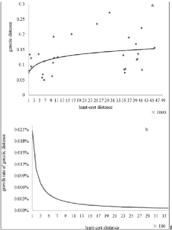
To identify the graph components at the dispersal scale (i.e., metapatches), we compared genetic distances and cost distances between monkey groups to define a threshold for removing the longest links. The log and polynomial models had lower AIC values with △AIC<2, so
they can be considered equivalent according to the usual
AIC criterion. The log function was considered more
realistic as a description of the relationship between genetic distances and cost distances since it was increasing and monotonic (the polynomial function first shows increasing genetic distances with increasing cost distances followed by decreasing distances, which does not make sense biologically).
Table 2
Genetic distance as a function of least-cost distance (* is the optimal function). y represents genetic distance, and x represents least-cost distance.
Function type Expression R2 AIC Sample size
power y=0.0134𝑥0.224 0.42 45.98 35
linear y=2E-06x+0.084 0.23 -101.26 35
exponential y=0.072𝑒2𝐸−05𝑥 0.27 54.25 35
*log y=0.021ln(x)-0.074 0.34 -106.45 35 polynomial y=-2E-10x2 +9E-06x+0.057 0.38 -106.64 35
Fig. 2 shows the data, the selected log model (Fig. 2a) and its derivative function (Fig. 2b) (y = 0.021/x). We arbitrarily chose a cost distance threshold of 1200 (approximately 70% of the integral of the curve) to identify graph components at the dispersal scale; this distance was considered an approximation of the dispersal distance of the snub-nosed monkey. However, as the curve does not level off at greater distances, several other distances were tested to evaluate model sensitivity to this threshold.
Fig. 2. Genetic distance and least-cost distance (a). Cost values came from the study by Li et al. (2014a), and genetic values were from Liu (2010); growth of genetic distance with least-cost distance (b).
Modelling the landscape network at the dispersal scale first required this network to be modelled at the daily scale to define metapatches. In the first graph (Fig. 3a), the nodes were defined as optimal habitat patches, and the links were thresholded at the mean daily travel distance. This landscape network contains 1466 nodes and 314 components, and these nodes correspond to daily resource patches where monkeys can find food and rest. Then, a second graph was constructed to represent the landscape network at the dispersal scale by converting these 314 components into 314 nodes (also called “metapatches”), and in this second graph, the links were thresholded at 1200 cost units, which corresponded to the
approximate dispersal distance. This graph contains 314 nodes grouped into 111 components ranging from 2 to 5756 km2 (147 km2 on average) and 258 links (Fig. 3b). The largest component occupies a large portion of the north and centre of the study area (Baima Snow Mountains) and is home to 6 monkey groups, and the second largest component is the Laojun Mountains in the southeast with two monkey groups. In the northwest of the study area, a smaller component has one monkey group, which appears isolated from the others (but is potentially connected to the Tibetan groups). Finally, three isolated monkey groups are present at the southern extremity of the study area, which appears more fragmented due to a lower density of favourable landscape elements.
Fig. 3. The graphs modelling the landscape network of the snub-nosed monkey at the daily scale (a) and at the dispersal scale (b). In a, nodes were defined as optimal habitat patches, and links were thresholded at the mean daily distance. In b, nodes were defined as metapatches, which corresponded to the components defined in a, and links were thresholded at the dispersal distance.
A least-cost corridor was mapped between each monkey group (Fig. 4), the width of which varies according to the density of suboptimal and suitable habitat, i.e., areas with the lowest resistance values. The corridor is
largest in the middle part of the study area due to a higher density of favourable landscape elements in the Baima Snow Mountain Reserve, but it is narrower in the southern part, where suboptimal and suitable habitats are few and the degree of fragmentation is very high.
Fig. 4. Corridors between monkey groups based on the least-cost distance. The agricultural lands inside the corridor were selected to improve landscape connectivity.
3.2. Evaluation of the reforestation scenarios
(regional scale)
The analysis is focused on improving the quality of the corridors through cropland reforestation. There are 1482 cropland patches in the corridors that are mostly located in the southern half of the study area where monkey habitat is highly fragmented. The altitude of the croplands
is compatible with the altitude of each habitat type, so the four reforestation scenarios were not limited by altitude and were considered feasible.
The comparative analysis of the four scenarios shows that the changes in global connectivity vary greatly (from +0.03% to 24.05%) depending on the type of vegetation used for reforestation (Table 3). The first two scenarios minimally improve connectivity (+0.03% for C1 and +0.81% for C2) and have no impact on the structure of the graph, while the third scenario slightly improves connectivity (+2.37%). The improvement in the quality of the landscape matrix causes the four graph components to merge. The C4 scenario most increases connectivity (+24.05%); in this scenario, the number of metapatches and components at the dispersal scale are fewer but larger due to the creation of new habitat patches in the daily scale graph. The mean metapatch area is 11.41 km² for the C4 scenario compared with 10.7 km² for the initial state, and the mean graph component area increases by 4 km² (from 147 km² for the initial state to 151 km² under the C4 scenario).
3.3. Prioritization of cropland patches (local scale)
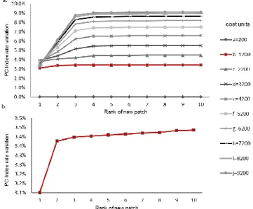
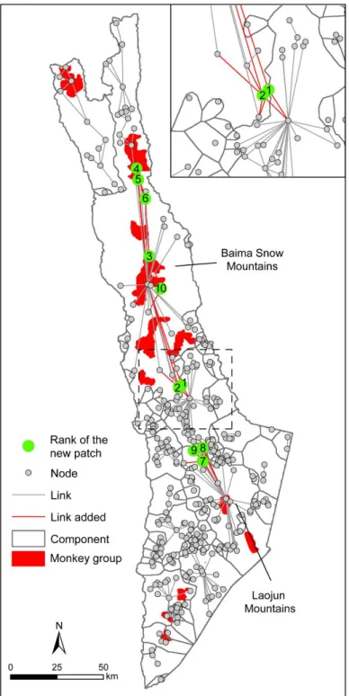
To refine the analysis, the 1482 cropland patches located in the corridors were prioritized according to the gain in connectivity after reforestation with optimal habitat (i.e., transformation into a new habitat patch). In addition to the previously used cost distance of 1200, several other distances ranging from 200 to 9200 cost units were tested to evaluate the sensitivity of the results (Fig. 5a). If the rate of variation in the PC index increased with the distance (which varied from 0.04% for 200 cost units to 9.1% for 9200 cost units), the shapes of the curves were quite similar. Globally, the rate of variation reached a maximum with the addition of the third patch, regardless of the cost distance, so we focused the analysis on the 1200 cost distance (Fig. 5b). The 10 new habitat patches provided little improvement in global connectivity (+3.5%), and among these new habitat patches, 7 cropland patches (the 1st to 6th and the 10th patches) were located in the largest component (Fig. 6). The first two patches are next to the border between two components and reconnect them, so the combination of these two patches provides the largest increase in connectivity (+3.38%) because it allows the largest component to become even larger. The third, fourth, fifth, sixth and tenth new patches increase the density of connections between the central and northeast parts, and the 3 other patches (7th to 9th) are located further south and reconnect the Laojun Mountains to the Baima Snow Mountains.
Table 3
Results of the analysis applied at the region scale. The table contains both the connectivity values of each scenario (C1, C2, C3, C4) and the rate of variation of these values compared to the current situation (C1/C0; C2/C0; C3/C0; C4/C0).
Scenario PC a LNb CNc MNd MSMe MSCf
C0 (current) 1.639E-03 258 111 314 10.70 147 C1 (reforested with unfavourable habitat) 1.640E-03 258 111 314 10.70 147
C1/C0 0.03% 0 0 0 0 0
C2 (reforested with suitable habitat) 1.65E-03 257 110 313 10.73 148 C2/C0 0.81% -0.39% -1 -0.32% 0.32% 0.68% C3 (reforested with suboptimal habitat) 1.678E-03 251 107 305 11.01 153
C3/C0 2.37% -2.79% -4 -2.95% 2.95% 4.08% C4 (reforested with optimal habitat) 2.158E-03 251 108 306 11.41 151
C4/C0 24.05% -2.79% -3 -2.55% 6.65% 2.72%
a The distance parameter of the probability of connectivity (PC) was set to a cost distance of 1200. b LN: number of links
c CN: number of components d MN: number of metapatches e MSM: mean metapatch size in km2 f MSC: mean component size in km2
Even if the improvement in global connectivity is weak, these 10 new habitat patches appear to be important because they potentially reconnect two nature reserves (Baima and Laojun) and five monkey groups (Fig. 6). They also increase the density of nodes and links in the network, making it more robust in case of disturbance.
Fig. 5. Curves showing the increase in connectivity provided by new habitat patches at different distance thresholds (a). Detail of the 1200 cost distance curve (b). The degree of connectivity is assessed by the PC index metric, and values represent the rate of variation in the initial PC index value resulting from the addition of each new patch.
4. Discussion
This paper proposes an integrative approach to study the effects of landscape fragmentation on the movement and population viability of the Yunnan snub-nosed monkey. Specifically, the main objective was to assess the impact of the potential reforestation of croplands on connectivity.
4.1.
Integrating
functional
connectivity
in
conservation studies
Graph modelling appears to be a relevant approach to integrate functional connectivity in landscape network analysis (Calabrese and Fagan, 2004). The role of species preferences in landscape movements is taken into account through the use of cost distances, and the graph is associated with a threshold distance for removing links that are too long and/or too costly based on the movement capacities of the studied species. Generally, graph studies are focused on dispersal distance, which is a key parameter in the ecological processes that lead to species persistence, but in these studies, scale mismatch often occurs due to discrepancies between the scale of the definition of habitat patches and the scale of the dispersal. Indeed, habitat patches are traditionally defined as contiguous cells of particular land cover classes (Zetterberg et al., 2010), and in this case, they may correspond to a restricted foraging area (i.e., a local and daily process). The real foraging area can encompass a set
of several discrete patches, and in this case, the links between patches are only used for daily movements and can be misrepresented as exclusively potential dispersal routes (i.e., vectors for regional and annual ecological processes).
Fig. 6. Location of the ten best cropland patches that maximize connectivity. The rectangle shows the first two new patches in detail.
Here, our approach attempts to address this mismatch by defining habitat patches at two scales, annual home ranges and routes for long-distance dispersal. Hence, “metapatches” correspond to the set of habitat patches connected at the daily scale and contain all the resources
needed throughout the year (Zetterberg et al., 2010). Links between metapatches are assumed to represent routes for more exceptional dispersal events that can connect strongly isolated groups.
However, this kind of nested approach requires the daily and dispersal distances of the species under consideration to be precisely known. In the case of the Yunnan snub-nosed monkey, field surveys have provided information about its mean daily travel distance but not its dispersal distance (i.e., the distance that rare dispersers might reach during a random excursion) due to the difficulty of observing this process. Thus, our study estimated this distance based on the relationship between the genetic distances and cost distances between monkey groups, but as the results are highly dependent on this approximation, they to be confirmed by field surveys. Another caveat is that this genetic distance approach does not reveal the actual network used by the snub-nosed monkey; rather, it more likely reveals the one used in the past to reach the genetic structure of the population as currently estimated. To increase the degree of realism of the graph modelling, each habitat patch has a quality value depending on its size. This value is an indicator of the demographic potential which is intrinsic to the patch and independent of the graph (Urban and Keitt, 2001). This parameter can be considered as a proxy to integrate source-sink interactions in graph modelling without the need of in-depth knowledge about species behaviour.
With those cautions in mind, our results can inform which field studies and areas should be prioritized to collect relevant information, which is a key challenge in conservation research. Furthermore, as graphs provide a spatially explicit representation of landscape networks, they can be an interesting tool to communicate the meaning of and issues related to connectivity to landscape managers (Bergsten and Zetterberg, 2013). Last but not least, this multiscale approach has the potential to be used for other species whose optimal habitat is patchily distributed and where long distance dispersal should be rare. This approach may apply to a very large and increasing number of species in the context of increasing habitat fragmentation worldwide.
4.2 Implications for species conservation
Similar to most primates (Estrada et al., 2017), the Yunnan snub-nosed monkey is threatened by the loss and fragmentation of its habitat due, in large part, to
agricultural expansion. Current conservation measures have been successful applied to stabilize and even slightly increase snub-nosed monkey populations, but their long-term viability remains uncertain, especially for the groups living in the highly fragmented south area and in the context of increasing agricultural encroachment. Consequently, facilitating long-distance movements is particularly important.
Our graph-based approach allows potential areas for reforestation to be localized and prioritized to improve connectivity. Reforestation scenarios were focused on connecting current monkey groups by corridors to promote gene exchange and thus population viability. Combining presence data and graph modelling improves the ecological significance of the results and provides guidance for future field surveys. Only cropland patches were tested in the scenarios because this kind of reforestation has been implemented in China since 1990 (Grain for Green project), even though the aim was different than ours (reducing, e.g., soil erosion on steep slopes). In this case, it will take several decades of reforestation before the vegetation is sufficiently developed to become optimal snub-nosed monkey habitat. Furthermore, we did not consider the feasibility of the scenarios from a social perspective. To make reforestation measures more realistic, we should learn from the experiences of the Grain for Green project, such as providing financial compensation for farmers and guiding them to develop forestry investment instead of extractive uses.
The results of our study show that the last scenario (C4), in which reforestation was theoretically accomplished with optimal habitat plant species, was the only one that provided a large increase in connectivity (+24% compared to less than 2% with the others). The creation of new habitat patches would lead to an increase of the mean size of the graph components, meaning that monkeys could travel greater distances during dispersal events, but a comparison of the C3 and C4 scenarios shows that this increase is stronger under C3 (suboptimal) than C4 (Table 3). This seemingly contradictory result is possibly due to the location of the croplands being converted into optimal habitat patches as some are totally isolated from the other habitat patches, leading to the creation of a new component around each former cropland patch in the C4 scenario. The size of these new components is very small and thus decreases the average size, whereas the isolation of these new habitat patches makes them useless for
species conservation. These results suggest that reforesting all croplands regardless of their location might not be effective, especially because some of are too far from an existing patch of optimal habitat. In addition, it does not seem realistic to reforest all croplands because they are sources of food and income for farmers in those areas. Consequently, the identification of the most strategic croplands for potential reforestation measures seems to be a more relevant approach. Finally, the two scales of analysis are complementary. The regional-scale analysis provides a global evaluation, but it might not be realistic (too costly, poor approval from farmers, isolation of new habitat patches, etc.) while the local-scale analysis provides a more precise evaluation that could guide habitat restoration in the field.
5. Conclusion
Even if our approach was focused on a single animal species, the results can benefit to other species living in high-altitude coniferous forests, since the Yunnan snub-nosed monkey could be considered as an umbrella species. But this graph-based approach can also be applied to other species living in fragmented habitats by adapting the ecological parameters (habitat definition, resistance to movement, and distance capacities). As the populations of 75% of primate species are in decline (Estrada et al., 2017), this approach can help identify priority habitats for conservation and/or restoration at a spatio-temporal scale consistent with long-term population viability.
Acknowledgement
This study has been supported by the National Key Technology R&D Program of China (2013BAD03B02) and the National Natural Science Foundation of China (NSFC no: 31100351), the University of Finance and Economics, Kunming and the Key lab of hazard risk management and Wildlife Management and Ecosystem Health center. Studies have been carried out with the support of the GDRI Ecosystem Health and Environmental Disease Ecology
http://gdri-ehede.univ-fcomte.fr. We also thank countless people who have regularly provided invaluable support and aid during our field expeditions.
References
Arroyo-Rodríguez,V., Fahrig, L., 2014. Why is a landscape perspective important in studies of primates? American Journal of Primatology. 901–909.
Anzures-Dadda, A., Manson, R., 2007. Patch- and landscape-scale effects on howler monkey distribution and abundance in rainforest fragments. Animal Conservation.10, 69-76.
Baguette, M.,Blanchet, S., Legrand, D., Stevens, V. M., Turlure. C., 2013. Individual dispersal, landscape connectivity and ecological networks. Biological Reviews Of The Cambridge Philosophical Society 88:310–326.
Baranyi, G., Saura, S., Podani, J., Jordán, F., 2011. Contribution of habitat patches to network connectivity: redundancy and uniqueness of topological indices. Ecological Indicators.11, 1301– 1310.
Benedek, Z., Nagy, A., Rácz, I. A., Jordán, F., Varga, Z., 2011. Landscape metrics as indicators: Quantifying habitat network changes of a bush-cricket Pholidoptera transsylvanica in Hungary. Ecological Indicators.11, 930–933.
Bergsten, A., Zetterberg, A., 2013. To model the landscape as a network: A practitioner’s perspective. Landscape and Urban Planning 119, 35–43.
Blazquez-Cabrera, S., Bodin, Ö., Saura, S., 2014. Indicators of the impacts of habitat loss on connectivity and related conservation priorities: do they change when habitat patches are defined at different scales? Ecological Indicators. 45, 704-716.
Bodin, Ö., Saura, S., 2010. Ranking individual habitat patches as connectivity providers: integrating network analysis and patch removal experiments. Ecological Modelling. 221, 2393–2405. Briers, R.A., 2002. Incorporating connectivity into reserve selection procedures. Biological Conservation.103, 77-83.
Brooks, C.P, 2003. A scalar analysis of landscape connectivity. Oikos. 102, 433-439.
Bunn, A.G., Urban, D.L., Keitt, T.H., 2000. Landscape connectivity: a conservation application of graph theory. Journal of Environmental Management. 59, 265–278.
Calabrese, J.M., Fagan, F.W., 2004. A comparison-shopper’s guide to connectivity metrics. Frontiers in Ecology and the Environment. 2(10), 529-536.
Clauzel, C., Bannwarth, C., Foltête, J.-C., 2015a. Integrating regional-scale connectivity in habitat restoration: an application for amphibian conservation in eastern France. Journal for Nature Conservation. 23, 98-107.
Clauzel, C., Deng, X., Wu, G., Giraudoux, P., Li, L., 2015b. Assessing the impact of road developments on connectivity across multiple scales: Application to Yunnan snub-nosed monkey conservation. Biological Conservation. 192, 207-217.
Crouzeilles, R., Lorini, M.L., Grelle, C.E.V., 2013. The importance of
using sustainable use protected areas for functional connectivity. Biological Conservation. 159, 450–457.
Cushman, S., McKelvey, K., Hayden, J., Schwartz, M., 2006. Gene flow in complex landscapes: testing multiple hypotheses with causal modeling. American Naturalist.168, 486–499.
Dalang, T., Hersperger, A.M., 2012. Trading connectivity improvement for area loss in patch-based biodiversity reserve networks. Biological Conservation. 148, 116–125.
Estrada, A., Garber, P.A., Rylands, A.B., Roos, C., Fernandez-Duque, E., Fiore, A.D., Nekaris, K.A.-I., Nijman, V., Heymann, E.W., Lambert, J.E., Rovero, F., Barelli, C., Setchell, J.M., Gillespie, T.R., Mittermeier, R.A., Arregoitia, L.V., Guinea, M. de, Gouveia, S., Dobrovolski, R., Shanee, S., Shanee, N., Boyle, S.A., Fuentes, A., MacKinnon, K.C., Amato, K.R., Meyer, A.L.S., Wich, S., Sussman, R.W., Pan, R., Kone, I., Li, B., 2017. Impending extinction crisis of the world’s primates: Why primates matter. Science Advances 3.
Erős, T., Schmera, D., Schick, R.S., 2011. Network thinking in riverscape conservation – agraph-based approach. Biological Conservation.144, 184–192.
Etienne, R.S., 2004. On optimal choices in increase of patch area and reduction of interpatch distance for metapopulation persistence. Ecological Modelling.179, 77-90.
Foltête, J.-C., Girardet, X., Clauzel, C., 2014. A methodological framework for the use of landscape graphs in land-use planning. Landscape Urban Plan. 240–250.
Forman, R.T.T., Alexander, L.E., 1998. Roads and their major ecological effects. Annual Review of Ecology and Systematics. 29, 207C2.
Fahrig, L.,2003. Effects of habitat fragmentation on biodiversity. Annual Review of Ecology, Evolutionand Systematics. 34, 487-515. Foley, J. A., Defries, R., Asner, G. P., Barford, C., Bonan, G., Carpenter, S. R., et al.(2005). Global consequences of land use. Science, 309, 570–574.
Foltête, J.-C., Clauzel, C., Vuidel, G., 2012a. A software tool dedicated to the modelling of landscape networks. Environmental Modelling and Software.38, 316–327.
Galpern, P., Manseau, M., Fall, A., 2011. Patch-based graphs of landscape connectivity: a guide to construction, analysis and application for conservation. Biological Conservation. 144,44–55. García-Feced, C., Saura, S., Elena-Rosselló, R., 2011. Improving landscape connectivity in forest districts: A two-stage process for prioritizing agricultural patches for reforestation. Forest Ecology and Management.261, 154–161.
Grueter, C.C., 2003. Social Behavior of Yunnan Snub-Nosed Monkeys (Rhinopithecus Bieti). University of Zurich (Thesis).
Hodgson, J.A., Thomas, C.D., Cinderby, S., Cambridge, H., Evans, P., Hill, J. K., 2011.Habitat re-creation strategies for promoting adaptation of species to climate change. Conservation Letters. 4,
289–297.
Jordán, F., Báldi, A., Orci, K.M., Rácz, I., Varga, Z., 2003. Characterizing the importance of habitat patches and corridors in maintaining the landscape connectivity of a pholidoptera
transsylvanica (orthoptera) metapopulation. Landscape Ecology.18,
83–92.
Kirkpatrick, R.C., Long, Y.C., Zhong, T., Xiao, L., 1998. Social organization and range use in the Yunnan snub-nosed monkey rhinopitheus bieti. International Journal of Primatology. 19, 13-51. Li, G., Yang, Y., Xiao, W., 2006. Research on biodiversity and threat factors at the habitat of Rhinopithecus bieti. Yunnan Environment Science.25, 15–18 (in Chinese).
Li, G., Yang, Y., Xiao, W.,2007. A study on vegetation types of
Rhinopithecus bieti habitat. Journal of West China Forestry Science.
36, 95–98 (in Chinese).
Li, L., Xue, Y., Wu, G., Li, D., Giraudoux, P., 2014. Potential habitat corridors and restoration areas for the black-and-white snub-nosed monkey Rhinopithecus bieti in Yunnan, China. Oryx Firstview. 1–8. Liu S., Wu C., Shen H., 2000. A GIS-based model of urban land use growth in Beijing, ActaGeogr. Sin55, 407–416(in Chinese).
Liu J., Zhuang D., Luo D., Xiao X., 2003. Land-cover classification of China: integrated analysis of AVHRR imagery and geophysical data. International Journal of Remote Sensing. 24, 2485–2500
Liu, Z., Ren, B., Wei, F., Long, Y., Hao, Y., Li, M., 2007. Phylogeography and population structure of the Yunnansnub-nosed monkey (Rhinopithecus bieti) inferred from mitochondrial control region DNA sequence analysis. Molecular Ecology, 16, 3334–3349. Liu, Z., Ben, B., Wu, R., Hao, Y., Wang, B., Wei, F., Long, Y., Li M., 2009. The effect of landscape features on population genetic structure in Yunnan snub-nosed monkeys (Rhinopithecus bieti)implies an anthropogenic genetic discontinuity. Molecular Ecology. 18, 3831-3846.
Long, Y., Zhong, T, Xiao, L., 1996. Study on geographical distribution and population of the Yunnan snub-nosed monkey. Zoological Research. 17, 437–441 (in Chinese).
McRae, B.H., D.M. Kavanagh, D.M.,, 2011. Linkage mapper connectivityanalysis software. The Nature Conservancy, Seattle.
McRae, B.H., Hall, S.A., Beier, P., Theobald, D.M., 2012. Where to restore ecological connectivity? Detecting barriers and quantifying restoration benefits. PLoS ONE. 7.
Millennium Ecosystem Assessment, 2005a. Eccosystems and Human Well-being: Biodiversity Synthesis. World Resources Institute, Washington, DC.
Ren, B., Li, M., Long, Y., Grüter, C.C., Wei, F., 2008. Measuring Daily Ranging Distances of Rhinopithecus bieti via a Global Positioning System Collar at Jinsichang, China: A Methodological Consideration. International Journal of Primatology. 29, 783–794.
Ren, B., Li, M., Long, Y., Wei, F., 2009. Influence of day length,
ambient temperature, and seasonality on daily travel distance in the Yunnan snub-nosed monkey at Jinsichang, Yunnan, China. American Journal of Primatology. 71, 233–241.
Saura, S., Pascual-Hortal, L.,2007. A new habitat availability index to integrate connectivity in landscape conservation planning: Comparison with existing indices and application to a case study. Landscape and Urban Planning. 83, 91-103.
Saura, S., Rubio, L., 2010. A common currency for the different ways in which patches and links can contribute to habitat availability and connectivity in the landscape. Ecography. 33, 523–537.
Taylor, P.D., Fahrig, L., Henein, K., Merriam, G., 1993. Connectivity is a vital element of landscape structure. Oikos.68, 571–573.
Theobald, D.M., 2006. Exploring the functional connectivity of landscape of landscapes using landscape network. In: Crooks, K.R., Sanjayan, M. (Eds.), Connectivity Conservation, Conservation Biology.
Urban, D., Keitt, T.,2001. Landscape connectivity: a graph-theoretic respective. Ecology. 82, 1205-1218.
Wong, M., Li, R., Xu, M, Long, Y.,2013. An integrative approach to assessing the potential impacts of climate change on the Yunnan snub-nosed monkey. Biological Conservation.158, 401-409. Wu, R., Zhou, R., Long, Y., Du, Y, Wei, X., 2005. Analysis of suitable habitat for Yunnan golden monkey with remote sensing. Remote Sensing Information. 71, 24-28 (in Chinese).
Wang, Y., Xue, Y., Xia, Y., 2011. Landscape pattern and its fragmentation evaluation of habitat of Rhinopithecus bieti in northwest Yunnan. Forest Inventory and Planning.36, 34–37 (in Chinese).
Xiao, W., Deng, W., Cui, L-W., Zhou, R-L., Zhao, Q-K., 2003. Habitat degradation of rhinopithecus bieti in Yunnan, China. International Journal of Primatology. 24, 389-398.
Xue, Y., Li, L., Wu, G., Zhou, Y.,2011.Concepts and techniques of landscape genetics. Acta Ecologica Sinica.31, 1756-1762 (in Chinese). Yang, Y., Tian, K., Hao, J., Pei, S., Yang, Y., 2004. Biodiversity and biodiversity conservation in Yunnan, China. Biodiversity Conservation. 13, 813-826
Zetterberg, A., Mörtberg, U. M., Balfors, B., 2010. Making graph theory operational for landscape ecological assessments, planning, and design. Landscape and Urban Planning.95, 181–191.
Zhang, Y., Li, L., Wu, G., Zhou, Y., Qin, S., Wang, X., 2016. Analysis of landscape connectivity of the Yunnan snub-nosed monkeys (Rhinopithecus bieti) based on habitat patches. Acta Ecologica Sinica. 36, 51-58(in Chinese).
Zhang, J., Wang, T., Ge, J., 2015. Assessing vegetation cover dynamics induced by policy-driven ecological restoration and Implication to soil erosion in southern China. PLoS ONE. 10, e0131352.