HAL Id: hal-02878055
https://hal.laas.fr/hal-02878055
Submitted on 22 Jun 2020
HAL is a multi-disciplinary open access
archive for the deposit and dissemination of
sci-entific research documents, whether they are
pub-lished or not. The documents may come from
teaching and research institutions in France or
abroad, or from public or private research centers.
L’archive ouverte pluridisciplinaire HAL, est
destinée au dépôt et à la diffusion de documents
scientifiques de niveau recherche, publiés ou non,
émanant des établissements d’enseignement et de
recherche français ou étrangers, des laboratoires
publics ou privés.
Time slot modeling of life habits in the elderly for
decision-making support
Damien Brulin, Eric Campo, Clément Lejeune, Daniel Estève
To cite this version:
Damien Brulin, Eric Campo, Clément Lejeune, Daniel Estève. Time slot modeling of life habits in
the elderly for decision-making support. Innovation and Research in BioMedical engineering, Elsevier
Masson, 2020, 41 (6), pp.295-303. �10.1016/j.irbm.2020.06.012�. �hal-02878055�
Time slot modeling of life habits in the elderly for decision-making support
D. Brulina,˚, E. Campoa,˚, C. Lejeunea, D. Est`evea
aLAAS-CNRS, Universit´e de Toulouse, CNRS, UT2J, Toulouse, France
Abstract
This article investigates new steps for the implementation and the utilization of presence indicators to identify dis-placement activities of a person and to model their life habits. This modeling is based on preliminary measures of displacement rate variations over a period of time. A possible time slot division of activities is highlighted by the analysis of these measures, slight variations of slot boundaries could appear from day to day, from person to person. On this basis, we show how to build three new indicators by working from time slot to time slot, in order to detect alerts or drifts from “normal” behavior as soon as possible and in a more reliable way. These indicators include start and end times of time slots, displacement rate and duration of each time slot. The algorithm we propose has been tested in real situations to show its use and relevance. Results are finally integrated in a more ambitious process of detection and automatic decision-making support through the conception of a web interface.
Keywords: behavior modeling, classification, homecare, decision-making support
1. Introduction
The interest to have at our disposal human behavior models was obvious from the beginning of works dedicated to home monitoring of the elderly. Indeed customized identification of life habits appeared to be a solid base to detect changes which may show a sudden risk for the person or a slower change of their health state: unexpected events, dizzy spells, falls, walking speed or physical activity decrease. . . This concept has been to a great extent applied by
5
the authors of this article [1, 2]. It has been further investigated in specialized literature [3, 4, 5, 6, 7] as one of the keystones of risk detection at home.
Using this concept directly with presence indicators seems to be the most concrete implementation [4], by using learning processes. We observe, during the learning phase, a patient’s presence in different strategic locations (living-room, kitchen, bed(living-room, entrance. . . ) in order to determine presence probabilities and standard deviations; these
10
indicators, periodically updated, will allow to define habitual presence rate which will be considered as “normal” for the observed person and so to detect a presence lack or excess, once the initial learning phase is finished. On this basis, a first level of monitoring can be considered which will launch automatic alerts thanks to well-selected living spaces which are reliable indicators of greatly-fixed daily activities. For example, presence rate in the bedroom allows to determine that the time when a person goes to bed and gets up are generally identical from day to day.
15
Elderly monitoring at home, using only movement sensors distributed in different rooms, is a well-known and mature approach nowadays. Indeed, it is already present in commercial offerss1which can be found in telemonitoring,
telecare for home support. However, it is necessary, during execution, to find a procedure to optimize the management of false alarms still relatively numerous. In this article, we will focus on methods and means allowing to reduce false alarms by:
20
• relying more on the identification of the nature of patient’s activities during the day and at night,
˚Corresponding author
Email addresses: dbrulin@laas.fr (D. Brulin), ecampo@laas.fr (E. Campo) URL: clement.lejeune@irit.fr (C. Lejeune)
• using several indicators and their convergences from a decision-making viewpoint,
• offering the opportunity to configure decision rules specific to each person and to each time slot thanks to a web interface.
2. Time slots division
25
We do not question the idea of relying on the presence rate to build a customized model of life habits at home : it remains an essential indicator. Our proposal is to enhance this indicator by doing our best to make it meaningful, considering it in its activity context.
2.1. Towards an improvement of habits modeling
During early thoughts, the use of displacement paths at home has been considered in the form of three indicators
30
determined thanks to presence data. What are the usual paths at home? Is a patient in a usual path? What is their walking speed during this path time? This approach is interesting as it uses walking speed which is one of the five criteria of frailty as presented by Fried et al. [8], and which is also considered as the sixth vital sign [9]. Indeed, any slow decrease in displacement ability is evidence of a certain ageing trend of the patient. This option has been investigated [10] without tangible results due to the difficulty of making use of the notion of “usual” path which
35
assumes starting and finishing spots. Nevertheless, it has showed that path characteristics are strongly linked to hours. Thus we turned to the idea of linking presence and displacements to the nature of household activities in order to improve precision of our “life habits” models, to make understanding of observations easier and thus, finally, to reduce false alarms rate.
To design this approach, we use experimental data collected in people living at home and treated according to the
40
following analysis reasoning: can we, thanks to unsupervised classification studies, define time slots when personal activity is replicable from day to day, characterized or even identified? If so, it is then possible to model behavior in a context consistent with activities and to draw more precise and sensitive models for detection of danger situations. Then the issue consists of being able to define these time slots, to identify them and to constantly update features.
To demonstrate the feasibility of this approach, we will use real data given by the enterprise Telegrafik free of
45
charge.
2.2. Thought and design of an algorithm for automatic time slot division Data presentation
Presence data concern 6 people living alone at home for whom we do not have sufficient information concerning age, potential common diseases. For each person, five sensors are distributed in the house: four movement sensors in
50
the kitchen, the living room, the entrance and the bedroom, and one open/close sensor on the front door. Movement sensors are positioned by a qualified installer in order to guarantee good visibility (no obstacles) and the best coverage. The sensors chosen by Telegrafik are “pet immune” which allow thus to minimize false detections due to pets. Toilets or bathrooms are however not monitored. Raw presence data are formatted to only keep essential information: date, number of the day on the week, number of the quarter of an hour, room, and presence/absence. An example of data is
55
illustrated in Table 1.
Sample Date Day of the week N˝of quarter of an hour ID Client Room State
248686 2015-09-15 06:43:35 2 27 36 Kitchen Presence 248739 2015-09-15 06:45:13 2 28 36 Entrance Presence 248746 2015-09-15 06:45:19 2 28 36 Entrance Presence 248763 2015-09-15 06:45:53 2 28 36 Entrance Presence
Table 1: Example of formatted presence data
First data treatments: presence rate and number of detections
60
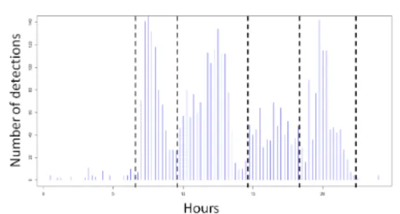
The first idea to model habits is to try to divide a day in several “time slots” based on an activity indicator observed during significant periods of time. Throughout a previous study [11], the number of detection per hour over a 30-days data sample has been chosen as it expresses the presence rate in a room but also the activity (movements within a room and passages between two rooms). Results of this unsupervised classification process (the number of time slots being unknown a priori) are showed in Figure 1.
Figure 1: Time-related classification over 24h during 30 days
65
This time-related classification highlights six distinctive periods concerning the daily home behavior of this person. Light activity is noticed at night, between midnight and 7.30 am and in the evening (with spikes at bedtime), high activity during the morning and the afternoon and medium activity during meal times. For this example, house plan and sensors positions were known. These features are of course unrelated to the installed sensors which give a simple binary indication (presence/no presence). For this particular study, twelve sensors have been used for a total surface
70
of 35m2, enabling a quite precise localization of the person.
An additional characterization step consists in linking an activity to each detection area, that is, in most cases to a specific room of the house. The presence indicator is quantified in presence rate with respect to the total presence in order to normalize data and to manipulate it more easily. We have thus used Telegrafik data to perform this new classification illustrated by Figure 2. It shows the presence rate by room (bedroom, entrance, kitchen, living room)
75
over 24h and a week of observation.
For this person, it can be noticed at first that certain rooms (bedroom, kitchen) have a similar presence profile for each day of the week. Besides, some transitions between two rooms are done t very close hours (for example transition between bedroom and kitchen around 7.30am). Finally, it is possible to distinguish activities such as meal preparation by observing kitchen and living room curves. Thus, the presence rate seems to be a relevant indicator to
80
reflect behavioral habits of a person (these statements being observed in other people). Considering now the number of detections (activities) by adding all detections in each room over a three-weeks period, results for the same person are obtained and illustrated by Figure 3.
Figure 3: Numbre of detection per quarter of an hour over three weeks
Time slots are therefore more visible. Figure 3 shows, with a multi-sensors system, that a day can be divided in 6 time slots. However, three weeks of data are necessary to obtain this division which is quite significant.
85
Time slots determination algorithm
The aim is to compute presence and activity data to obtain an empirical time slots model. The first idea consists in estimating the learning time necessary to see time slots settle down thanks to direct data treatment. For this evaluation, we stacked data over three weeks as illustrated by Figure3.
If we want for example, each day, to tune time slots (duration and beginning/finishing hours), it is difficult to use a
90
sliding window over 21 days. It involves choosing almost fixed time slots (time slots tuning, in case of gradual change of habits, would be too slow).
The approach we chose to use consists in designing a model based on activity and presence, during a learning period of 21 days, according to six time slots, to calculate three indicators:
• Time slot durations,
95
• Start and end hours for each time slot,
• Average level of activity in each time slot.
Once the learning phase is done, each indicator is daily adjusted by weighting the average learned value and the recent new value. Thus daily updates are available and it is possible to rely on regularly updated values to propose a longitudinal monitoring and to compare graphs of the same indicators over several months. Indeed, health
100
practitioners systematically wish to be able to evaluate, in an objective way, effects of their prescriptions between medical check-ups.
With the above considerations, we have applied the following process:
• First, we define a way to divide days in a fixed number of time slots by choosing only one indicator to reduce complexity,
105
• Then, a daily learning procedure of time slots is designed,
• Finally dispersions are observed: indicators’ values stand between minimal and maximal values, also deter-mined during the learning phase.
It is essential to evaluate the sensitivity of the model in order to reach a false alarms level acceptable to people (patient and general practitioner), by tightening or relaxing the minimum and maximum learned values.
110
3. IMPLEMENTATION OF TIME SLOTS DIVISION
In this section, the process is presented step by step and illustrated thanks to equations (all data treatments being coded in R).
3.1. Presence rate indicator
Let∆pres, presence time in room r, at the quarter of an hour 4t ´ q and τprespt, rq, the presence rate at time t, in the
room r. 0 ď∆presp4t ´ q, rq ď 15 min (1) @t P v1, 24w, τprespt, rq “ 100 60 3 ÿ n“0 ∆presp4t ´ q, rq (2)
Bear in mind that it is necessary to take into account the possibility that the person is present but not detected
115
since some rooms are not monitored (toilets, bathroom . . . ). Besides, sensors location may be the origin of errors: the person may be present but not detected by sensors. The algorithm that computes presence takes as input formatted data for the considered day and delivers, as output, presence time for each room and for each quarter of an hour. For each quarter of an hour, two situations can be considered:
• The person is present but inactive: creation of presence at the beginning of the quarter of an hour not detected,
120
in the room where the person has been detected the last time.
• The person is present and the quarter of an hour is already present in data: creation of the next quarter of an hour if it does not exist.
3.2. Time slots calculation
The aim is to determine the “real moments” when a time slot ends. These moments can be defined as “transition
125
points” and are based on simple empirical criteria.
The presence rate has been chosen as the main indicator to perform this division in 6 time slots and to obtain a personalized empirical model. The real-time execution takes place at the end of each day (estimation) and data is included into the learning process. At the beginning, moments of start/end of each time slot Tkare fixed arbitrarily,
then for each time slot, the most used room Rk is identified, and finally the “real moment” of a time slot’s end is
130
estimated (see Table 2).
start end room estimated end T6 1 7 bedroom 7.067168 T1 7 12 kitchen 10.484733 T2 12 14 kitchen 13.495745 T3 14 17 living room 16.494167 T4 17 19 living room 18.998171 T5 19 21 living room 21.918875
Table 2: Estimation of the end and main room for each time slot
A time slot Tkis composed of a theoretical start debk, a theoretical end debk`1and a main room Rk:
@k P v1, K ´ 1w, Tk“ tt|debkă t ă debk`1; Rku (3)
On a one-week sample, main rooms are determined. To do so, presence rate averages are computed depending on rooms and time slots previously fixed.
ˆ
Main room Rkis chosen according to following equation:
ˆ
mk,R“ max
r p ˆmk,rq (5)
After initialization of time slots, they need to be estimated. In other words, a method that evaluates “real moments” corresponding to ends of time slots (transition points) has to be designed. The algorithm determines classes but it is
135
neither a supervised classification (presence data are not assigned to a time slot, that is precisely what we want to do), nor unsupervised classification as the number of classes is known. It is simply based on empirical criteria.
3.2.1. Processing toward functional data
To perform the division, presence rates are processed in order to make them more functional (from an analytical perspective). It means that a function ˆg is determined, that interpolates for each room r points (t ; τprespt, rq). Several
interpolation methods exist (cubic spline, circular, B-spline, polynomial. . . ), but for our study cubic splines have been retained. It constitutes the simplest type of spline to implement, and considering definition of a cubic spline, it is subject to the only constraint we order:
ˆgrptq “ τprespt, rq (6)
The aim is not to predict but only to have a function with which calculations are easily done (derivatives, root(s) calculation. . . ). Let us briefly recall its features. On a particular day and room, n “ 24 couples of (ti; τpresi ) with 140
tiă ti`1called “nodes” and i P 1. . . n ´ 1 are used.
On each interval rti; ti`1s, a 3rd polynomial degree is determined:
@t P rti; ti`1s, ˆgrptq “ aipt ´ tiq3` bipt ´ tiq2` cipt ´ tiq ` di (7)
ˆg is thus twice continuously differentiable on rti; ti`1s (useful to find extrema). This is of little importance for our
issue; the specific feature of natural cubic splines is at the limit of interval.
ˆg2rpt1q “ ˆg2rptnq “ 0 (8)
By using this method to main rooms computed before (except Entrance), we obtained results illustrated by Figure 4.
To identify transitions between time slots, two different criteria have been applied: (1) When the room with the man occupancy rate change between two consecutive time slots, a relevant criterion is to detect “presence reversal”,
145
that is to determine the moment ˆtkclosest to tk(theoretical end of Tk, fixed at initial step) when presence rate in Rk`1
becomes greater than that in Rkbetween the beginning of Tkand the end of Tk`1. Graphically, it merely corresponds
to the point of intersection between the two curves as shown in Figure 4.
Figure 4: Examples of transitions between T6 (bedroom) and T1 (kitchen)
Let ˆgRk, presence function of room Rkand ˆgRk`1presence function of room Rk`1. The set Strof transition points
is obtained by roots calculation of the difference of these two functions. Str“ ttk1 P TkY Tk`1| ˆgRk`1pt 1 kq ´ ˆgRkpt 1 kq “ 0u (9) 6
Roots are computed with R function “uniroot.all” which uses Newton-Raphson numerical method. In this set, the point, for which the absolute difference with the initially fixed end is the smallest, is selected. The estimation of the end of time slot is thus:
ˆtk“ arg t1
kP Str
min | t1
k´ tk| (10)
(2) In the second case, main room remains the same between two consecutive time slots. We wish to split the curve of the considering room in two parts in order to create a temporal frontier ˆtkclosed to tkinitially fixed.
150
The used approach is based on an unsupervised classification algorithm, namely k-medoids algorithm. This al-gorithm is similar to the k-means clustering which determines k means mi for which intra classes dispersions are
minimal considering Euclidean distance. k is arbitrarily chose; in our study we impose k “ 2.
Given a set of observations tx1. . . xnu where each observation is a q-dimensional real vector, class Ciis represented
by its center mi(mean point of the class on the q observation forms):
C “ tC1. . . Ckănu “ argcmin k ÿ i“1 ÿ xjP Ci || xj´ mi||2 (11) mi“ 1 ni ÿ xjP Ci xj (12)
The difference with k-medoid algorithm is that a class is represented by a medoid Mi, that is the point in data
whose average of dissimilarities will all the other points of the class is minimal considering Euclidean distance.
disspx1, x2q “|| x1´ x2||2 (13)
The average dissimilarity of a class Ci is the average distance between all the observations of the class and its
medoid Mi. disspCiq “ 1 ni ÿ xjP Ci || xj´ Mj||2 (14) Mi“ arg xiP tx1...xnu min disspCiq (15)
The determination of classes is done in the same way as for k-means by replacing mipar Miin Eq. 11.
At the first step, the algorithm chooses k randomly points that represent classes. It assigns observations to the
155
closest class. Then it computes classes’ centers. These two last steps are repeated until convergence, i.e. until the value of criterion (Eq. 11) is lower than that of previous step.
K-medoid algorithm is less sensitive to outliers than k-means clustering, but computation time is greater as the computation of medoid takes more time than the one of mean. In our study, it is not an issue because the number of presence data over two time slots (points of interpolated curves) is quite small (around 50 points).
160
Once the two medoids are determined, the average is computed in order to obtain the barycentre of the two classes which corresponds to the estimated moment ˆtk.
ˆtk“
pM1` M2q
2 (16)
An estimated time slot ˆTk,d, during day d, contains thus a start (which is actually the estimation of the end of the previous time slot) and an estimated end.
ˆ
3.3. Time slots deviation
Estimations of time slots remain strongly linked to the presence rate. So, variations of the beginning and/or the end of a slot could imply a change in normal behavior and thus can constitute a second relevant indicator.
First of all, for each slot k, two mean transitions are defined (start= 1 and end = 2) on n “ 3 days, Tk,1,d´1 and Tk,2,d´1for day d ´ 1 based on a sliding mean on ˆTk,1,d´1... ˆTk,1,d´n(Eq. 18).
Tk,1,d´1“ 1 n d´1 ÿ q“d´n ˆ Tk,1,q (18)
Standards deviations associated to Tk,1,d´1and Tk,2,d´1are determined thanks to Eq 19.
σk,1,d´1 “ g f f e 1 n d´1 ÿ q“d´n p ˆTk,1,q´ Tk,1,d´1q2 (19)
Given estimations ˆTk,1,det ˆTk,2,dof a slot, the goal is to design a tolerance interval for both the beginning and the
end of the slot to quantify deviations Dk,1,det Dk,2,dof these estimations with respect to mean and standard deviation
165
at d ´ 1.
In other words, if ˆTk,1,dis within interval rTk,1,d´1´ σk,1,d´1; Tk,1,d´1` σk,1,d´1s, it is not considered as a change of habits. Deviations correspond to the following equation:
Dk,i,d “ ˆ
Tk,i,d´ Tk,i,d´1
2σk,i,d´1 (20)
Tolerance interval for these deviations is thus r´0.5; 0.5s. These deviations are combined by computing the mean total absolute deviation.
Dk,d“| Dk,1,d| ` | Dk,2,d|
2 ˆ 100 (21)
3.4. Learning process implementation
The learning process we designed aims to closely follow the behavior without excessive attenuations or overstate-ments of behavior deviation over time. It will then be used as reference to detect habits changes. The idea is, each time, to learn through simple statistical operators over a fixed-size sliding window. Learned values are annotated with
170
a “˚”. Time slots
Learning process of the end (subscript 2) of a time slot T˚
k,2,d`1 for the following day d ` 1 is based on the
estimation and the learning process of the current day and past according to the following equation:
Tk˚,2,d`1“ Tk,2,d˚ ` λ ˜ ˆ Tk,2,d´1 n d ÿ q“d´n`1 Tk,2,q˚ ¸ (22)
With n the length of the sliding window and λ P s0; 1r. By doing the learning with ground truth data, it appears that the best estimation is obtained with a factor λ between 0.4 and 0.6.
Presence rate
175
The learning of presence rate is done for each time slot where sliding average minima and maxima are computed (considering the main room of the slot). For a slot T˚
k learned, the two following equations are used:
max˚ T˚k,d`1ppresq “ 1 n d ÿ q“d´n`1 max tP T˚k,q τprespt, Rkqq (23) 8
min˚ Tk,d`1˚ ppresq “ 1 n d ÿ q“d´n`1 min tP Tk,q˚ τprespt, Rkqq (24)
Figure 5 shows the obtained results with a sliding window of 4 days over a 21-days period of time. Average of maximum, average of minimum, estimation and sliding average are respectively represented in red, green, black and blue. After ten days of learning, the system is operational as it is possible to monitor in real time deviations of indicators according to the model of the time slot and to determine a first level of detection thanks to a set of rules. For example, a deviation during slot T3 of day 20 can be noticed.
180
Figure 5: Presence learning process over 21 days with a 4-days sliding window for each time slot
Detection of unusual situations
Detection of an unusual presence rate is based on deviation between current presence rate at a given moment t in the main room Rkand learned values for t P Tk,d˚ .
Epτprespt, Rkqq “ max˚ Tk,d˚ppresq ´ τprespt, Rkq max˚ Tk,d˚ppresq ´ min ˚ Tk,d˚ppresq ˆ 100 (25)
Time slot deviation indicator
In the same way as for the presence rate, the learning process for this indicator is done through the use of sliding minimum and maximum average on a window of fixed size n. The equation is however different as only one value of deviation for each slot exists whereas, for presence, several extreme values were used for each slot (calculation of the mean of the n last maximum rates (resp. minimum) in the main room. Here, the mean between maximum deviation (resp. minimum) over the last n days and that learned the day before is computed. By their very nature, the difference between learned presence and time slot deviation, lies in the time scale on which extreme values are computed.
max˚ Tk,d`1˚ pdevq “ max q P rd´n`1;ds Ek,d` max˚ Tk,d˚pdevq 2 (26)
min˚ Tk,d`1˚ pdevq “ min q P rd´n`1;ds Ek,d` min˚ T˚k,dpdevq 2 (27)
For the first n days, all is initialized at 0. Contrary to presence, time slot deviation is not limited, but we decided to reject those greater than 1 during learning. Learned deviation thus falls between 0 and 1, otherwise this could uselessly inflate max˚.
EpDk,dq “ max˚ Tk,d˚pdevq ´ Dk,d max˚ T˚ k,d pdevq ´ min˚ T˚ k,d pdevqˆ 100 (28) 4. Decision-making support
4.1. Design of decision table
The gap will assess the degree of danger of the situation, which will be defined in relation to the value of the gap
185
from threshold s1and another threshold s2. If we consider 3 levels of alert “green”, “orange” and “red”, the decision
might follow the following scheme:
• Red if gap ă 0 or ą s2
• Orange if gap between s1and s2
• Green if gap ă s1
190
The values of the alert thresholds can be first set by the user of the real-time app and adjusted over time if there are too many alerts (this aspect is a perspective point of our work and should ideally be done automatically without human intervention).
The measurement of the deviations from normality on a single indicator has obvious limitations that must be offset by two essential procedures:
195
• The use of several indicators so as to define more precisely the origin of the deviations from normality found,
• The inclusion of the environment and context of the person being supervised: clearly, when a person is subject to ailments, it must be taken into account in the criteria and detection rules of the danger to make a decision on how to proceed.
We advise to work at two different levels of indicator aggregation:
200
• A technical level aiming at ensuring the measurement of the deviation from standard behavior by multiplying the indicators,
• A decision-support level aiming at helping operators assess the danger associated to the alarm according to the person, their surrounding and means of intervention at their disposal.
Thus, these indicators are part of the input from a first detection table and can be combined thanks to easy rules
205
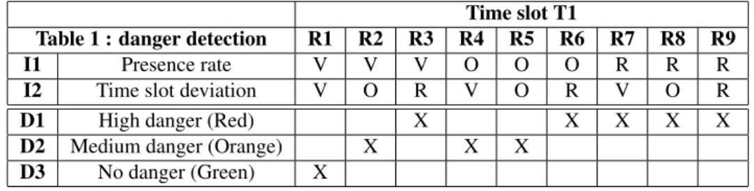
(of the type IF. . . AND IF. . . SO. . . ) so as to establish a first state of alert. For example, an ORANGE presence gap associated to a RED level of deviation will result in a RED degree of danger (see Table 3). This detection is necessary but not sufficient to trigger an intervention, in particuler in case of ORANGE situations. Thus, a second decison table will allow to propose the most relevant and adpated intervention for this personne according to rules defined on the basis of the outputs of the first table , the life context, the person’s profile, its health state...
210
Time slot T1
Table 1 : danger detection R1 R2 R3 R4 R5 R6 R7 R8 R9
I1 Presence rate V V V O O O R R R
I2 Time slot deviation V O R V O R V O R
D1 High danger (Red) X X X X X
D2 Medium danger (Orange) X X X D3 No danger (Green) X
Table 3: Detection table of time slot T1
4.2. Comparative study LAAS/Telegrafik
A first comparative phase was led on two clients of the Telegrafik system for whom they were a few alert occur-rences. We observed good correlation between alarms that prove to be true and launched by Telegrafik system and
215
detections of our system. Indeed, both rooms and time slots were identical (see Table 4).
LAAS Outputs Telegrafik Outputs Room : LIVINGROOM Room : LIVINGROOM
Date : 09/12/2015 Date : 2015-12-09 Presence gap : -21.37 Start of anomaly : 19:22:38 Time slot Deviation gap : 0.784 Alert hour : 22:25:26
Presence level : O Alert : Yes Time slot Deviation level : V Technical problem : No
Danger indicator : presence Time slot : T5
Estimated end of time slot : 23.05
Table 4: Example of LAAS and Telegrafik outputs
The Telegrafik approach lies on a single level based on threshold overrun. The output of the LAAS system is, at the first level, a signal for potential danger based on a color code Green (V) Orange (O) Red (R). Concerning proven
220
alerts, the LAAS system clearly gives at least an orange indicator which should be confirmed by a second level of decision.
As a matter of fact, this detection is necessary but not sufficient to trigger intervention, particularly after orange-type situations. Thus a second decision table will permit, in accordance with rules defined according to the output of the first decision table, the living context, profile of the person and their state of health, to propose the most relevant
225
intervention adapted to this person.
An application named Vigilesoft (Figure 6) was designed and developed so that the end users themselves (supervi-sors, physicians. . . ) can easily configure expert rules for both detection and decision tables. The application’s purpose, once the tables have been configured, is to create simulations using existing data and permit real-time monitoring of the person and a longitudinal follow-up indispensable to physicians to detect slow drifts of behavior. This software
230
platform is completely part of our work on frailty detection of complex systems (man, structure, and environment) and was therefore thought to be independent from the system employed.
5. Conclusion et perspectives
The presence sensor is essential in the monitoring of the elderly at home. It allows to calculate a variable presence rate whose average and real-time values can be at any time compared and used as a basis for the detection of an
235
abnormal situation. The implementation of this concept is nowadays generalized but still delivers unsatisfactory results due to many false alarms.
In this article we are exploring the objective of improving the accuracy of life-style modeling by building a time-slot modeling: each time time-slot is typical of a domestic activity, necessarily reproduced day after day. Thus, we believe we can build more precise and sensitive models allowing to detect situations straying from usual behavior.
Figure 6: Vigilesoft web interface
Using empirical data from several persons, we demonstrate that we might imagine an automatic division into time slots in which the activities are relatively typical and reproducible. In order to exploit this division in a practical way, we assume it static (6 time slots) and calculate, day after day, the begin and end date of the time slot. In this way, we can define several indicators: begin and end date, activity rate within the time slot, presence rate by room within the time slot. We introduce in this article the basis we use to first associate several indicators in a detection
245
table thanks to a set of open rules permitting manual adjustments and an easier understanding of the situation in the field. This detection of a deviation from normality (as it was modelized) is set in the context of a person’s life (case history, surroundings. . . ) so as to obtain the most relevant decision to respond. This was the subject matter of the creation of an application, still currently being developed, which will represent an essential tool in the continuation and enhancement of our work.
250
Our study confirms that measuring presence through low-cost infrared sensors remains an essential path to de-signing home-monitoring systems However this study could be improved. On the one hand, a preliminary phase of cleansing raw motion data seems vital in order to rule out inconsistent data due to environment disruptors (pets, flow of hot air. . . ). On the other hand, thanks to sensor proliferation and optimum positioning for information up-take, the future lies in more detailed and accurate divisions that will provide access to the very nature of the different domestic
255
activities. An even more accurate modeling of normality is possible, that will allow to largely limit the false alarms impairing the mass development of these technologies.
Acknowledgements
The authors of this article wish to thank the Occitanie Region for funding the TELEPASS project (READYNOV program) this work is part of. We equally address thanks to the Telegrafik company for the availability of data and the
260
enriching partnership leading to new thinking and development.
References
[1] Y. Charlon, W. Bourennane, F. Bettahar, E. Campo, Activity monitoring system for elderly in a context of smart home, IRBM 34 (1) (2013) 60–63.
[2] W. Bourennane, Y. Charlon, F. Bettahar, E. Campo, D. Esteve, Homecare monitoring system: A technical proposal for the safety of the elderly
265
experimented in an alzheimer’s care unit, IRBM 34 (2) (2013) 92–100.
[3] P. Barsocchi, M. G. Cimino, E. Ferro, A. Lazzeri, F. Palumbo, G. Vaglini, Monitoring elderly behavior via indoor position-based stigmergy, Pervasive and Mobile Computing 23 (2015) 26–42.
[4] N. Zouba, F. Bremond, M. Thonnat, An activity monitoring system for real elderly at home: Validation study, in: 2010 7th IEEE International Conference on Advanced Video and Signal Based Surveillance, Boston, MA, 2010, pp. 278–285.
270
[5] A. Mitas, M. Rudzki, M. Skotnicka, P. Lubina, Activity monitoring of the elderly for telecare systems - review, Information Technologies in Biomedicine 4 (2014) 125–138.
[6] N. Noury, et al., Monitoring behavior in home using a smart fall sensor and position sensors, in: 1st Annual International IEEE-EMBS Special Topic Conference on Microtechnologies in Medicine and Biology, Lyon, France, 2000, pp. 607–610.
[7] H. Medjahed, D. Istrate, J. Boudy, J. Baldinger, B. Dorizzi, A pervasive multi-sensor data fusion for smart home healthcare monitoring, in:
275
International Conference on Fuzzy Systems (FUZZ-IEEE 2011), Taipei, 2011, pp. 1466–1473.
[8] L. Fried, C. Tangen, J. Walston, A. Newman, C. Hirsch, J. Gottdiener, T. Seeman, R. Tracy, W. Kop, G. Burke, M. McBurnie, Frailty in older adults: evidence for a phenotype, The Journals of Gerontology. Series A, Biological Sciences and Medical Sciences 56 (3) (2001) 146–156. [9] S. Fritz, M. Lusardi, White paper: Walking speed: the sixth vital sign, Journal of Geriatric Physical Therapy 32 (2) (2009) 2–5.
[10] E. Campo, M. Chan, W. Bourennane, D. Est`eve, Behaviour monitoring of the elderly by trajectories analysis, in: 2010 Annual International
280
Conference of the IEEE Engineering in Medicine and Biology, Buenos Aires, 2010, pp. 2230–2233.
[11] S. Bonhomme, E. Campo, D. Est`eve, J. Guennec, Prosafe-extended, a telemedicine platform to contribute to medical diagnosis, Journal of Telemedicine and Telecare 14 (3) (2008) 116–119.