HAL Id: hal-03032262
https://hal.archives-ouvertes.fr/hal-03032262
Submitted on 1 Dec 2020
HAL is a multi-disciplinary open access
archive for the deposit and dissemination of
sci-entific research documents, whether they are
pub-lished or not. The documents may come from
teaching and research institutions in France or
abroad, or from public or private research centers.
L’archive ouverte pluridisciplinaire HAL, est
destinée au dépôt et à la diffusion de documents
scientifiques de niveau recherche, publiés ou non,
émanant des établissements d’enseignement et de
recherche français ou étrangers, des laboratoires
publics ou privés.
Large-scale climate features and climate sensitivity
Alan M. Haywood, Julia C. Tindall, Harry J. Dowsett, Aisling M. Dolan,
Kevin M. Foley, Stephen J. Hunter, Daniel J. Hill, Wing Le Chan, Ayako
Abe-Ouchi, Christian Stepanek, et al.
To cite this version:
Alan M. Haywood, Julia C. Tindall, Harry J. Dowsett, Aisling M. Dolan, Kevin M. Foley, et al.. The
Pliocene Model Intercomparison Project Phase 2: Large-scale climate features and climate sensitivity.
Climate of the Past, European Geosciences Union (EGU), 2020, 16 (6), pp.2095-2123.
�10.5194/cp-16-2095-2020�. �hal-03032262�
https://doi.org/10.5194/cp-16-2095-2020 © Author(s) 2020. This work is distributed under the Creative Commons Attribution 4.0 License.
The Pliocene Model Intercomparison Project Phase 2:
large-scale climate features and climate sensitivity
Alan M. Haywood1, Julia C. Tindall1, Harry J. Dowsett2, Aisling M. Dolan1, Kevin M. Foley2, Stephen J. Hunter1, Daniel J. Hill1, Wing-Le Chan3, Ayako Abe-Ouchi3, Christian Stepanek4, Gerrit Lohmann4, Deepak Chandan5, W. Richard Peltier5, Ning Tan6,7, Camille Contoux7, Gilles Ramstein7, Xiangyu Li8,9, Zhongshi Zhang8,9,10, Chuncheng Guo9, Kerim H. Nisancioglu9, Qiong Zhang11, Qiang Li11, Youichi Kamae12, Mark A. Chandler13, Linda E. Sohl13, Bette L. Otto-Bliesner14, Ran Feng15, Esther C. Brady14, Anna S. von der Heydt16,17,
Michiel L. J. Baatsen17, and Daniel J. Lunt18
1School of Earth and Environment, University of Leeds, Woodhouse Lane, Leeds, West Yorkshire, LS29JT, UK 2Florence Bascom Geoscience Center, U.S. Geological Survey, Reston, VA 20192, USA
3Atmosphere and Ocean Research Institute, The University of Tokyo, Kashiwa, 277-8564, Japan
4Alfred-Wegener-Institut – Helmholtz-Zentrum für Polar and Meeresforschung (AWI), Bremerhaven, 27570, Germany 5Department of Physics, University of Toronto, Toronto, M5S 1A7, Canada
6Key Laboratory of Cenozoic Geology and Environment, Institute of Geology and Geophysics,
Chinese Academy of Sciences, Beijing 100029, China
7Laboratoire des Sciences du Climat et de l’Environnement, LSCE/IPSL, CEA-CNRS-UVSQ,
Université Paris-Saclay, 91191 Gif-sur-Yvette, France
8Institute of Atmospheric Physics, Chinese Academy of Sciences, Beijing 100029, China
9NORCE Norwegian Research Centre, Bjerknes Centre for Climate Research, 5007 Bergen, Norway
10Department of Atmospheric Science, School of Environmental Studies, China University of Geosciences, Wuhan, China 11Department of Physical Geography and Bolin Centre for Climate Research, Stockholm University,
Stockholm, 10691, Sweden
12Faculty of Life and Environmental Sciences, University of Tsukuba, Tsukuba, 305-8572, Japan 13CCSR/GISS, Columbia University, New York, NY 10025, USA
14National Center for Atmospheric Research, (NCAR), Boulder, CO 80305, USA
15Department of Geosciences, College of Liberal Arts and Sciences, University of Connecticut, Storrs, CT 06033, USA 16Centre for Complex Systems Science, Utrecht University, Utrecht, 3584 CS, the Netherlands
17Institute for Marine and Atmospheric research Utrecht (IMAU), Department of Physics,
Utrecht University, Utrecht, 3584 CS, the Netherlands
18School of Geographical Sciences, University of Bristol, Bristol, BS8 1QU, UK
Correspondence:Julia C. Tindall ([email protected])
Received: 29 November 2019 – Discussion started: 2 January 2020
Revised: 24 July 2020 – Accepted: 29 July 2020 – Published: 4 November 2020
Abstract.The Pliocene epoch has great potential to improve our understanding of the long-term climatic and environ-mental consequences of an atmospheric CO2 concentration
near ∼ 400 parts per million by volume. Here we present the large-scale features of Pliocene climate as simulated by a new ensemble of climate models of varying complexity and spatial resolution based on new reconstructions of
bound-ary conditions (the Pliocene Model Intercomparison Project Phase 2; PlioMIP2). As a global annual average, modelled surface air temperatures increase by between 1.7 and 5.2◦C relative to the pre-industrial era with a multi-model mean value of 3.2◦C. Annual mean total precipitation rates in-crease by 7 % (range: 2 %–13 %). On average, surface air temperature (SAT) increases by 4.3◦C over land and 2.8◦C
over the oceans. There is a clear pattern of polar amplifi-cation with warming polewards of 60◦N and 60◦S
exceed-ing the global mean warmexceed-ing by a factor of 2.3. In the At-lantic and Pacific oceans, meridional temperature gradients are reduced, while tropical zonal gradients remain largely unchanged. There is a statistically significant relationship be-tween a model’s climate response associated with a doubling in CO2(equilibrium climate sensitivity; ECS) and its
simu-lated Pliocene surface temperature response. The mean en-semble Earth system response to a doubling of CO2
(includ-ing ice sheet feedbacks) is 67 % greater than ECS; this is larger than the increase of 47 % obtained from the PlioMIP1 ensemble. Proxy-derived estimates of Pliocene sea surface temperatures are used to assess model estimates of ECS and give an ECS range of 2.6–4.8◦C. This result is in general accord with the ECS range presented by previous Intergov-ernmental Panel on Climate Change (IPCC) Assessment Re-ports.
1 Introduction
1.1 Pliocene climate modelling and overview of the Pliocene Model Intercomparison Project
Efforts to understand climate dynamics during the mid-Piacenzian warm period (MP; 3.264 to 3.025 million years ago), previously referred to as the mid-Pliocene warm period, have been ongoing for more than 25 years. This is because the study of the MP enables us to address important scientific questions. The inclusion of a Pliocene experiment within the Coupled Model Intercomparison Project Phase 6 (CMIP6) experimental protocols underlines the general potential of the Pliocene to address questions regarding the long-term sensi-tivity of climate and environments to forcing, as well as the determination of climate sensitivity specifically.
Beginning with the initial climate modelling studies of Chandler et al. (1994), Sloan et al. (1996), and Haywood et al. (2000), the complexity and number of climate models used to study the MP has since increased substantially (e.g. Haywood and Valdes, 2004). This progression culminated in 2008 with the initiation of a co-ordinated international model intercomparison project for the Pliocene (Pliocene Model Intercomparison Project, PlioMIP). PlioMIP Phase 1 (PlioMIP1) proposed a single set of model boundary condi-tions based on the U.S. Geological Survey PRISM3D dataset (Dowsett et al., 2010) and a unified experimental design for atmosphere-only and fully coupled atmosphere–ocean cli-mate models (Haywood et al., 2010, 2011).
PlioMIP1 produced several publications analysing diverse aspects of MP climate. The large-scale temperature and pre-cipitation response of the model ensemble was presented in Haywood et al. (2013a). The global annual mean surface air temperature was found to have increased compared to the pre-industrial era, with models showing warming of between
1.8 and 3.6◦C. The warming was predicted at all latitudes but showed a clear pattern of polar amplification resulting in a reduced Equator to pole surface temperature gradient. Mod-elled sea-ice responses were studied by Howell et al. (2016) who demonstrated a significant decline in Arctic sea-ice ex-tent, with some models simulating a seasonally sea-ice-free Arctic Ocean driving polar amplification of the warming. The reduced meridional temperature gradient influenced atmo-spheric circulation in a number of ways, such as the poleward shift of the middle-latitude westerly winds (Li et al., 2015). In addition, Corvec and Fletcher (2017) studied the effect of reduced meridional temperature gradients on tropical at-mospheric circulation. They demonstrated a weaker tropical circulation during the MP, specifically a weaker Hadley cir-culation, and in some climate models also a weaker Walker circulation, a response akin to model predictions for the fu-ture (IPCC, 2013). Tropical cyclones (TCs) were analysed by Yan et al. (2016) who demonstrated that average global TC intensity and duration increased during the MP, but this result was sensitive to how much tropical sea surface temperatures (SSTs) increased in each model. Zhang et al. (2013, 2016) studied the East Asian and west African summer monsoon response in the PlioMIP1 ensemble and found that both were stronger during the MP, whilst Li et al. (2018) reported that the global land monsoon system during the MP simulated in the PlioMIP1 ensemble generally expanded poleward with increased monsoon precipitation over land.
The modelled response in ocean circulation was also ex-amined in PlioMIP1. The Atlantic Meridional Overturning Circulation (AMOC) was analysed by Zhang et al. (2013). No clear pattern of either weakening or strengthening of the AMOC could be determined from the model ensemble, a re-sult at odds with long-standing interpretations of MP merid-ional SST gradients being a result of enhanced ocean heat transport (OHT; e.g. Dowsett et al., 1992). Hill et al. (2014) analysed the dominant components of MP warming across the PlioMIP1 ensemble using an energy balance analysis. In the tropics, increased temperatures were determined to be predominantly a response to direct CO2forcing, while at
high latitudes, changes in clear sky albedo became the domi-nant contributor, with the warming being only partially offset by cooling driven by cloud albedo changes.
The PlioMIP1 ensemble was used to help constrain equi-librium climate sensitivity (ECS; Hargreaves and Annan, 2016). ECS is defined as the global temperature response to a doubling of CO2once the energy balance has reached
equilibrium (this diagnostic is discussed further in Sect. 2.4). Based on the PRISM3 (Pliocene Research, Interpretation and Synoptic Mapping version 3) compilation of MP tropical SSTs, Hargreaves and Annan (2016) estimated that ECS is between 1.9 and 3.7◦C. In addition, the PlioMIP1 model en-semble was used to estimate Earth system sensitivity (ESS). ESS is defined as the temperature change associated with a doubling of CO2 and includes all ECS feedbacks along
sheets. In PlioMIP1, ESS was estimated to be a factor of 1.47 higher than the ECS (ensemble mean ECS = 3.4◦C;
ensem-ble mean ESS = 5.0◦C; Haywood et al., 2013a).
1.2 From PlioMIP1 to PlioMIP2
The ability of the PlioMIP1 models to reproduce patterns of surface temperature change, reconstructed by marine and ter-restrial proxies, was investigated via data–model compari-son (DMC) in Dowsett et al. (2012, 2013) and Salzmann et al. (2013) respectively. Although the PlioMIP1 ensemble was able to reproduce many of the spatial characteristics of SST and surface air temperature (SAT) warming, the models ap-peared unable to simulate the magnitude of warming recon-structed at the higher latitudes, in particular in the high North Atlantic (Dowsett et al., 2012, 2013; Haywood et al., 2013a; Salzmann et al., 2013). This problem has also been reported as an outcome of DMC studies for other time periods in-cluding the early Eocene (e.g. Lunt et al., 2012). Haywood et al. (2013a, b) discussed the possible contributing factors to the noted discrepancies in DMCs, noting three primary causal groupings: uncertainty in model boundary conditions, uncertainty in the interpretation of proxy data and uncertainty in model physics (for example, recent studies have demon-strated that this model–proxy mismatch has been reduced by including explicit aerosol–cloud interactions in the newer generations of models; Sagoo and Storelvmo, 2017; Feng et al., 2019).
These findings substantially influenced the experimen-tal design for the second phase of PlioMIP (PlioMIP2). Specifically, PlioMIP2 was developed to (a) reduce uncer-tainty in model boundary conditions and (b) reduce un-certainty in proxy data reconstruction. To accomplish (a), state-of-the-art approaches were adopted to generate an en-tirely new palaeogeography (compared to PlioMIP1), includ-ing accountinclud-ing for glacial isostatic adjustments and changes in dynamic topography. This led to specific changes com-pared to the PlioMIP1 palaeogeography capable of influenc-ing climate model simulations (Dowsett et al., 2016; Otto-Bliesner et al., 2017). These include the Bering Strait and Canadian Archipelago becoming subaerial and modifications of the land–sea mask in the Indonesian and Australian re-gion for the emergence of the Sunda and Sahul shelves. To achieve (b), it was necessary to move away from time-averaged global SST reconstructions and towards the exam-ination of a narrow time slice during the late Pliocene that has almost identical astronomical parameters to the present day. This made the orbital parameters specified in model experimental design consistent with the way in which or-bital parameters would have influenced the pattern of sur-face climate and ice sheet configuration preserved in the ge-ological record. Using the astronomical solution of Laskar et al. (2004), Haywood et al. (2013b) identified a suitable inter-glacial event during the late Pliocene (Marine Isotope Stage KM5c, 3.205 Ma). The new PRISM4 (Pliocene Research,
In-terpretation and Synoptic Mapping version 4) community-sourced global dataset of SSTs (Foley and Dowsett, 2019) targets the same interval in order to produce point-based SST data.
Here we briefly present the PlioMIP2 experimental design, details of the climate models included in the ensemble and the boundary conditions used. Following this, we present the large-scale climate features of the PlioMIP2 ensemble fo-cused solely on an examination of the control MP simula-tion designated as a CMIP6 simulasimula-tion (called midPliocene-eoi400) and its differences to simulated conditions for the pre-industrial era (PI). We also present key differences be-tween PlioMIP2 and PlioMIP1. PlioMIP2 sensitivity experi-ments will be presented in subsequent studies. We conclude by presenting the outcomes from a DMC using the PlioMIP2 model ensemble and a newly constructed PRISM4 global compilation of SSTs (Foley and Dowsett, 2019) and by as-sessing the significance of the PlioMIP2 ensemble in under-standing equilibrium climate sensitivity (ECS) and Earth sys-tem sensitivity (ESS).
2 Methods
2.1 Boundary conditions
All model groups participating in PlioMIP2 were required to use standardized boundary condition datasets for the core midPliocene-eoi400 experiment (for wider accessibil-ity, this experiment will hereafter be referred to as PlioCore).
These were derived from the U.S. Geological Survey PRISM dataset, specifically the latest iteration of the reconstruc-tion known as PRISM4 (Dowsett et al., 2016). They include spatially complete gridded datasets at 1◦×1◦ of latitude– longitude resolution for the distribution of land versus sea, topography and bathymetry, as well as vegetation, soils, lakes and land ice cover. Two versions of the PRISM4 bound-ary conditions were produced which are known as enhanced and standard. The enhanced version comprises all PRISM4 boundary conditions including all reconstructed changes to the land–sea mask and ocean bathymetry. However, groups which are unable to change their land–sea mask can use the standard version of the PRISM4 boundary conditions, which provides the best possible realization of Pliocene conditions based around a modern land–sea mask. In practice, all mod-els except MRI-CGCM2.3 were able to utilize the enhanced boundary conditions. For full details of the PRISM4 recon-struction and methods associated with its development, the reader is referred to Dowsett et al. (2016; this special issue).
2.2 Experimental design
The experimental design for PlioCoreand associated PI
con-trol experiments (hereafter referred to as PICtrl) was
pre-sented in Haywood et al. (2016a; this special issue), and the reader is referred to this paper for full details of the
ex-perimental design. In brief, participating model groups had a choice of which version of the PRISM4 boundary condi-tions to implement (standard or enhanced). This approach was taken in recognition of the technical complexity as-sociated with the modification of the land–sea mask and ocean bathymetry in some of the very latest climate and earth system models. A choice was also included regard-ing the treatment of vegetation. Model groups could either prescribe vegetation cover from the PRISM4 dataset (vege-tation sourced from Salzmann et al., 2008) or simulate the vegetation using a dynamic global vegetation model. If the latter was chosen, all models were required to be initialized with pre-industrial vegetation and spun up until an equilib-rium vegetation distribution was reached. The concentration of atmospheric CO2for experiment PlioCore was set at 400
parts per million by volume (ppmv), a value almost iden-tical to that chosen for the PlioMIP1 experimental design (405 ppmv) and in line with the very latest high-resolution proxy reconstruction of atmospheric CO2of ∼ 400 ppmv for
∼3.2 million years ago using boron isotopes (De La Vega et al., 2018). However, we acknowledge that there are un-certainties on the KM5c CO2value; hence, the specification
of Tier 1 PlioMIP2 experiments (Haywood et al., 2016a), which have CO2 of ∼ 350 and 450 ppmv, will be used to
investigate CO2 uncertainty at a later date. All other trace
gases, orbital parameters and the solar constant were spec-ified to be consistent with each model’s PICtrl experiment.
The Greenland Ice Sheet (GIS) was confined to high eleva-tions in the eastern Greenland mountains, covering an area approximately 25 % of the present-day GIS. The PlioMIP2 Antarctic ice sheet configuration is the same as PlioMIP1 and has no ice over western Antarctica. The reconstructed PRISM4 ice sheets have a total volume of 20.1 × 10⁶km3, which is equal to a sea-level increase relative to the present day of less than ∼ 24 m (Dowsett et al., 2016; this special issue). The integration length was set to be as long as pos-sible or a minimum of 500 simulated years; however, all but two of the modelling groups in PlioMIP2 contributed simulations that were in excess of 1000 years (Table S1 in the Supplement). All modelling groups were requested to fully detail their implementation of PRISM4 boundary con-ditions along with the initialization and spin-up of their ex-periments in separate dedicated papers that also present some of the key scientific results from each model or family of models (see the separate papers within this special volume: https://cp.copernicus.org/articles/special_issue642.html, last access: 16 September 2020, Haywood et al., 2016b). NetCDF versions of all boundary conditions used for the PlioCore
ex-periment, along with guidance notes for modelling groups, can be found here: https://geology.er.usgs.gov/egpsc/prism/ 7.2_pliomip2_data.html (last access: 16 September 2020).
2.3 Participating models
There are currently 16 climate models that have completed the PlioCore experiment to comprise the PlioMIP2
ensem-ble. These models were developed at different times and have differing levels of complexity and spatial resolution. A further model HadGEM3 is currently running the PlioCore
experiment and results from this model will be compared with the rest of the PlioMIP2 ensemble in a subsequent paper. The current 16 model ensemble is double the size of the coupled atmosphere–ocean ensemble presented in the PlioMIP1 large-scale features publication (Haywood et al., 2013a). Summary details of the included models and model physics, along with information regarding the imple-mentation of PRISM4 boundary conditions and each model’s ECS, can be found in Tables 1 and S1. Each modelling group uploaded the final 100 years of each simulation for analysis. These were then regridded onto a regular 1◦×1◦grid using a bilinear interpolation to enable each model to be analysed in the same way. Means and standard deviations for each model were then calculated across the final 50 years.
2.4 Equilibrium climate sensitivity (ECS) and Earth system sensitivity (ESS)
In Sect. 3.6, we use the PlioCoreand PICtrlsimulations to
in-vestigate ECS and ESS. The PlioCore experiments represent
a 400 ppmv world that is in quasi-equilibrium with respect to both climate and ice sheets and hence represents an “Earth system” response to the 400 ppmv CO2 forcing. The Earth
system response to a doubling of CO2 (i.e. 560–280 ppmv;
ESS) can then be estimated as follows:
ESS =ln
560 280
ln400280(PlioCore[SAT] − PICtrl[SAT]) . (1) There will be errors in the estimate of ESS from the above equation; for example, the equation assumes that the sen-sitivity to CO2 is linear, which may not necessarily be the
case. Further errors will occur because of changes between PlioCore and PICtrl which should not be included in
esti-mates of ESS, such as land–sea mask changes, topographic changes, changes in soil properties and lake changes. How-ever, all these additional changes are likely minimal com-pared to the ice sheet and greenhouse gas (GHG) changes and are expected to have only a negligible impact on the glob-ally averaged temperature and therefore the estimate of ESS. For example, Pound et al. (2014) found that the inclusion of Pliocene soils and lake distributions in a climate model had an insignificant effect on global temperature (even though changes regionally could be important).
To assess the relationship across the ensemble between the reported ECS and the modelled ESS, we correlate reported ECS across the ensemble with the associated PlioCore–PICtrl
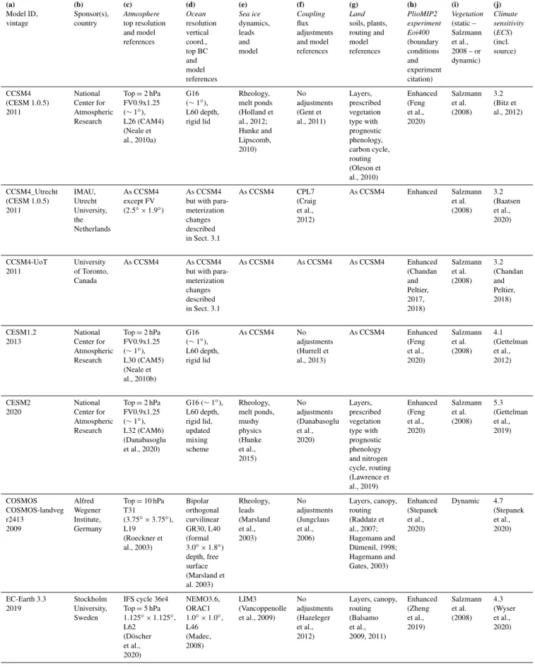
Table 1.Details of climate models used with the PlioCoreexperiment (a–g) plus details of boundary conditions (h), treatment of vegetation (i)
and equilibrium climate sensitivity values (j) (◦C).
(a) (b) (c) (d) (e) (f) (g) (h) (i) (j)
Model ID, Sponsor(s), Atmosphere Ocean Sea ice Coupling Land PlioMIP2 Vegetation Climate vintage country top resolution resolution dynamics, flux soils, plants, experiment (static – sensitivity
and model vertical leads adjustments routing and Eoi400 Salzmann (ECS) references coord., and and model model (boundary et al., (incl.
top BC model references references conditions 2008 – or source)
and and dynamic)
model experiment
references citation)
CCSM4 National Top = 2 hPa G16 Rheology, No Layers, Enhanced Salzmann 3.2 (CESM 1.0.5) Center for FV0.9x1.25 (∼ 1◦), melt ponds adjustments prescribed (Feng et al. (Bitz et
2011 Atmospheric (∼ 1◦), L60 depth, (Holland et (Gent et vegetation et al., (2008) al., 2012)
Research L26 (CAM4) rigid lid al., 2012; al., 2011) type with 2020) (Neale et Hunke and prognostic
al., 2010a) Lipscomb, phenology, 2010) carbon cycle,
routing (Oleson et al., 2010)
CCSM4_Utrecht IMAU, As CCSM4 As CCSM4 As CCSM4 CPL7 As CCSM4 Enhanced Salzmann 3.2 (CESM 1.0.5) Utrecht except FV but with para- (Craig et al. (Baatsen 2011 University, (2.5◦×1.9◦) meterization et al., (2008) et al.,
the changes 2012) 2020)
Netherlands described in Sect. 3.1
CCSM4-UoT University As CCSM4 As CCSM4 As CCSM4 As CCSM4 As CCSM4 Enhanced Salzmann 3.2 2011 of Toronto, but with para- (Chandan et al. (Chandan
Canada meterization and (2008) and
changes Peltier, Peltier,
described 2017, 2018)
in Sect. 3.1 2018)
CESM1.2 National Top = 2 hPa G16 As CCSM4 No As CCSM4 Enhanced Salzmann 4.1 2013 Center for FV0.9x1.25 (∼ 1◦), adjustments (Feng et al. (Gettelman
Atmospheric (∼ 1◦), L60 depth, (Hurrell et et al., (2008) et al.,
Research L30 (CAM5) rigid lid al., 2013) 2020) 2012) (Neale et
al., 2010b)
CESM2 National Top = 2 hPa G16 (∼ 1◦), Rheology, No Layers, Enhanced Salzmann 5.3 2020 Center for FV0.9x1.25 L60 depth, melt ponds, adjustments prescribed (Feng et al. (Gettelman
Atmospheric (∼ 1◦), rigid lid, mushy (Danabasoglu vegetation et al., (2008) et al.,
Research L32 (CAM6) updated physics et al., type with 2020) 2019) (Danabasoglu mixing (Hunke 2020) prognostic
et al., 2020) scheme et al., phenology 2015) and nitrogen
cycle, routing (Lawrence et al., 2019)
COSMOS Alfred Top = 10 hPa Bipolar Rheology, No Layers, canopy, Enhanced Dynamic 4.7 COSMOS-landveg Wegener T31 orthogonal leads adjustments routing (Stepanek (Stepanek r2413 Institute, (3.75◦×3.75◦), curvilinear (Marsland (Jungclaus (Raddatz et et al., et al.,
2009 Germany L19 GR30, L40 et al., et al., al., 2007; 2020) 2020) (Roeckner et (formal 2003) 2006) Hagemann and
al., 2003) 3.0◦×1.8◦) Dümenil, 1998; depth, free Hagemann and surface Gates, 2003) (Marsland et
al. 2003)
EC-Earth 3.3 Stockholm IFS cycle 36r4 NEMO3.6, LIM3 No Layers, canopy, Enhanced Salzmann 4.3 2019 University, Top = 5 hPa ORAC1 (Vancoppenolle adjustments routing (Zheng et al. (Wyser
Sweden 1.125◦×1.125◦, 1.0◦×1.0◦, et al., 2009) (Hazeleger (Balsamo et al., (2008) et al., L62 L46 et al., et al., 2019) 2020) (Döscher (Madec, 2012) 2009, 2011)
et al., 2008) 2020)
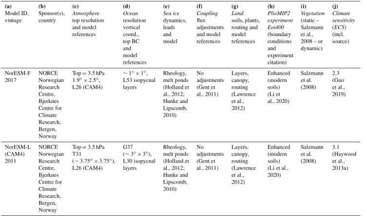
Table 1.Continued.
(a) (b) (c) (d) (e) (f) (g) (h) (i) (j)
Model ID, Sponsor(s), Atmosphere Ocean Sea ice Coupling Land PlioMIP2 Vegetation Climate vintage country top resolution resolution dynamics, flux soils, plants, experiment (static – sensitivity
and model vertical leads adjustments routing and Eoi400 Salzmann (ECS) references coord., and and model model (boundary et al., (incl.
top BC model references references conditions 2008 – or source)
and and dynamic)
model experiment
references citation)
GISS2.1G Goddard Top = 0.1 mb 1.0◦×1.25◦, Visco-plastic No Layers, Enhanced Salzmann 3.3
2019 Institute 2.0◦×2.5◦, P∗, rheology, adjustments canopy, et al. (Kelley
for Space L40 free surface leads, (Kelley et routing (2008) et al., Studies, (Kelley et (Kelley et melt ponds al., 2020) (Kelley 2020) USA al., 2020) al., 2020) (Kelley et et al.,
al., 2020) 2020)
HadCM3 University Top = 5 hPa 1.25◦×1.25◦, Free drift, No Layers, Enhanced Salzmann 3.5 1997 of Leeds, 2.5◦×3.75◦, L20 leads adjustments canopy, (Hunter et al. (Hunter
United L19 depth, (Cattle and (Gordon routing et al., (2008) et al., Kingdom (Pope et rigid lid Crossley, et al., (Cox et 2019) 2019)
al., 2000) (Gordon et 1995) 2000) al., 1999) al., 2000)
IPSLCM6A-LR Laboratoire Top = 1 hPa 1◦×1◦, Thermodynamics, No Layers, Enhanced Salzmann 4.8
2018 des Sciences 2.5◦×1.26◦, refined at 1/3◦ rheology, adjustments canopy, (Lurton et al. (Boucher
du Climat et L79 in the tropics, leads (Marti et routing, et al., (2008) et al., de l’Environnement (Hourdin L75 (Vancoppenolle al., 2010; phenology 2020) 2020) (LSCE), France et al., free surface, et al., 2009; Boucher et (Boucher
2020) zcoordinates Rousset et al., 2020) et al., (Madec et al., 2015) 2020) al., 2017)
IPSLCM5A2.1 LSCE Top = 70 km 0.5◦–2◦×2◦, Thermodynamics, No Layers, Enhanced Salzmann 3.6
2017 France 3.75◦×1.9◦, L31 rheology, adjustments canopy, (Tan et al. (Pierre
L39 free surface, leads (Marti et routing, et al., (2008) Sepulchre, (Hourdin et al., zcoordinates (Fichefet and al., 2010; phenology 2020) personal 2006, 2013; (Dufresne et Morales-Maqueda, Sepulchre (Krinner et communi-Sepulchre et al., 2013; 1997, 1999; et al., al., 2005; cation, al., 2020) Madec et Sepulchre 2020) Marti et 2019)
al., 1996; et al., al., 2010; Sepulchre et 2020) Dufresne et
al., 2020) al., 2013)
IPSLCM5A LSCE Top = 70 km 0.5◦–2◦×2◦, Thermodynamics, No Layers, Enhanced Salzmann 4.1 2010 France 3.75◦×1.9◦, L31 rheology, adjustments canopy, (Tan et al. (Dufresne
L39 free surface, leads (Marti et routing, et al., (2008) et al., (Hourdin zcoordinates (Fichefet and al., 2010; phenology 2020) 2013) et al., (Dufresne et Morales-Maqueda, Dufresne (Krinner et
2006, 2013) al,. 2013; 1997, 1999) et al., al., 2005; Madec et 2013) Marti et
al., 1996) al., 2010;
Dufresne et al., 2013)
MIROC4m Center for Climate Top = 30 km 0.5◦–1.4◦×1.4◦, Rheology, leads No Layers, Enhanced Salzmann 3.9
2004 System Research T42 L43 (K-1 Develo- adjustments canopy, (Chan and et al. (Uploaded (Uni. Tokyo, (∼ 2.8◦×2.8◦) sigma/depth pers, 2004) (K-1 Develo- routing Abe-Ouchi, (2008) 2 × CO
2
National Inst. L20 free surface pers, 2004) (K-1 Develo- 2020) minus PI for Env. Studies, (K-1 model developers, (K-1 Developers, pers, 2004; experiment) Frontier Research 2004) 2004) Oki and Sud,
Center for 1998)
Global Change, JAMSTEC), Japan
MRI-CGCM 2.3 Meteorological Top = 0.4 hPa 0.5◦–2.0◦×2.5◦, Free drift, Heat, fresh Layers, Standard Salzmann 2.8
2006 Research T42 L23 leads water and canopy, (Kamae et al. (Uploaded Institute and (∼ 2.8◦×2.8◦) depth, (Mellor and momentum routing et al., (2008) 2 × CO
2
University of L30 rigid lid Kantha, (12◦S–12◦N) (Sellers 2016) minus PI
Tsukuba, (Yukimoto (Yukimoto 1989) (Yukimoto et al., experiment)
Japan et al., et al., et al., 1986;
2006) 2006) 2006) Sato et
Table 1.Continued.
(a) (b) (c) (d) (e) (f) (g) (h) (i) (j)
Model ID, Sponsor(s), Atmosphere Ocean Sea ice Coupling Land PlioMIP2 Vegetation Climate vintage country top resolution resolution dynamics, flux soils, plants, experiment (static – sensitivity
and model vertical leads adjustments routing and Eoi400 Salzmann (ECS) references coord., and and model model (boundary et al., (incl.
top BC model references references conditions 2008 – or source)
and and dynamic)
model experiment
references citation)
NorESM-F NORCE Top = 3.5 hPa ∼1◦×1◦, Rheology, No Layers, Enhanced Salzmann 2.3 2017 Norwegian 1.9◦×2.5◦, L53 isopycnal melt ponds adjustments canopy, (modern et al. (Guo
Research L26 (CAM4) layers (Holland et (Gent et routing soils) (2008) et al., Centre, al., 2012; al., 2011) (Lawrence (Li et 2019) Bjerknes Hunke and et al., al., 2020)
Centre for Lipscomb, 2012)
Climate 2010)
Research, Bergen, Norway
NorESM-L NORCE Top = 3.5 hPa G37 Rheology, No Layers, Enhanced Salzmann 3.1 (CAM4) Norwegian T31 (∼ 3◦×3◦), melt ponds adjustments canopy, (modern et al. (Haywood 2011 Research (∼ 3.75◦×3.75◦), L30 isopycnal (Holland et (Gent et routing soils) (2008) et al.,
Centre, L26 (CAM4) layers al., 2012; al., 2011) (Lawrence (Li et al., 2013a)
Bjerknes Hunke and et al., 2020)
Centre for Lipscomb, 2012)
Climate 2010)
Research, Bergen, Norway
and local scales. A strong correlation at a particular loca-tion would suggest that MP proxy data at that localoca-tion could be used to derive proxy-data-constrained estimate of ECS (similar to an emergent constraint), while a weak correlation would suggest that proxy data at that location could not be used in ECS estimates.
3 Climate results
3.1 Surface air temperature (SAT)
Figure 1a shows the global mean surface air temperature (SAT) for each model. The top panel shows the PlioCore
and PICtrlSATs, while the lower panel shows the anomaly
between them. In this and all subsequent figures, the mod-els are ordered by ECS (see Table 2) such that the model with the highest published ECS (i.e. CESM2; ECS = 5.3) is shown on the left, while the model with the lowest pub-lished ECS (i.e. NorESM1-F; ECS = 2.3) is on the right. Increases in PlioCore global annual mean SATs, compared
to each of the contributing models PICtrlexperiment, range
from 1.7 to 5.2◦C (Fig. 1a; Table 2) with an ensemble mean 1T of 3.2◦C. The multi-model median 1T is 3.0◦C, while the 10th and 90th percentiles are 2.1 and 4.8◦C re-spectively. Analogous results from individual models of the PlioMIP1 ensemble are shown by the horizontal grey lines in Fig. 1a and have a mean warming of 2.7◦C. Pliocene
warm-ing for individual PlioMIP1 models falls into two distinct anomaly bands that are 1.8–2.2◦C (CCSM4, GISS-E2-R, IP-SLCM5A, MRI2.2) and 3.2–3.6◦C (COSMOS, HadCM3,
MIROC4m, NorESM-L). PlioMIP2 shows a greater range of responses than PlioMIP1, and PlioMIP2 results are more evenly scattered over the ensemble range. The ensemble mean temperature anomaly is larger in PlioMIP2 than in PlioMIP1 because of the addition of new and more sensi-tive models to PlioMIP2 rather than being due to the change in boundary conditions between PlioMIP1 and PlioMIP2.
PlioMIP2 shows increased SATs over the whole globe (Fig. 1b) with an ensemble average warming of ∼ 2.0◦C for the tropical oceans (20◦N–20◦S), which increases towards the high latitudes (Fig. 1b, c). Multi-model mean SAT warm-ing can exceed 12◦C in Baffin Bay and 7◦C in the Green-land Sea (Fig. 1b), a result potentially influenced by the clo-sure of the Canadian Archipelago and Bering Strait, as well as by the specified loss of most of the Greenland Ice Sheet (GIS) and the simulated reduction in Northern Hemisphere sea-ice cover (de Nooijer et al., 2020). In the Southern Hemi-sphere, warming is pronounced in regions of Antarctica that were deglaciated in the MP in both west and east Antarctica (Fig. 1b). Warming in the interior of east Antarctica is lim-ited by the prescribed topography of the MP East Antarctic Ice Sheet (EAIS), which in some places exceeds the topog-raphy of the EAIS in the models’ PICtrlexperiments.
Figure 1.(a) Global mean near-surface air temperature (SAT) for the PlioCoreand PICtrlexperiments from each PlioMIP2 model (upper
panel) and the difference between them (PlioCore–PICtrl) (lower panel). Crosses show the mean value, while the vertical bars show the
inter-annual standard deviation. Horizontal grey lines on the lower panel show the anomalies from individual PlioMIP1 models. (b) Multi-model mean PlioCore–PICtrlSAT anomaly. (c) Latitudinal mean PlioCore–PICtrlSAT anomaly from each PlioMIP2 model. The PlioMIP2
multi-model mean is shown by the dashed black line. The grey shaded area shows the range of values of the PlioMIP1 multi-models. The PlioMIP1 multi-model mean is shown by the dotted black line. (d) Intermodel standard deviation for the PlioCore–PICtrlanomaly.
In terms of magnitude, the CESM2 model has the great-est apparent sensitivity to imposing MP boundary conditions with a simulated 1T of 5.2◦C (Fig. 1a). This model was
pub-lished in 2020 and has the highest ECS of all the PlioMIP2 models. This model was not included in PlioMIP1, and its response to Pliocene boundary conditions lies outside the range of all PlioMIP1 models both in global mean and for every latitude band (Fig. 1a, c). It is also warmer than the PlioMIP2 multi-model mean in nearly all grid boxes (Fig. S1 in the Supplement). Other particularly sensitive models (EC-Earth3.3, CESM1.2, CCSM4-Utr and CCSM4-UoT; shown as an anomaly from the multi-model mean in Fig. S1) are also new to PlioMIP2, and this explains why the simulated 1T from PlioMIP2 exceeds that from PlioMIP1. The model with the lowest response to PlioMIP2 boundary conditions
is the NorESM1-F model, which is also the model with the lowest published ECS. Although there is clearly some cor-relation between a model’s ECS and its PlioCore–PICtl
tem-perature anomaly, the relationship is not exact. In particular, the versions of CCSM4 that were run by Utrecht University (CCSM4-Utr) and the University of Toronto (CCSM-UoT) both show a large Pliocene response but have a modest ECS compared to the other models.
Three different versions of CCSM4 contributed to PlioMIP2 (see Table 1): the standard version run at the Na-tional Center for Atmospheric Research (NCAR) (hereafter referred to as CCSM) has a simulated 1T = 2.6◦C, while CCSM4-Utr has a simulated 1T = 4.7◦C, and CCSM4-UoT has a simulated 1T = 3.8◦C. A notable difference be-tween these simulations is the response in the 60–90◦S band
Table 2.Details of the relationship between the equilibrium climate sensitivity (ECS) and the Earth system sensitivity (ESS) for each model. MMM denotes the multi-model mean.
Model name ECS Eoi400 E280 Eoi400-E280 ESS ESS/CS SAT SAT SAT (Eq. 1) ratio CCSM4-Utrecht 3.2 18.9 13.8 4.7 9.1 2.85 CCSM4 3.2 16.0 13.4 2.6 5.1 1.59 CCSM4-UoT 3.2 16.8 13.0 3.8 7.3 2.29 CESM1.2 4.1 17.3 13.3 4.0 7.7 1.89 CESM2 5.3 19.3 14.1 5.2 10.0 1.88 COSMOS 4.7 16.9 13.5 3.4 6.5 1.39 EC-Earth3.3 4.3 18.2 13.3 4.8 9.4 2.18 GISS2.1G 3.3 15.9 13.8 2.1 4.0 1.22 HadCM3 3.5 16.9 14.0 2.9 5.6 1.60 IPSLCM6A 4.8 16.0 12.6 3.4 6.5 1.36 IPSLCM5A2 3.6 15.3 13.2 2.2 4.2 1.17 IPSLCM5A 4.1 14.4 12.1 2.3 4.5 1.11 MIROC4m 3.9 15.9 12.8 3.1 6.0 1.54 MRI-CGCM2.3 2.8 15.1 12.7 2.4 4.7 1.66 NorESM-L 3.1 14.6 12.5 2.1 4.1 1.33 NorESM1-F 2.3 16.2 14.5 1.7 3.3 1.45 MMM 3.7 16.5 13.3 3.2 6.2 1.67
where the mean warming in the CCSM4-Utr simulation is 4◦C higher than in the CCSM4-UoT simulation and 6.6◦C higher than in the CCSM4 simulation (Figs. 1c, S1). Table S1 shows that, even though the CCSM4 models differ in their response, they all appear to be close to equilibrium. In ad-dition, they are all reported to have similar ECSs (Table 1), and they all have the same physics apart from changes to the standard ocean model in the CCSM4-UoT simulations and the PlioCoreCCSM4-Utr simulation. These changes
(dis-cussed by Chandan and Peltier, 2017, this special issue) are as follows: (1) the vertical profile of background diapycnal mixing has been fixed to a hyperbolic tangent form, and (2) tidal mixing and dense water overflow parameterization schemes have been turned off. Although the exact cause of the differences in 1T between the CCSM4 models remains unclear, the changes in the ocean parameterizations and dif-ferences in initialization may contribute to the 1T differ-ences, in particular the changes in ocean mixing between dif-ferent versions of the model (Fedorov et al., 2010).
Analysis of the standard deviation of the model ensem-ble (Fig. 1d) indicates that models are generally consistent in terms of the magnitude of temperature response in the tropics, especially over the oceans. However, they can dif-fer markedly in the higher latitudes where the inter-model standard deviation reaches more than 4.5◦C.
To evaluate whether the multi-model mean PlioCore–PICtrl
anomaly at a grid box is “robust” we follow the methodology of Mba et al. (2018) and Nikulin et al. (2018). The anomaly is said to be robust if two conditions are fulfilled: (1) at least 80 % models agree on the sign of the anomaly, and (2) the signal-to-noise ratio (i.e. the ratio of the size of the mean anomaly to the inter-model standard deviation; Fig. 1b, d) is
Figure 2.PlioCore–PICtrl SAT multi-model mean anomaly. Grid
boxes where at least 80 % of the models agree on the sign of the change are marked “/”. Grid boxes where the ratio of the multi-model mean SAT change to the PICtrl intermodel standard devia-tion is greater than 1 are marked “\”. Grid boxes where both these conditions are satisfied show a robust signal.
greater than or equal to 1. Regions where the SAT anomaly is considered robust according to these criteria are hatched in Fig. 2. It is seen that for SAT the PlioCore–PICtrlanomaly
is considered robust across the ensemble over nearly all the globe.
3.2 Seasonal cycle of surface air temperature, land–sea temperature contrasts and polar amplification
The Northern Hemisphere (NH) averaged SAT anomaly over the seasonal cycle is presented in Fig. 3a. Overall, the en-semble mean anomaly (dashed black line) is fairly constant throughout the year; however, models within the ensemble have very different characteristics in terms of the monthly and seasonal distribution of the warming. Some members of the ensemble have a relatively flat seasonal cycle in 1SAT (e.g. NorESM-L, NorESM1-F, COSMOS); however, others show a very strong seasonal cycle. The models that show a very strong seasonal cycle do not agree on the timing of the peak warming. For example, EC-Earth3.3 has the peak warming in October, CESM2 has peak warming in July, and MRI2.3 has peak warming in January/February. The lack of consistency in the seasonal signal of warming has in-teresting implications in terms of whether PlioMIP2 out-puts could be used to examine the potential for seasonal bias in proxy datasets. To do this meaningfully would re-quire clear consistency in model seasonal responses, which is absent in the PlioMIP2 ensemble. The grey shaded area in Fig. 3a shows the range of NH temperature responses in PlioMIP1, with the PlioMIP1 ensemble average shown by the dotted black line. Although the ensemble average from both PlioMIP2 and PlioMIP1 shows a relatively flat seasonal cycle, the range of responses is very different between the two ensembles. PlioMIP1 predicted a large range of tem-perature responses in the NH winter, which reduced in the summer. In PlioMIP2, however, the summer range is ampli-fied compared to the winter. Indeed 7 of the 16 PlioMIP2 models show a NH summer temperature anomaly that is no-ticeably above that seen in any of the PlioMIP1 simulations. Some of these models (CESM2, EC-Earth3.3, CCSM4-Utr, CCSM4-UoT and CESM1.2) did not contribute to PlioMIP1, which shows that whichever models are included in an en-semble can strongly affect the enen-semble response. However, other models (MIROC4m and HadCM3) that show an en-hanced summer response in PlioMIP2 were also included in PlioMIP1, showing that there is also an impact of the change in boundary conditions on seasonal temperature. None of the PlioMIP2 models replicate the lowest warming seen in December–February (DJF) in the PlioMIP1 ensemble; this lowest value was derived from the GISS-E2-R model in PlioMIP1 which did not contribute to PlioMIP2.
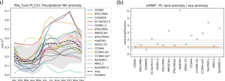
The ensemble results for land–sea temperature contrasts clearly indicate a greater warming over land than over the oceans (Fig. 3b). This result also holds when only the land– sea temperature contrast in the tropics is considered. The land amplification factor is similar in PlioMIP2 and PlioMIP1, and models in both ensembles cluster near a land amplifica-tion factor of ∼ 1.5. There is also no relaamplifica-tionship between a model’s climate sensitivity and the land amplification factor. The multi-model median (10th percentile/90th percentile)
warming over the land and ocean is 4.5◦C (2.6◦C/6.1◦C) and 2.5◦C (1.9◦C/4.4◦C) respectively.
The extratropical NH (45–90◦N) warms more than the
ex-tratropical Southern Hemisphere (SH) (45–90◦S) in 5 of the 8 models (62 %) from PlioMIP1 and in 11 of the 16 mod-els (69 %) from PlioMIP2 (Fig. 3c). This shows that neither the change in boundary conditions nor the addition of newer models to PlioMIP2 affects the ensemble proportion of en-hanced NH warming; nor does the published ECS have any obvious impact on whether the warming is concentrated in the NH or the SH. The models that indicate greater SH ver-sus NH warming (CCSM4-Utr, GISS2.1G, NorESM-L) are among those that have weaker differences between land and ocean warming (Fig. 3b).
Polar amplification (PA) can be defined as the ratio of po-lar warming (poleward of 60◦in each hemisphere) to global mean warming (Smith et al., 2019). The PA for each model for the NH and the SH is shown in Fig. 3d. All models show PA > 1 for both hemispheres, although whether there is more PA in the NH or SH is a model-dependent fea-ture. The ensemble mean (median) PA is 2.3 (2.2) in both the NH and the SH, suggesting that across the ensemble PA is hemispherically symmetrical. This result is very sim-ilar to PlioMIP1 (not shown), which suggests that the en-hanced warming in the PlioMIP2 ensemble does not affect the PA. For PlioMIP2, the NH median PA is 2.2 with the 10th and 90th percentiles at 1.9 and 2.8 respectively, while in the SH the median PA is 2.2, with the 10th and 90th per-centiles at 1.8 and 3.1 respectively. Polar amplification is lower over the land than the ocean (Fig. S2) in both hemi-spheres. The NH mean (10th / 50th / 90th percentiles) PAs are 1.6 (1.4/1.6/1.9) and 2.7 (2.4/2.7/3.3) over the land and ocean respectively, while the SH mean (10th / 50th / 90th percentiles) PAs are 0.9 (0.5/0.8/1.5) and 1.9 (1.1/1.9/2.5) over the land and ocean respectively. Note that in the SH to-tal PA is higher than both land and ocean PAs because of the change in the area of land between the PlioCoreand PICntl
ex-periments. There appears to be a weak relationship between the PA factor and a model’s ECS. Those models which have a lower published ECS (those to the right of Fig. 3d) have a tendency towards a higher PA. This is not because these mod-els have excess warming at high latitudes, but rather these models have less tropical warming than other models.
3.3 Meridional/zonal SST gradients in the Pacific and Atlantic
There has been great interest in the reconstruction of Pliocene SST gradients in the Atlantic and Pacific to pro-vide first order assessments of Pliocene climate change and to assess possible mechanisms of Pliocene temperature en-hancement and ocean–atmospheric dynamic responses (Rind and Chandler, 1991). For example, the meridional gradient in the Atlantic has been discussed in terms of the potential for enhanced ocean heat transport in the Pliocene (e.g. Dowsett
Figure 3.(a) Monthly mean NH PlioCore–PICtrlSAT anomaly for each PlioMIP2 model, with the PlioMIP2 multi-model mean shown by
the dashed black line. The grey shaded region shows the range of values simulated by the PlioMIP1 models, and the PlioMIP1 multi-model mean is shown by the dotted black line. (b) SAT anomaly for land (blue) and sea (orange) from each model averaged over the globe (top panel) and the 20◦N–20◦S region (lower panel). (c) SAT anomaly for the northern extratropics (blue) and southern extratropics (orange) (top panel) and the ratio between them (lower panel). The horizontal grey lines on the lower panel show the values from individual PlioMIP1 models. (d) SAT anomaly poleward of 60◦divided by the globally averaged SAT anomaly for the NH (blue) and the SH (orange). The red line highlights a ratio of 1 (i.e. no polar amplification).
et al., 1992). In addition, the zonal SST gradient across the tropical Pacific has been used to examine the potential for change in Walker Circulation and, through this, El Niño– Southern Oscillation (ENSO) dynamics and teleconnection patterns during the Pliocene (Fedorov et al., 2013; Burls and Fedorov, 2014; Tierney et al., 2019).
The multi-model mean meridional profile of zonal mean SSTs in the Atlantic Ocean is shown in Fig. 4a. In the trop-ics and subtroptrop-ics, the SST increase between the PlioCoreand
PICtrlexperiments is 1.5–2.5◦C. This difference increases to
∼5.0◦C in the NH at ∼ 55◦N with an inter-model range
of 2–11◦C. The Pliocene and pre-industrial meridional SST
profile in the Pacific (Fig. 4b) is similar to that of the Atlantic but with little indication from the multi-model mean for a high-latitude enhancement in meridional temperature.
How-ever, a large range in the ensemble response is noted, and the importance of an adjustment of the vertical mixing pa-rameterization towards the simulation of a reduced Pliocene meridional gradient has recently been shown (Lohmann et al., 2020).
In the tropical Atlantic (20◦N–20◦S), the multi-model mean zonal mean SST for the Pliocene increases by ∼ 1.9◦C (ensemble range from 0.8 to 3–4◦C) with a flat zonal tem-perature gradient across the tropical Atlantic (Fig. 4c). In the tropical Pacific, both Pliocene and pre-industrial ensembles clearly show the signature of both a western Pacific warm pool and the relatively cool waters in the eastern Pacific that are associated with upwelling (Fig. 4d). As such, a clear east– west temperature gradient is evident in the Pliocene tropical Pacific in the PlioMIP2 ensemble (similar to PlioMIP1) and
Figure 4.Panels (a, b) show the zonally averaged SST over the Atlantic region (70◦W–0◦E) and the Pacific region (150◦E–100◦W) respectively. Panels (c, d) show the SST averaged between 20◦N and 20◦S for the Atlantic and Pacific respectively. In all figures, blue shows PICtrl, red shows PlioCoreand green shows the anomaly between them. The solid line shows the multi-model mean, while the shaded area shows the range of modelled values.
is not consistent with a permanent El Niño (see Fig. S3). The PlioMIP2 ensemble supports a recent proxy-derived recon-struction for the Pacific that found Pliocene ocean tempera-tures increased in both the eastern and western tropical Pa-cific (Tierney et al., 2019).
Using the methodology of Mba et al. (2018) and Nikulin et al. (2018), the signal of SST change seen in the multi-model mean is robust over nearly all ocean grid cells (Fig. S4). Figure S3 shows the difference between the Pliocene 1SST for each model in the PlioMIP2 ensemble and the Pliocene 1SST of the multi-model mean. This illustrates that, despite the climate anomaly being larger than the inter-model stan-dard deviation, there are still many regions (e.g. Southern Ocean, North Atlantic Ocean, Arctic Ocean) where there is a notable inter-model spread of the magnitude of the Pliocene SST anomalies.
3.4 Total precipitation rate
Simulated increases in PlioCoreglobal annual mean
precipi-tation rates compared to each contributing model’s PICtrl
ex-periment (hereafter referred to as 1Precip) range from 0.07 to 0.37 mm d−1 (Fig. 5a), which is notably larger than the PlioMIP1 range of 0.09–0.18 mm d−1(shown as horizontal grey lines in Fig. 5a). The PlioMIP2 ensemble mean 1Precip is 0.19 mm d−1. The increase in the globally averaged
pre-cipitation anomaly in PlioMIP2 is due to the addition of new models to the ensemble which have high ECS and are also more sensitive to the PlioMIP2 boundary conditions. Mod-els that were included in PlioMIP1 (COSMOS, IPSLCM5A, MIROC4m, HadCM3, CCSM4, NorESM-L and MRI2.3) show PlioMIP2 precipitation anomalies that are similar to PlioMIP1 results. The spatial pattern (Fig. 5b) shows en-hanced precipitation over high latitudes and reduced precip-itation over parts of the subtropics. The largest 1Precip is found in the tropics in regions of the world that are domi-nated by the monsoons (west Africa, India, East Asia). The enhancement in precipitation over northern Africa is con-sistent with previous Pliocene modelling results that have demonstrated a weakening in Hadley circulation linked to a reduced pole-to-Equator temperature gradient (e.g. Corvec and Fletcher, 2017). Greenland shows increased PlioCore
precipitation in regions that have become deglaciated and are therefore substantially warmer. Latitudes associated with the westerly wind belts also show enhanced PlioCore
pre-cipitation with an indication of a poleward shift in higher-latitude precipitation. This result is consistent with findings from PlioMIP1 (Li et al., 2015). Other, more locally de-fined examples of 1Precip appear closely linked to local-ized variations in Pliocene topography and land–sea mask changes, for example, the Sahul and Sunda shelves that
be-come subaerial in the PlioCore experiment. In general, the
models that display the largest SAT sensitivity to the pre-scription of Pliocene boundary conditions also display the largest 1Precip (CESM2, CCSM4-Utr, EC-Earth3.3). This is consistent with a warmer atmosphere leading to a greater moisture carrying capacity and therefore greater evaporation and precipitation. The model showing the least sensitivity in terms of precipitation response is GISS2.1G.
Analysis of the standard deviation within the ensemble demonstrates that, in contrast to SAT, models are most con-sistent regarding 1Precip in the extratropics (Fig. 5c). This is similar to the findings of PlioMIP1 (Haywood et al., 2013a) and is likely because more precipitation falls in the trop-ics than extratroptrop-ics, and therefore the inter-model differ-ences are larger in the tropics. The methodology of Mba et al. (2018) and Nikulin et al. (2018) (described in Sect. 3.1) was used to determine the robustness of 1Precip (Fig. 5d). Unlike the temperature signal, which was robust through-out most of the globe, there are large regions in the trop-ics and subtroptrop-ics where the ensemble precipitation signal is uncertain. Changes in precipitation rates in the subtrop-ics have some inter-model coherence in many places because at least 80 % of models agree on the sign of change. How-ever, most of these predicted changes are not robust because the magnitude of change is not large compared to the stan-dard deviation seen in the ensemble (Fig. 5c). This is con-sistent with results from CMIP5, which show that predicted precipitation changes have low confidence particularly in the low and medium emissions scenarios (IPCC, 2013). The sig-nal of precipitation change is determined to be robust in the high latitudes and in the middle latitudes in regions influ-enced by the westerlies. This is also the case in regions in-fluenced by the west African, Indian and East Asian summer monsoons (Fig. 5d). Figure S5 shows the difference between each model’s 1Precip and the multi-model mean 1Precip (shown in Fig. 5b), highlighting that there is uncertainty in the ensemble with respect to the regional patterns of precipi-tation change.
3.5 Seasonal cycle of total precipitation and land–sea precipitation contrasts
Figure 6a shows the seasonal cycle of the precipitation anomaly averaged over the Northern Hemisphere. As was the case for SAT, the monthly and seasonal distribution of precipitation anomalies is highly model dependent, although the ensemble average shows a clear NH late spring to au-tumn PlioCoreenhancement in precipitation (Fig. 6a). This is
most strongly evident in the models CESM2, EC-Earth3.3 and CCSM4-Utr; however, it is also evident in other models. Some models show a different seasonal cycle to the ensem-ble mean, for example, the GISS2.1G model, which simu-lates the NH late spring to autumn 1Precip being suppressed compared to the rest of the year, and HadCM3, which has a bimodal distribution. An increase in NH summer
precipita-tion is consistent with a general trend of west African, Indian and East Asian summer monsoon enhancement, and this will be discussed in detail in a forthcoming PlioMIP2 paper. In PlioMIP1 (ensemble average – dotted black line and model range – grey shaded area in Fig. 6a), the seasonal cycle in precipitation was much more muted. PlioMIP1 results in bo-real winter are similar to PlioMIP2; however, the mean pre-cipitation anomaly in PlioMIP2 between June and Novem-ber is 40 % larger than PlioMIP1. This increase is mainly due to the inclusion of new and more sensitive models into PlioMIP2 (e.g. CESM2 and EC-Earth3.3). However, some models with enhanced summer precipitation (e.g. COSMOS) contributed to both PlioMIP1 and PlioMIP2, suggesting a role of boundary condition changes in enhancing the NH bo-real summer precipitation. It is noted, however, that not all the new models in PlioMIP2 show enhanced summer precipi-tation relative to PlioMIP1. The GISS2.1G model, which was new to PlioMIP2, shows the most muted summer precipita-tion response in the NH in all PlioMIP2 and PlioMIP1 mod-els. This means that the range of summer–autumn NH precip-itation responses as shown by the ensemble increases signif-icantly in PlioMIP2. For example, PlioMIP1 showed a NH precipitation response in October to be 0.13–0.42 mm d−1, while in PlioMIP2 this has increased to 0.05–0.70 mm d−1.
In terms of the land–sea 1Precip contrast, the PlioMIP2 ensemble divides into two groups (Fig. 6b), one in which a clear pattern of precipitation anomaly enhancement over land compared to the oceans is seen (EC-Earth3.3, MIROC4m, HadCM3, CCSM4, CCSM4-Utr, CCSM4-UoT, NorESM-L and NorESM-F) and the other in which there is ei-ther a small or no enhancement in the land versus oceans (CESM2, IPSLCM6A, COSMOS, CESM1.2, IPSLCM5A, IPSLCM5A2, GISS2.1G and MRI2.3). Models which show the greatest precipitation enhancement over the land are gen-erally those which have a lower published ECS (those to the right of Fig. 6b) and a small precipitation response over the oceans but a land precipitation anomaly similar to other mod-els. Models with a higher ECS (e.g. CESM2) show a similar precipitation anomaly over the land and ocean. The horizon-tal grey lines in Fig. 6b show the land–sea 1Precip amplifica-tion for the PlioMIP1 models. None of the PlioMIP1 models have a 1Precip amplification factor > 2; however, half of the PlioMIP2 models do. Further, four models which contributed to both PlioMIP1 and PlioMIP2 (MIROC4m, HadCM3, CCSM4, NorESM-L) have a much greater land amplification in PlioMIP2, showing that the change in boundary conditions strongly affects this diagnostic.
3.6 Climate and Earth system sensitivity
This section will consider the relationship between ECS and ESS across the ensemble. Table 2 shows the ECS for each model (referenced in Table 1) and the ESS estimated from the PlioCore–PICtrltemperature anomaly (Eq. 1). Since ice sheet
Figure 5.(a) Globally averaged precipitation for PlioCoreand PICtrlfrom each model (upper panel) and the anomaly between them (lower
panel). The horizontal grey lines in the lower panel show the values that were obtained from each individual PlioMIP1 model. (b) Multi-model mean PlioCore–PICtrlprecipitation anomaly. (c) Standard deviation across the models for the PlioCore–PICtrlprecipitation anomaly.
(d) PlioCore–PICtrlprecipitation anomaly. Regions which have at least 80 % of the models agreeing on the sign of the change are marked with “/”. Regions where the ratio of the multi-model mean precipitation change to the PICtrlintermodel standard deviation is greater than 1
are marked with “\”.
due to ice sheet changes, and the PlioCore experiment will
be in equilibrium with the ice sheets. The mean ESS/ECS ratio is 1.67, suggesting that the ESS based on the ensem-ble is 67 % larger than the ECS; however, the range is large with the GISS2.1G model suggesting that the ESS/ECS ra-tio is 1.22, while the CCSM4_Utr model suggests that the ESS/ECS ratio is 2.85.
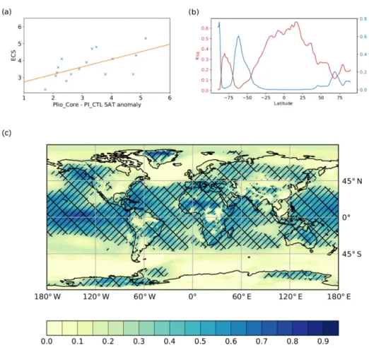
The first analysis of how ECS relates to ESS will con-sider the correlation between ECS and the globally averaged PlioCore–PICtrltemperature anomaly. This is seen in Fig. 7a,
and each cross represents the results from a different model in the PlioMIP2 ensemble. There is a significant relationship between ECS and the PlioCore–PICtrl temperature anomaly
at the 95 % confidence level (p = 0.01, R2=0.35) with the line of best fit being ECS = 2.3 + (0.44 × (PlioCore(SAT) −
PICtrl(SAT))).
Next, we investigate whether there is a correlation across the ensemble between ECS and the PlioCore–PICtrl SAT
anomaly on spatial scales. In the analysis that follows, we will simply assess whether such a correlation exists and, if so, how strong it is by looking at p values and R-squared values calculated from the models in the ensemble. Figure 7b shows the relationship (p value – blue, R squared – red) across the ensemble between modelled ECS and the mod-elled zonal mean PlioCore–PICtrlSAT anomaly. We find a
sig-nificant relationship (p < 0.05) between ECS and the zonal mean Pliocene temperature anomaly throughout most of the tropics. This relationship becomes significant at the 99 % confidence level (p < 0.01) between 38◦N and 27◦S, where a high proportion of the inter-model variability in global ECS can be related to the inter-model variability in the Pliocene
Figure 6.(a) The NH averaged precipitation anomaly for each PlioMIP2 model and for each month with the dashed black line showing the PlioMIP2 multi-model mean. The grey shaded region shows the range of values obtained from PlioMIP1 with the PlioMIP1 multi-model mean shown by the dotted black line. (b) The ratio of the precipitation anomaly over land to the precipitation anomaly over sea for each PlioMIP2 model. Analogous results from individual PlioMIP1 models are shown by the thin grey lines. A ratio of 1.0, where the land precipitation anomaly is the same as the sea precipitation anomaly, is shown in orange.
SAT anomaly at an individual latitude, reaching a maximum of 65 % at ∼ 15◦N.
Next the relationship between global ECS and the local PlioCore–PICtrlSAT anomaly is assessed. In Fig. 7c, colours
show the R-squared correlation across the ensemble be-tween modelled global ECS and the modelled local PlioCore–
PICtrlSAT anomaly. The regions where the relationship
be-tween the two is significant at the 95 % confidence level are hatched. The relationship between ECS and the local PlioCore–PICtrlSAT anomaly is significant over most of the
tropics and over some middle- and high-latitude regions in-cluding Greenland and parts of Antarctica. In many cases, the tropical oceans show a temperature anomaly more strongly related to ECS than the land, although this is not always the case.
4 Data–model comparison
Haywood et al. (2013a, b) proposed that the proxy data and climate model comparison in PlioMIP1 could include dis-crepancies owing to the comparison between time averaged PRISM3D SST and SAT data and climate model represen-tations of a single time slice. In order to improve the in-tegrity of the data–model comparisons in PlioMIP2, Foley and Dowsett (2019) synthesized alkenone SST data that can be confidently attributed to the Marine Isotope Stage (MIS) KM5c time slice that experiment PlioCoreis designed to
rep-resent. Foley and Dowsett (2019) provide two different SST datasets. One dataset includes all SST data for an interval of 10 000 years around the time slice (5000 years to either side of the peak of MIS KM5c), and the other covers 30 000 years (up to 15 000 years to either side of the peak; this latter
dataset will hereafter be referred to as F&D19_30). Age models used in the compilation are those originally released with the datasets, but later modifications of age models or the integration of additional data could result in mean SST values different from those reported in F&D19_30. All SST estimates are calibrated using Müller et al. (1998). Prescott et al. (2014) demonstrated that due to the specific nature of orbital forcing 20 000 years before and after the peak of MIS KM5c, age and site correlation uncertainty within that in-terval would be unlikely to introduce significant errors into SST-based DMC. Given this and in order to maximize the number of ocean sites where SST can be derived, we carry out a point-based SST data–model comparison using the F&D19_30 dataset.
We compare the multi-model mean SST anomaly to a proxy SST anomaly created by differencing the F&D19_30 dataset from observed pre-industrial SSTs derived for years 1870–1899 of the NOAA Extended Reconstructed Sea Sur-face Temperature (ERSST) version 5 dataset (Huang et al., 2017; Fig. 8a and b). Figure 8c shows the proxy data 1SST minus the model mean 1SST. Using the multi-model mean results, 17 of the 37 sites show a difference in data–model 1SST of no greater than ±1◦C (Fig. 8c). These are located mostly in the tropics but also include sites in the North Atlantic, along the coastal regions of California and New Zealand, and in the North Pacific. In terms of discrep-ancies, the clearest and most consistent signal comes from the Benguela upwelling system (off the south-west coast of Africa) where the multi-model mean does not predict the scale of warming seen in three of the four proxy reconstruc-tions. The multi-model mean is insufficiently sensitive in the two Mediterranean Sea sites, along the east coast of North
Figure 7. (a) The globally averaged PlioCore–PICtrl SAT anomaly for each model versus the published equilibrium climate sensitivity (crosses) with the line of best fit shown in orange. (b) Statistical relationships between the latitudinally averaged PlioCore–PICtrlSAT anomaly
and the published climate sensitivity. The proportion of climate sensitivity that can be explained by the SAT anomaly at each latitude (R2) is shown in red, while the probability that there is no correlation between the climate sensitivity and the SAT anomaly (p) is shown in blue. (c) Colours show the percentage variation in modelled ECS that is linearly related to the modelled PlioCore–PICtrlSAT anomaly at each grid
square (R2). Hatching shows a significant relationship (at the 5 % confidence level) between the PlioCore–PICtrlSAT anomaly at that grid
square and ECS.
America (Yorktown Formation) and at one location west of Svalbard close to the sea-ice margin. The multi-model mean predicts a warming that is too great at one location off the Florida and Norwegian coasts. No discernible spatial pattern or structure is seen (outside of the Benguela and Mediter-ranean regions) for sites where the ensemble underestimates or overestimates the magnitude of SST change.
Comparing model-predicted and proxy-based absolute SST estimates for the MIS KM5c time slice (Fig. 8d) yields a similar outcome to the comparison of SST anomalies (Fig. 8c). However, the Benguela region shows greater data– model agreement when considering absolute SSTs than when considering anomalies. Furthermore, a somewhat clearer pic-ture emerges of the model ensemble not producing SSTs that are warm enough in the higher latitudes of the North Atlantic, in the position of the modern North Atlantic gyre and espe-cially in the Nordic Sea, although this appears site dependant as the ensemble overestimates absolute SSTs near Scandi-navia.
The proxy data 1SST minus the mean 1SST for indi-vidual models is shown in Fig. S6. In regions where there was a strong discrepancy between the proxy data 1SST and the multi-model mean 1SST, none of the individual models show good data–model agreement. The EC-Earth3.3 model shows an improved agreement with the data in the Mediter-ranean, the Benguela upwelling system, the site along the east coast of North America and the site to the west of Sval-bard. However, this improved data–model agreement is at the expense of reduced data–model agreement elsewhere; many of the low- and middle-latitude sites which had good data–model agreement for the multi-model mean have re-duced data–model agreement in EC-Earth3.3. Other mod-els which showed great warming in PlioMIP2 (i.e. CESM2 and CCSM4-Utr) also show a larger 1SST than the data for some of the tropical- and middle-latitude sites which were in good agreement with the multi-model mean. Mod-els that were less sensitive to Pliocene boundary conditions (i.e. GISS2.1G and NorESM-L) do not predict the amount of
Figure 8.(a) PRISM4–NOAA ERSSTv5 SST anomaly for the data points described in Sect. 4. (b) Multi-model mean PlioCore–PICtrl
SST anomaly at the points where data are available. (c) The difference between the SST anomaly derived from the data (a) and that of the multi-model mean (b). (d) The PRISM4 SST data minus the PlioCoremulti-model mean.
warming seen in the data for some of the North Atlantic sites, and the multi-model means performs better. Table 3 shows statistics for the data–model comparison for both individual models and the multi-model mean. The root mean square er-ror (RMSE) between the model and the data is 3.72 for the multi-model mean but is lower in some individual models (namely CESM2, IPSLCM6A, EC-Earth3.3, CESM1.2 and CCSM4-UoT). In general, those models that have a lower data–model RMSE are those which have a higher ECS and a higher PlioCore–PICtrlwarming, while less sensitive models
have a higher model data RMSE. The average difference be-tween the data and model across all the data points shows a similar pattern. The proxy data are on average 1.5◦C warmer than the multi-model mean. However, some individual mod-els have a much smaller average data–model discrepancy (e.g. CESM2 = −0.18◦C). The models with a lower data– model discrepancy are those which also have a lower data– model RMSE and have higher than average PlioCore–PICtl
warming.
This initial analysis suggests that the most sensitive mod-els agree better with the proxy data than the less sensitive models. However, further analysis does not fully support this result. If we consider how many of the 37 sites have
“good” data–model agreement, a different picture emerges. Table 3 shows how many sites have model 1SST within 2, 1 and 0.5◦C of the data 1SST. Using these diagnostics, the multi-model mean (MMM) performs better than any of the 16 individual models. Those models which have the low-est RMSE and the blow-est average data–model agreement are not those models which have the largest number of sites where model and data agree. For example, CESM2 and EC-Earth3.3 have a particularly low number of sites with good data–model agreement. The models with the highest num-ber of sites with data–model agreements (e.g. ISPLCM6A, CCSM4-UoT, MIROC4m and CESM1.2) show a PlioCore–
PICtl warming that is closer to the MMM. The fact that
the MMM has more sites with “good” data–model agree-ment than any individual model highlights the benefit of per-forming a large multi-model ensemble as we have done for PlioMIP2. It allows inherent biases within individual mod-els to cancel out and likely provides a more accurate way of estimating climate anomalies than can be done with a single model.
Models show a strong relationship between SST anoma-lies and global mean SAT anomaanoma-lies (Fig. S7a; SATanom = (1.18 × SSTA) + 0.66, Rsq = 0.97) and also a strong