HAL Id: hal-01954676
https://hal.sorbonne-universite.fr/hal-01954676
Submitted on 13 Dec 2018HAL is a multi-disciplinary open access
archive for the deposit and dissemination of sci-entific research documents, whether they are pub-lished or not. The documents may come from teaching and research institutions in France or abroad, or from public or private research centers.
L’archive ouverte pluridisciplinaire HAL, est destinée au dépôt et à la diffusion de documents scientifiques de niveau recherche, publiés ou non, émanant des établissements d’enseignement et de recherche français ou étrangers, des laboratoires publics ou privés.
Nitrous oxide emissions from inland waters: Are IPCC
estimates too high?
Taylor Maavara, Ronny Lauerwald, Goulven Laruelle, Zahra Akbarzadeh,
Nicholas Bouskill, Philippe van Cappellen, Pierre Régnier
To cite this version:
Taylor Maavara, Ronny Lauerwald, Goulven Laruelle, Zahra Akbarzadeh, Nicholas Bouskill, et al.. Nitrous oxide emissions from inland waters: Are IPCC estimates too high?. Global Change Biology, Wiley, In press. �hal-01954676�
Accepted
Article
DR. TAYLOR MAAVARA (Orcid ID : 0000-0001-6677-9262) MS. ZAHRA AKBARZADEH (Orcid ID : 0000-0002-9555-4772)
Article type : Primary Research Articles
Nitrous oxide emissions from inland waters: Are IPCC estimates too high?
Taylor Maavara1,2, Ronny Lauerwald2,3, Goulven G. Laruelle2,4,5, Zahra Akbarzadeh6, Nicholas
J. Bouskill1, Philippe Van Cappellen6, Pierre Regnier2
1
Earth and Environmental Sciences Area, Lawrence Berkeley National Laboratory, Berkeley, California 94720, USA
2
Department Geoscience, Environment & Society, Université Libre de Bruxelles, Brussels, 1050, Belgium
3
Department of Mathematics, College of Engineering, Mathematics and Physical Sciences, University of Exeter, Exeter EX4 4QE, UK
4
UMR 7619 Metis, Sorbonne Universités, UPMC, Univ Paris 06, CNRS, EPHE, IPSL, Paris, France
5
FR636 IPSL, Sorbonne Universités, UPMC, Univ Paris 06, CNRS, Paris, France
6 Ecohydrology Research Group, Water Institute, and Department of Earth and
Environmental Sciences, University of Waterloo, Waterloo, Ontario N2L 3G1, Canada
Accepted
Article
Corresponding author: Taylor Maavara (tmaavara@lbl.gov)
Abstract
Nitrous oxide (N2O) emissions from inland waters remain a major source of uncertainty in
global greenhouse gas budgets. N2O emissions are typically estimated using emission factors
(EFs), defined as the proportion of the terrestrial nitrogen (N) load to a water body that is
emitted as N2O to the atmosphere. The Intergovernmental Panel on Climate Change (IPCC)
has proposed EFs of 0.25% and 0.75%, though studies have suggested that both these values are either too high or too low. In this work, we develop a mechanistic modeling
approach to explicitly predict N2O production and emissions via nitrification and
denitrification in rivers, reservoirs, and estuaries. In particular, we introduce a water residence time dependence, which kinetically limits the extent of denitrification and nitrification in water bodies. We revise existing spatially-explicit estimates of N loads to inland waters to predict both lumped watershed and half-degree grid cell emissions and EFs worldwide, as well as the proportions of these emissions that originate from denitrification
and nitrification. We estimate global inland water N2O emissions of 10.6-19.8 Gmol N yr-1
(148-277 Gg N yr-1), with reservoirs producing most N2O per unit area. Our results indicate
that IPCC EFs are likely overestimated by up to an order of magnitude, and that achieving the magnitude of the IPCC’s EFs is kinetically improbable in most river systems.
Denitrification represents the major pathway of N2O production in river systems, whereas
nitrification dominates production in reservoirs and estuaries.
Introduction
Nitrous oxide (N2O) is an ozone-depleting greenhouse gas (GHG), considered to be the third
most important GHG contributing to radiative forcing and global climate change
(Ravishankara et al., 2009; Syakila & Kroeze, 2011; Neubauer & Megonigal, 2015). Most N2O
is produced by microbial processes such as nitrification and denitrification in terrestrial and aquatic systems, including rivers, estuaries, coastal seas and the open ocean (Freing et al.,
2012). The production of N2O shows large spatial and temporal variability and emission
estimates for aquatic systems are uncertain. In particular, emissions from rivers, estuaries and continental shelves have been the subject of debate for many years (De Klein et al., 2006; Seitzinger & Kroeze, 1998). The 5th IPCC Assessment Report (Ciais et al., 2013)
proposed that, together, rivers, estuaries and coastal zones emit 0.6 Tg N (N2O) yr-1 (based
on IPCC’s 2006 guidelines, Kroeze et al., 2010; Syakila and Kroeze, 2011). This corresponds
to about 3% of all N2O emissions and about one third of IPCC’s previous estimate of 1.7 Tg N
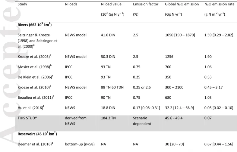
yr-1 in the 4th Assessment Report for the same systems. Several studies have highlighted that
emissions from rivers might be underestimated (Beaulieu et al., 2011) or significantly overestimated (Hu et al., 2016; Macdonald et al., 2016) in the IPCC assessments (Table 1). A recent review of estuarine emissions (Murray et al., 2015) also suggested that these aquatic
Accepted
Article
systems could emit about 3 times more N2O (0.31 Tg N yr-1) than the latest IPCC estimate.
Recently, Deemer et al. (2016) provided the first global estimate of N2O evasion from dam
reservoirs at 0.03 Tg N yr-1.
Global N2O flux estimations from open inland waters (rivers, reservoirs and estuaries) have
followed two distinct approaches. The first approach involves upscaling direct N2O flux
measurements from aquatic systems, by multiplying local fluxes by the estimated global areal extents of water bodies. This methodology has been followed by Deemer et al. (2016) for reservoirs and by Bange (2006), Law et al. (1992), Robinson et al. (1998), de Wilde and de Bie (2000), and Murray et al. (2015) for estuaries. To our knowledge, this approach has
never been applied to estimate river N2O emissions globally. The most recent global N2O
budgets rely on 58 local measurements in reservoirs (Deemer et al., 2016) and 74 local measurements in estuarine environments (Murray et al., 2015) including open waters, mangroves, intertidal sediments, salt marshes and seagrasses. According to Murray et al.
(2015), about 75% of the estuarine N2O evasion originates from open water bodies, i.e. the
portion of estuaries flooded throughout the entire tidal cycle. In addition to the uncertainties associated with using a limited pool of data to generate global estimates, uncertainties arise from the highly skewed spatial distributions of the local datasets, which are focused in industrialized countries, and from the uncertainties associated with the estimated areal extents of different types of water bodies (Dürr et al., 2011; Laruelle et al., 2013; Lehner et al., 2011).
The second approach for estimating large-scale N2O emissions relies on semi-empirical
models, in which N2O emission rates are calculated as the product of an emission factor (EF)
and estimates of N loading to water bodies. However, both N load estimates and EFs are subject to large uncertainties. In particular, EFs (generally defined as the fraction of N load
to the water body that is emitted as N2O-N) vary by more than one order of magnitude, with
reported values ranging from 0.17 to 5.6% (Beaulieu et al., 2011; Hu et al., 2016; Seitzinger & Kroeze, 1998). Several studies argue that the current default IPCC EF used to estimate worldwide emissions (0.25%) may be either overestimated (Clough et al., 2011; Clough et al., 2007; Kroeze et al., 2010) or underestimated (Beaulieu et al., 2011; Yu et al., 2013). Much of the disagreement arises from local values differing substantially from IPCC’s default EF values, due to factors such as intense urbanization (where there may be disproportionately high emissions, e.g. Yu et al., 2013) or diurnal variability (where in-stream concentrations decrease at night, indicating that the majority of studies that sample during the day may overestimate emissions e.g. Clough et al., 2007). Kroeze et al. (2010) further discuss the uncertainty associated with whether the EF is taken with regard to total N (TN) or dissolved inorganic N (DIN) loads to the water body (Table 1), as TN includes
Accepted
Article
refractory N species while DIN excludes other bioavailable species. Inconsistencies in assumptions and methodologies such as these confound our ability to make direct comparisons between literature estimations.
Model-derived estimates of global N2O evasion require inclusion of natural as well as
anthropogenic N loadings, of which the anthropogenic loadings are dominant in most river systems (Seitzinger et al., 2000). For rivers, loadings have been constrained using the IPCC methodology (Mosier et al., 1998), which assumes that the only TN sources are from global synthetic fertilizer use and N excreted by livestock, with 30% lost to leaching and surface runoff. The Global Nutrients in Watersheds (NEWS) model (Dumont et al., 2005; Mayorga et al., 2010) computes DIN and TN loadings according to empirical relationships between loading and an array of controlling factors including biophysical watershed characteristics, population density, socioeconomics, land cover and land use, and climatic conditions.
Discrepancies in N2O evasion between studies can partly be explained by different N load
estimates (Table 1). For estuaries, only the NEWS model approach has been used, with the inputs derived from the NEWS loads delivered to coastal zones (Seitzinger et al., 2005; Seitzinger & Kroeze, 1998).
All model studies scale the global N2O emissions to the N loads, either considering only DIN
(Beaulieu et al., 2011; Hu et al., 2016; Seitzinger & Kroeze, 1998), or including dissolved inorganic, organic and particulate N forms (DIN + DON + PN = TN) together (Mosier et al., 1998; Syakila & Kroeze, 2011). This upscaling can either be done directly by applying an EF to the N load following the IPCC methodology of Mosier et al. (1998), or via an intermediate step (Seitzinger & Kroeze, 1998) where N loads are first used to constrain global
denitrification and nitrification rates and, next, N2O emissions are assumed to be fixed
fractions of these N transformation pathways. Nevertheless, the second approach is somewhat equivalent to the first because all studies have so far assumed that the N lost via denitrification and the N oxidized via nitrification are themselves fixed fractions of TN or DIN loadings (Beaulieu et al., 2011; Seitzinger & Kroeze, 1998).
By far, most of the differences in model-derived estimates result from the choice of
prescribed fractions of N loads which are lost in the form of N2O, either via the direct
approach or via the intermediate step of estimated denitrification-nitrification rates. With the notable exception of the recent study by Hu et al. (2016), all studies have applied EFs and fractions determined from a very limited number of observations, and their values have thus been subject to intense debate in past decades. Interestingly, the proposed EF of Hu et
al. (2016), based on a meta-analysis of 169 N2O flux observations covering a wide range of
Accepted
Article
N that is oxidized via nitrification has been traditionally scaled to denitrification rates, but the scaling factor has varied between 1 and 2 among various studies (Kroeze et al., 2005; Seitzinger & Kroeze, 1998; Seitzinger et al., 2000).
All models applied thus far have relied on simple semi-empirical approaches. As pointed out by Ivens et al. (2011), alternative approaches that better account for spatial variability and model uncertainties should be developed. More specifically, developing a global-scale mechanistic model that represents both N cycling and transport rates in a spatially- and dynamically-explicit way remains a critical priority. Such a mechanistic model should include
representations of nitrification, denitrification and N assimilation rates, as well as N2O
inputs from land and N2O production and transport along the river system (Ivens et al.,
2011). This objective is particularly timely because Beaulieu et al. (2011) have recently
reported denitrification N2O yields (percentage of denitrified N released as N2O) for a
number of streams and rivers (n=72) that can be used to parameterize a mechanistic modeling approach.
In a first step in this direction, we have developed the first integrated model of global N2O
emissions along the entire land-ocean aquatic continuum (LOAC). We focus our study on open waters, including rivers, dammed reservoirs, and estuaries. This analysis does not include lakes or wetlands including freshwater wetlands, seagrasses, salt marshes, intertidal sediments, mangroves, or coastal aquaculture ponds. We calculate DIN, DON, and PN yields in watersheds worldwide, and track the changes to these species’ loads as they are delivered to rivers, reservoirs, and estuaries. We quantify cascading TN losses via burial and
denitrification, and additions via N fixation. In each water body, we quantify the N2O
emissions associated with in-stream, in-estuarine or in-reservoir denitrification and nitrification. We contextualize the results of our model by performing a scenario-based uncertainty analysis, which relies on the range of emissions factors reported in the existing literature. We further compare to existing global estimates for both anthropogenic and
natural N2O emissions. Through our explicit quantification of the interacting changes of N
loads along the LOAC and of the load-specific N2O production mechanisms, our study
represents the most comprehensive estimate of LOAC N2O emissions to date.
Materials and Methods
Overview
A mechanistic mass balance model was developed to represent generalized stream, reservoir, and estuarine N fluxes and transformations (Figure 1). The model development followed an approach similar to that used for phosphorus (P) (Maavara et al., 2015), organic
Accepted
Article
carbon (OC) (Maavara et al., 2017) and N (Akbarzadeh et al., in review) cycling in dam reservoirs. River, reservoir, and estuary kinetic parameters associated with physical and biogeochemical processes were implemented using probability density functions (PDFs) that account for the global distributions of the corresponding parameter values (Table S1). The fluxes in the model represent lumped sediment-water column rates and were resolved at the annual timescale. Water residence time controls the magnitude of the in-system transformation and elimination fluxes through an inverse relationship with nutrient effluxes
from the water body. The N2O model was coupled to OC and P models of (Maavara et al.,
2015, 2017) in order to represent P- and OC-dependencies into processes such a primary productivity and N fixation.
A Monte Carlo analysis of the model was performed, in which parameters were randomly selected from the pre-assigned PDFs. After 6000 iterations, a database of hypothetical
worldwide N dynamics, including N2O production and emissions, was generated for inland
open waters. Each of the 6000 Monte Carlo realizations combined a unique set of parameter values obtained stochastically from the PDFs to quantify rates and fluxes for all N
cycling processes. Next, global relationships relating N processes and N2O emissions to
water residence time and TN loads were extracted from the Monte Carlo output. These relationships were then applied to N loads delivered to all river, reservoir and estuarine systems along a spatially routed network representing the global LOAC. We predicted N loads following the methods used in the NEWS model and described in Mayorga et al. (2010). Rather than applying an average EF to all water bodies, the use of water residence
time as independent variable explicitly adjusts for the extent of N2O production and
emission that is kinetically possible within the timeframe available in a given water body. In the following sections we describe the modeling steps and parameter constraints in detail.
Emission factors: terminology
Emission factors (EFs) have variable definitions throughout the literature. In this study, we utilize a variety of these literature definitions in addition to our own to develop a suite of
scenarios based on a variety of assumptions related to N2O emissions. Henceforth, the
following EF definitions apply:
(1)
(2)
Accepted
Article
(4) (5) and (6)where is the annual flux of N2O emitted across the water-air interface relative to the
nitrification or denitrification flux, is the annual denitrification flux, is the
annual nitrification flux, is the annual production of N2O in the water body via
nitrification or denitrification, is the annual production of N2O via denitrification
minus the N2O subsequently transformed to N2, and is the annual riverine load of total
N delivered to the water body. In the literature, has typically been used as the
conventional definition.
Mechanistic modeling approach
The N pools in the model were nitrate (NO3-) and ammonium (NH4+), dissolved organic N
(DON) and particulate organic N (PON) pools, and the key transformation and transport fluxes associated with these species (Figure 1). Specifically, we took into account the
influxes and effluxes of NH4+, NO3-, DON and PON to and from water bodies, primary
productivity, PON solubilization and burial, mineralization of DON, nitrification,
denitrification, plus N2O production and consumption via the latter two processes, and N2O
exchanges with the atmosphere. Each model realization was solved using the Runge-Kutta 4 integration method, with a 0.01-year time step and, in the case of reservoirs, run for the number of years since dam closure, or for at least 100 years in the case of rivers and estuaries, hence ensuring steady state conditions were reached under the majority of parameter combinations in the Monte Carlo simulations. We constrained one PDF for rivers, reservoirs, and estuaries as a compiled dataset. In this section, we will focus on describing
the model parameters specifically associated with N2O production and emissions. A full
description of the parameterization of the physical and other biogeochemical processes included in the model can be found in Section S1.
Two approaches were used to bracket our estimates of N2O emissions from inland waters.
Accepted
Article
(7)
In the first, more simple, approach (referred to as Default Scenario 1, or DS1), N2O emissions
were calculated by multiplying average and values of 0.9%,
proposed by Beaulieu et al. (2011), by model-calculated nitrification and denitrification
fluxes (see section S1), assuming all was emitted to the atmosphere. A Monte Carlo
simulation was performed, generating 6000 hypothetical “observations” from which globally applicable relationships were extracted that relate denitrification, nitrification, and
N2O emissions to water residence times and TN loads ( , mol yr-1). Nitrification in rivers,
reservoirs and estuaries was fitted to the following equation:
R2 = 0.16 (8)
where is the fixation flux in mol yr-1, calculated using Equations S6 and S7.
Denitrification was similarly fitted to:
R2
= 0.29 (9)
and were multiplied by for each river,
reservoir and estuary worldwide, where we assumed that and
= .
In the second scenario (Default Scenario 2, or DS2), we explicitly included N2O as a pool in
the model (Figure 1), with Equation 7 representing the input to the N2O pool. To account for
consumption of N2O produced via denitrification in water bodies with long residence times
( , we computed the inverse of Equation 9 and multiplied it by an average value of
of 0.9% (Figure S6). The resulting emission factor associated with denitrification
was therefore:
(10)
With this approach, net N2O production accounted for the interplay between increasing
Accepted
Article
For nitrification, was assumed equal to 0.9% with no further scaling because
there is no N2O consumption step associated with nitrification. We then calculated the
emissions, N2Oem, assuming that only the fraction of N2O that is super-saturated with
respect to the equilibrium atmospheric N2O concentration ([N2O]sat) was emitted. In other
words:
[N2O]sat = KH pN2Oatm (11)
and
N2Oem = ([N2O]aq– [N2O]sat) Q (12)
where [N2O]aq is the concentration of N2O in the water body calculated by the model, and
pN2Oatm is the average atmospheric partial pressure of N2O, equal to 315 ppb in year 2000
(EPA 2016), and KH is the temperature dependent Henry’s Law coefficient, equal to 2.4 x 10⁻⁴
mol m-3 Pa-1 at 298.15 K, and temperature corrected to model-predicted temperatures (see
Section S1) using the Van’t Hoff equation. The gradient between actual and equilibrium concentration is multiplied by the amount of water passing through that system per year Q
[km3 yr-1]. Using this emission estimate, it was possible to back-calculate ,
, and for comparison with literature values. Equations 11 and 12 assume
that, on a yearly time scale, aqueous N2O reaches equilibrium with the atmosphere. (Note:
for shorter times scales, more sophisticated kinetics-based approaches may be more appropriate, e.g. Lauerwald et al., 2017).
A second Monte Carlo simulation was run for DS2, and from the output we fitted a single
equation for the total N2O emissions in rivers, reservoirs and estuaries:
(13)
where a = 0.002277 and b = 1.63 (R2 = 0.11, Figure S1a). Though the literature is divided on
whether emissions should be normalized to the TN or DIN load, we chose to normalize our
estimates of N2O emissions and denitrification to TN because this yielded better fits of the
entire set of equations to the Monte Carlo data than using DIN. The fraction of the total N2O
Accepted
Article
(14)
where c = 0.7789, d = -1.366, and e = 2.751 (R2 = 0.66, Figure S1b). Equation 13 was
multiplied by Equation 14 to obtain the N2O evasion from denitrification. Evasion from
nitrification was then calculated as the difference between total evasion and that associated with denitrification.
Application to global river network
To calculate the cascading loads of TN delivered to each water body along the river-reservoir-estuary continuum, we spatially routed reservoirs from the Global Reservoirs and Dams (GRanD) database (Lehner et al, 2011), with river networks from Hydrosheds 15s (Lehner et al., 2008) and Hydro1K (USGS, 2000) at higher latitudes, which was in turn connected to estuaries as represented in the “Worldwide Typology of Nearshore Coastal Systems” of Dürr et al. (2011). A detailed description of the process used to develop this
global water body network is given in the Section S2 and Figure S2.
To calculate biogeochemical transformation rates and emission fluxes for river reaches, reservoirs and estuaries in a consistent way, the water residence times for each of these water bodies was required. For rivers, the average travel distance (Length, km) along an undammed reach discharging into a reservoir or estuary was estimated using the empirical equation of Rosso et al. (1991):
(15)
where is the undammed catchment area upstream of the kth dam or estuary
in km2. The undammed upstream is defined for each dam and estuary as the
total tributary area from which water flows in without passing another dam. The total upstream areas of all the dams and estuaries were spatially delineated based on the Hydrosheds15s (Lehner et al., 2008) and Hydro1k (USGS, 2000) data sets. They were calculated by subtracting the upstream areas of other dams were overlays occurred. For each dam, the contributing area was derived from the Hydrosheds15s and/or Hydro1k routing schemes. In river catchments with multiple dams, the travel distance of water flowing out of a given dam to the next downstream dam or estuary was calculated as the shortest distance between the dams, or between the dam and the receiving estuary. This
Accepted
Article
distance was multiplied by a sinuosity index of 2.26 (Shen et al., 2017) to estimate the actual travel distance. Next, the water residence time along the given river segment was estimated
by dividing the travel distance by an average flowing velocity of 0.6 m s-1 for tributaries and
0.8 m s-1 for the river mainstem (Schulze et al., 2005).
For reservoirs, the residence time was calculated using the representative storage capacity (volume) divided by the annual discharge reported in GRanD (Lehner et al., 2011). Only dams constructed during or before year 2000 were included. For estuaries, water residence times were derived from the nearshore coastal systems database compiled by Dürr et al. (2011), which includes estuarine residence times from the literature for 130 systems that account for 20% of the world’s TN loads from rivers. Following McKee et al. (2004) it was assumed that most of the biogeochemical processing of material exported by the largest rivers of the world takes place in external river plumes located beyond the boundaries of estuarine systems. The estuarine residence time of such large rivers (e.g. Amazon, Ganges, Zaire…) was thus assumed to be negligible (Dürr et al., 2011; Laruelle et al., 2013). The
remaining estuarine systems with no estimate were assigned type-specific median
residence times for four different geomorphological classes of estuaries (Laruelle at al., 2013). These median residence times were derived from the compiled database and were equal to 0.08, 0.27, 0.78 and 10.2 years for deltas, tidally-dominated estuaries, lagoons and fjords, respectively.
The calculation of N2O emissions from a given water body required computation of TNin,
which accounted for terrestrial inputs and N fixation delivered to the water body, minus the upstream losses by burial and denitrification. Because N fixation (Fix) depends on the
relative availability of P (Equations S6-S7), the computation of N2O fluxes required the full
coupling of the N and P cycles along the river-reservoir-estuary continuum.
Similar to the procedure in Maavara et al. (2017), we obtained the average terrestrial DIN,
DON, PN, DIP, DOP and PP yields (Y in mol km-2 yr-1) from the undammed catchment area
upstream of each dam and estuary from NEWS (Mayorga et al., 2010). However, instead of using the average yield per STN-30p basin as in NEWS, we refined the approach to account for the spatial variability in terrestrial N and P sources within each watershed. Based on the input data used in NEWS (Bouwman et al., 2009; Van Drecht et al., 2009), we reproduced the spatially explicit representation of N and P sources at a 0.5-degree resolution. Nutrient loads to the undammed upstream catchment area of a given reservoir or estuary,
Accepted
Article
(16)
where is the yield for that watershed area (mol km-2 yr-1) and is the
undammed catchment area lying directly upstream of the dam (see section S2).
N inputs along the aquatic continuum via N fixation were calculated using Equations S6 and S7. Losses via denitrification were computed with Equation 9, while burial in reservoirs was calculated using the following equation fitted to the results of the Monte Carlo simulations:
R2
= 0.50 (17)
The global equation derived in Maavara et al. (2015) was used to estimate the corresponding burial fluxes of TP. Reduction of the N load by denitrification and addition via N fixation were calculated for mainstem river reaches transporting N downstream from a dam, yielding an “effective” load to the next downstream reservoir or receiving estuary. N burial in river systems, which primarily takes place in adjacent floodplains, occurs via a different mechanism than reservoirs and we therefore did not generate river residence time-dependent retention equations or attempted to estimate this process (Aufdenkampe et al., 2011).
The net nutrient loads delivered to a given dam or estuary can be summarized as:
(18)
where is the flux into the reservoir or estuary k, is the sum of all
effective fluxes discharging from dams upstream of reservoir or estuary k (if any), and
is the flux from the undammed catchment area, with denitrification and N
fixation accounted for. N2O emissions from undammed river reaches and mainstems
Accepted
Article
To analyze the global spatial patterns in N2O emissions, we mapped the combined emissions
from rivers, reservoirs and estuaries obtained for DS1 and DS2 at 0.5° resolution. In
addition, we plotted the N inputs to the river network and the related N2O emission factors
(EF(d)) at the same resolution. A complete description of the method used to perform these calculations can be found in Section S3.
Scenario-based uncertainty analysis
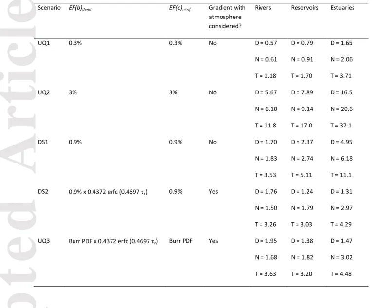
In addition to the N2O emission estimates made in DS1 and DS2, we predicted N2O
emissions according to three supplementary scenarios (UQ1-3, Table 2), which helped to contextualize the existing, often contradictory, observations in the literature. UQ1-3 incorporate various EFs and assumptions reported in the literature and, hence, provide
insights into the uncertainty associated with the predicted N2O emissions.
In UQ1 and UQ2, we followed the same assumptions as DS1, but set
at 3% and 0.3%, respectively, based on Seitzinger and Kroeze (1998). In these
scenarios the transformation of N2O to N2 was not explicitly computed; instead the EFs were
assumed to represent net production, that is, all N2O produced in the water body was
assumed to be emitted to the atmosphere. In UQ3, the emission was calculated as in DS2:
consumption of N2O via denitrification was accounted for (Equation 10) and only
supersaturated N2O was emitted to the atmosphere. Rather than fixing = 0.9%
to scale Equation 10, UQ3 randomly generated values from a Burr distribution
fitted to the Beaulieu et al. (2011) data which range from 0.04 to 5.63%. values
were generated from the same Burr distribution, but independently of
The Monte Carlo analysis was repeated for UQ3, generating an additional set of 6000
hypothetical observations from which relationships relating N2O emissions to water residence
times and TN loads were extracted. Upscaling was performed using the same method as in DS2, whereby fitting of the results of the Monte Carlo analysis to Equations 13 and 14
yielded a = 0.002204, b = 1.955, c = 0.6801, d = -1.131, and e = 2.945 (R2 = 0.04 and 0.57).
Results
Nitrogen input to rivers
According to our re-distributed estimates of allochthonous N inputs to the global river network (after Mayorga et al., 2010; Van Drecht et al. 2009, Bouwman et al., 2009), the
total loading amounts to 13.2 Tmol yr-1 (184.3 Tg N yr-1), of which 4.39 Tmol yr-1 (61.4 Tg N
yr-1) are delivered as DIN, 0.85 Tmol yr-1 (11.9 Tg N yr-1) as DON, and the remaining 2.19
Accepted
Article
supplied from catchment areas that are intercepted by at least one dam. The global spatial pattern of allochthonous N inputs to rivers (Figure 2) is characterized by high yields across Europe, the eastern half of North America and Southern and Eastern Asia, in particular for DIN as the dominant fraction of TN. Low yields are observed for dryer regions of North Africa, Central Asia, and the Western half of North America.
3.1 Nitrification and denitrification fluxes
Worldwide, nitrification fluxes exceed denitrification fluxes in inland waters on average by 5-20%, depending on the system. Global nitrification fluxes in rivers, reservoirs, and
estuaries are 0.20 Tmol yr-1 (2.8 Tg N yr-1), 0.30 Tmol yr-1 (4.3 Tg N yr-1), and 0.69 Tmol yr-1
(9.6 Tg N yr-1), respectively. In comparison, denitrification fluxes are 0.19, 0.26 and 0.55
Tmol yr-1 (2.6, 3.7, and 7.7 Tg N yr-1) for rivers, reservoirs and estuaries, respectively. Upon
averaging each water body or stream segment arithmetically, 0.24% of is nitrified in
rivers, 27% in reservoirs, 22% in estuaries, and 0.22% of is denitrified in rivers, 22% in
reservoirs, and 17% in estuaries. On a per-watershed basis, the Amazon, Ganges, Nile, St. Lawrence, and Mississippi River basins account for 18% and 17% of all the denitrification and nitrification in inland waters worldwide, respectively (Figure S3 and S4), with the Amazon accounting for a third of both values. In what follows, we briefly compare our results with global denitrification fluxes published in the literature. A similar comparison is not possible for nitrification, as there are no previous global scale nitrification flux estimates for inland waters.
Our low denitrification estimate in river systems can partly be explained by the exclusion of denitrification occurring in groundwater and riparian zones (Laursen & Seitzinger, 2002; Marzadri et al., 2017; Saunders & Kalff, 2001) in our modeling approach. Our results predict that the maximum proportion of TN delivered to river reaches that is lost via denitrification is 18%. In existing studies, watershed-scale denitrification losses have been suggested to be as high as 65% using empirical relationships from regional datasets (McCrackin et al., 2014; Seitzinger et al., 2002). However, these studies include the effects of reservoirs in basin-wide budgets, which increases the contribution of denitrification substantially. Indeed, when we account for riverine plus reservoir denitrification, up to 57% of the TN load to river basins is removed via denitrification (with a few exceptions in watersheds with extremely high N fixation), which is in good agreement with the 65% loss cited above. Overall, our results highlight that for most river networks worldwide, N loss via denitrification along undammed river stretches rarely exceeds a few percent, due to their short residence times (median =1.2 days and mean = 4 days; Figure 5).
Accepted
Article
Denitrification rates reported for individual reservoirs vary from 0.01 to 108 g N m-2 yr-1
(David et al., 2006; Grantz et al., 2012; Han et al., 2014; Koszelnik et al., 2007). Local studies have shown that denitrification usually accounts for between 4% and 58% of the elimination
of supplied to reservoirs (David et al., 2006; Garnier et al., 1999; Koszelnik et al., 2007;
Kunz et al., 2011). Globally, only Seitzinger et al. (2006) differentiated between N removal mechanisms in reservoirs, and proposed that denitrification originating from land-derived N
in lakes and reservoirs falls in between 19 to 43 Tg N yr-1, an order of magnitude larger than
our estimates.
Published estimates of the denitrification efficiency (in % N loss) in estuaries vary between
10 and 75% of TNin (An & Joye, 2001; Eyre et al., 2011; Eyre et al., 2016; Nixon et al., 1996;
Seitzinger, 1987; Smyth et al., 2013). However, most systems displaying very high denitrification efficiencies are tropical shallow oligotrophic systems with extensive sea grass coverage (Smyth et al., 2012; Eyre et al., 2016), which are not representative of the global coastline (Dürr et al., 2011). The bulk of the remaining estimates falls in the 10-50% range, which is consistent with our results where estuarine systems characterized by short
residence times of several days like small deltas only denitrify a few percent of TNin, while
systems such as fjords with residence times of several years denitrify up to 38% of TNin. Our
results are also in line with the study of Volta et al. (2016) who used a generic, physically based estuarine modeling approach spanning a wide range of estuarine geometries; these authors report mean N losses via denitrification in the range 15-25%.
3.2 Global N2Oemissions from inland waters
Our results indicate that the IPCC EF(d) values for rivers and estuaries of 0.25% for denitrification only and 0.75% for denitrification plus nitrification (Mosier et al., 1998), or 0.25% for both processes (Ciais et al., 2013), are likely over-estimated. The arithmetically averaged catchment-scale EF(d) values for denitrification plus nitrification are 0.003% for upland tributaries, 0.007-0.008% for river mainstems, 0.17-0.44% for reservoirs and 0.11-0.37% for estuaries, with all values comprised between 0 and 1.2% (note: the ranges given
are for scenarios DS1 and DS2). When calculated by dividing the global N2O emission fluxes
by the global TNin fluxes, the EF(d) values are 0.025-0.027% for rivers, 0.07-0.12% for
reservoirs and 0.062-0.16% for estuaries (Table 1). The two sets of EF(d) differ because the
latter values depend on the TNin fluxes delivered to the water bodies, in addition to the
intrinsic N2O production dynamics of the different types of water bodies. The higher EF(d)
values for reservoirs and estuaries compared to those for rivers dominate the global spatial patterns in simulated EF(d) values (Figure 3). High EF(d) values prevail along the coasts and across North America, Europe, Southern and Eastern Asia, southeast Africa, and eastern Australia, where dams are numerous.
Accepted
Article
We predict worldwide N2O emissions of 10.6-19.8 Gmol N yr-1 (148-277 Gg N yr-1) for inland
waters, 3.03-5.11 Gmol yr-1 (42.4-71.5 Gg N yr-1) for reservoirs, 4.29-11.12 Gmol yr-1
(60.0-156 Gg N yr-1) for estuaries, and 3.26-3.53 Gmol yr-1 (45.6-49.4 Gg N yr-1) for rivers.
Generally, spatial patterns in N2O emission are linked to those of N inputs into river systems
(Figure 2), which explains the high emission rates over the populated areas of North America, Europe, Southeast Asia, and throughout the tropics (Figure 4 and Figure S5). The
global scale spatial patterns of N2O emissions are also clearly influenced by the distribution
of dams and estuaries. However, other factors can also play a role: Arctic rivers such as the Mackenzie and Yenisei Rivers have basins with small TN yields compared to agricultural
watersheds (70th and 33rd percentiles of average yields for all watersheds), but due to the
large residence times, they rank in the top 20 watersheds for emissions.
Discussion
Anthropogenic N2O emissions
Our estimated inland water N2O emissions represent 0.8-1.5% of the 1.28 x 10³ Gmol yr-1 of
N2O-N (17.9 x 10³ Gg N yr-1) emitted worldwide (Ciais et al., 2013). Furthermore, our revised
NEWS estimates predict that 1.14 x 10³ Gmol yr-1 (15.9 Tg N yr-1) of the total dissolved N
(TDN) load to watersheds is anthropogenic in origin, which corresponds to 52% of the TDN load. (Note: we cannot estimate the proportion of the PN load that is anthropogenic in origin using the NEWS model approach, because enhanced erosion of PN from anthropogenic drivers such as deforestation are not accounted for). We can therefore
estimate that 2.6 – 9.9 Gmol yr-1 additional N2O-N is evaded from rivers and estuaries due to
enhanced anthropogenic loading to watersheds (this range assumes that either all or none
of the 14.3 Tg N yr-1 PN load is anthropogenic in origin), which is at least fivefold lower than
Beaulieu et al. (2011) who estimate that 49 Gmol yr-1 (0.68 Tg N yr-1) of anthropogenic N
inputs to river systems are converted to N2O.
We consider all emissions from reservoirs to be anthropogenic. Reservoirs also alter the
riverine fluxes of TN through enhanced denitrification, burial, and fixation, affecting the N2O
emission fluxes downstream of dams. Taking into account the effects of dams, we estimate
that the total human-driven increase in N2O emissions from inland waters, relative to
pre-industrial conditions, falls in the range 5.6–14.5 Gmol N yr-1, or 1.1-3.0% of the 493 Gmol yr
-1
(6.9 Tg N yr-1) anthropogenic N2O emitted worldwide from all sources combined (Ciais et
al., 2013). This flux represents between 23.4 and 60.7 Tg CO2-equiv. yr-1. The upper bound of
our range is larger than the national emissions from any country in Europe. The fact that these are sustained emissions has been shown to be especially problematic from a global warming potential point of view. Neubauer and Megonigal (2015) quantify the global warming potential of sustained emissions, and compared them with pulse fluxes (which is
Accepted
Article
traditionally how global warming potential has been measured). Their results show that
even after 500 years, ecosystems must sequester 181 kg of CO2 to offset 1 kg of N2O
emissions, compared with 132 kg as predicted using the traditional global warming potentials metric.
System-specific emissions efficiencies and mechanisms
By comparing the results of DS1 and DS2, we can evaluate the effect of explicitly accounting
for consumption of N2O during the last step of denitrification in each water body type
(rivers, reservoirs and estuaries). The EF(a) values in Beaulieu et al. (2011) are field
measurements and thus may already have been affected to some degree by N2O
consumption. A comparison of the results of DS1 and DS2 therefore provides some measure
of the uncertainty associated with using the Beaulieu et al. (2011) data to parameterize N2O
emissions in the model calculations. Essentially, in DS1 we assume that the field-based EF
values account for both N2O production and consumption during denitrification, while in
DS2 they do not include the reduction of N2O to N2. Despite the relatively wide ranges
predicted in both default scenarios, the relative trends in predicted emissions are quite
similar. The estimates for both DS1 and DS2 indicate that estuaries emit more N2O
worldwide than reservoirs or river systems, accounting for 41-56% of the total emissions fluxes along the LOAC. This reflects their much larger global areal extent (and
correspondingly, their volume and residence times) of 1067 x 103 km2, compared with the
smaller 45 x 103 km2 surface area of reservoirs and 662 x 103 km2 of rivers (Table 1).
Per unit area, N2O emissions from estuaries and rivers are significantly lower than for
reservoirs: average surface-area-normalized emission rates are 4.0–10.4 x 10⁻³ mol N m-2 yr-1
for estuaries, 4.9-5.3 x 10⁻³ mol N m-2 yr-1 for rivers, and 67.3-114 x 10-3 mol N m-2 yr-1 for
reservoirs. The differences in areal emissions largely reflect the residence time distributions of the water bodies (Figure 5). The median residence time for reservoirs is close to 10 months, corresponding to an EF(d) of 0.3% in DS1 and 0.2% in DS2. Estuaries, by comparison, have a median residence time of about 3 months, which corresponds to an average EF(d) of 0.1% in both scenarios (Figure 5). Water bodies with residence time below
2-3 days, which account for 70% of river systems in our analysis, produce negligible N2O in
both scenarios.
River systems exhibit the lowest emissions of the three systems, directly as a result of their
much lower water residence times. When consumption of N2O via denitrification is explicitly
accounted for in DS2, a larger proportion of N2O emissions originates from denitrification in
Accepted
Article
via denitrification exceeds N2O produced via nitrification (Figure 5). In rivers, 46% of the
global N2O emissions originate from nitrification and 54% from denitrification (Table 2). In
DS2, the average EF(a)denit for rivers is 1.2%, compared with the EF(a)nitrif of 0.76%. By
comparison, in the same scenario at least 59% of emissions in both reservoirs and estuaries
are from nitrification. Hence, in DS2 the N2O emission flux by denitrification for all rivers
worldwide (1.76 Gmol yr-1) exceeds those for reservoirs (1.24 Gmol yr-1) and estuaries (1.31
Gmol yr-1).
The larger role of denitrification as the source of N2O in river systems is not seen for DS1,
where consumption is assumed to have already been accounted for in the EF(a) values
reported by Beaulieu et al. (2011). EF(a)nitrif and EF(a)denit are both fixed at 0.9% in this
scenario, so any differences between emission pathways are due entirely to the relative magnitudes of the denitrification and nitrification fluxes. Nitrification accounts for a slight
majority (52%) of riverine N2O emissions because of the larger nitrification fluxes predicted
at residence times above ~5-6 months (Figure S6). At residence times below 5-6 months, the magnitudes of nitrification and denitrification fluxes are roughly equal (Figure S6), which is
why in rivers, which have low residence times, both N2O production pathways contribute
about the same to the global riverine emissions, compared to rivers and estuaries, where nitrification is the dominant pathway (Table 2). A discussion of the mechanisms driving
spatially explicit N2O emissions, and worldwide hotspots, can be found in Section S4.
Evaluating literature observations
In this section, we first compare our model results with published global-scale N2O emission
estimates for reservoirs and estuaries obtained by scaling up local measurements. We then move on to rivers where previous estimates have all relied on semi-empirical modeling approaches. Additional discussion related to uncertainties in existing literature and field-based studies needed to improve global estimates can be found in Section S5.
Reservoirs and estuaries
Using a bottom-up approach (n = 58), Deemer et al. (2016) obtained a global N2O
emission flux from reservoirs of 2.14 Gmol yr-1 (30 Gg N yr-1). Despite the entirely
different approach, this estimate agrees well with our prediction of 3.03 – 5.11 Gmol yr-1.
Estimates of N2O emissions from estuaries vary greatly from 7 to 407 Gmol yr-1 (100 to
5700 Gg N yr-1, Table 1). It is worth noting that all estimates higher than 43 Gmol N yr-1
(600 Gg N yr-1) were calculated by applying the average emission of a very small number
of estuaries (between 1 and 12) to all estuaries worldwide, possibly implying that the estuaries studied may have disproportionately large emissions relative to the global average. Only the most recent bottom-up estuarine emissions estimate of Murray et al. (2015) and the older estimate of Robinson et al. (1998) overlap with our range of values
Accepted
Article
(Table 1). In contrast, calculations relying on semi-empirical modeling approaches predict
emissions on the order of 7 Gmol N yr-1 (100 Gg N yr-1) that agree with our range of 4.29–
11.1 Gmol N yr-1 (60.0156 Gg N yr-1) (Kroeze et al., 2010; Kroeze et al., 2005; Seitzinger
and Kroeze, 1998; Seitzinger et al., 2000).
Rivers
Published estimates of riverine N2O emissions show the greatest variability of all the
water body types considered (Table 1), with the highest values two orders of magnitude
larger than the lowest ones (32.2 – 2100 Gg N yr-1). All existing river emission estimates
rely on semi-empirical modeling approaches, and thus the differences are entirely dependent on the predicted loads to rivers, the EF values used and, perhaps most importantly, the assumptions made. For all estimates except one, one of the following sets of assumptions applies:
(1) EF(d) = 3% or 0.3%; all of the N load to the river system is nitrified once and half the N
load is denitrified once, i.e. EF(a)nitrif = 2 EF(a)denit = EF(d) (as in Kroeze et al., 2005;
Seitzinger & Kroeze, 1998; Seitzinger et al., 2000);
(2) EF(a)denit = 0.25% and EF(a)nitrif = 0.50%, with EF(a)denit + EF(a)nitrif = 0.75% = EF(d) (as
in Beaulieu et al., 2011; Mosier et al., 1998), or (ii) EF(d) = EF(a)denit = EF(a)nitrif =
0.25% (as in Ciais et al., 2013; De Klein et al., 2006; Kroeze et al., 2010). These values also constitute the IPCC guidelines.
Both of these sets of assumptions, however, fail to consider the kinetic limitations imposed by the short water residence times characteristic of most rivers. In our model scenarios, we apply the same EF(a) values as in the above assumptions but introduce a
water residence time dependence on EF(d). The corresponding river N2O emissions fall
between 1.18 and 11.8 Gmol N yr-1 (16.5-165 Gg N yr-1) (Table 2). These values imply that
rivers likely emit significantly less N2O than proposed in the majority of previous studies,
largely because of the limited amount of time available for nitrification and denitrification to occur in most undammed river reaches.
Seitzinger and Kroeze (1998) predict that 75.1 Gmol N yr-1 of N2O are emitted from rivers,
based on a global DIN load to rivers of 3.0 Tmol yr-1, assuming that TN:DIN = 2:1 and that
watersheds yielding more than 10 kg N ha-1 yr-1 have an EF(d) of 3% while the remainder
have an EF(d) of 0.3%. In comparison, scenarios UQ1 and UQ2, which bracket the EF(d)
range of 3-0.3%, yield riverine emissions of 1.18 – 11.8 Gmol yr-1, with a TN load of 7.42
Accepted
Article
and UQ2, Seitzinger and Kroeze’s riverine N2O emissions far exceed our estimates. We
suggest that the assumed denitrification efficiency in Seitzinger and Kroeze (1998), namely that half the N load to rivers is denitrified, is a severe over-estimation and not attainable for the short residence times in these systems. According to our results, on
average only 0.22% of TNin is denitrified in undammed river segments while, globally,
denitrification in rivers eliminates 1.4% of the total TNin load to watersheds. The large
discrepancy is in part explained by the implicit inclusion of higher residence time water bodies such as reservoirs in the older estimates. However, even when we include reservoirs in our calculations only 19% of the global TN loads to river networks is
denitrified. Beaulieu et al. (2011) assume that all N2O produced in rivers is emitted, i.e.
EF(a) = EF(b) = EF(c) = EF(d) = 0.9%. In DS1 we assume EF(a) = EF(b) = EF(c) = 0.9% but
calculate residence time dependent EF(d) values, which yields a mean EF(d) value of
0.004% and a river N2O emission flux of 3.53 Gmol N yr-1, much smaller than Beaulieu’s
48.6 Gmol N yr-1 estimate.
To our knowledge, the only study that explicitly departs from either of the two sets of assumptions listed above is that of Hu et al. (2016), who included 6200 watersheds in
their analysis. Our predicted riverine emissions in DS1 and DS2 of 3.26 - 3.53 Gmol yr-1
(45.6-49.4 Gg N yr-1), align well with Hu et al.’s prediction of 0.89–4.78 Gmol yr-1 (12.4–
66.9 Gg N yr-1) N2O emissions. While our calculations were performed at a higher spatial
resolution than Hu et al.’s, the general global spatial trends are comparable. In both
studies, the largest hotspot for riverine N2O emissions is Southeast Asia. Furthermore, Hu
et al. (2016) predict that 86% of the riverine N2O outgassing takes place in equatorial and
subtropical regions, which is exactly the proportion of global riverine N2O emissions
between 40°N and 40°S according to our simulations. Other regions characterized by high emission rates include western Europe, the Amazonian basin, central Africa and eastern North America. Hu et al. also suggest that commonly used EF estimates are generally too high. They further estimate that EFs relative to DIN loads are somewhere in the range 0.08-0.31%, based on a statistical analysis in which 82 regression models were tested
against a dataset of 169 measured riverine N2O emissions. Thus, despite using two
entirely independent approaches, both our work and that of Hu et al. support the conclusion that previous EFs are overestimated.
Outlook
Our calculated global N2O emissions from rivers, reservoirs and estuaries fall in the range
10.6-19.8 Gmol N yr-1 (148-277 Gg N yr-1), more than half, and up to an order of magnitude,
lower than most studies based on IPCC’s guidelines. Despite the much reduced N2O flux
estimates, we find that anthropogenic perturbations to river systems have doubled to
Accepted
Article
of 0.25% and 0.75% are too high to be applied across all rivers, estuaries and reservoirs. Instead, we estimate the following ranges of emissions factors: 0.004-0.005% for rivers, 0.17-0.44% for reservoirs, and 0.11-0.37% for estuaries. These values, obtained by arithmetically averaging all individual emission factors for a given water body type, directly reflect the water residence time distributions of rivers, reservoirs and estuaries. The majority of emissions in estuaries and reservoirs originate from nitrification, while denitrification tends to dominate in rivers because of the shorter residence times. We find
that reservoirs are the most efficient N2O emitters on a per-area basis, with average areal
emissions rates an order of magnitude larger than for rivers and estuaries. We therefore
expect worldwide N2O emissions from inland waters to rise substantially in the coming
decades as a result of the ongoing global boom in dam construction (Zarfl et al., 2015), which will nearly double the number of large hydroelectric dams on Earth. A systematic analysis of predicted changes to water residence times caused by these new dams needs to
be conducted to aid in forecasting changes in worldwide N2O emissions.
Acknowledgments
This research received funding from the European Union’s Horizon 2020 research and innovation programs under the Marie Sklodowska-Curie grant agreement no. 643052 (C-CASCADES project) and under a grant agreement no. 776810 (VERIFY project). TM was funded by a Natural Sciences and Engineering Research Council of Canada (NSERC) postdoctoral fellowship (no. PDF-516575-2018), RL received funding from the European Union’s Horizon 2020 research and innovation program under grant agreement no. 703813 for the Marie Sklodowska-Curie European Individual Fellowship ‘C-Leak’, and GL was supported by Labex L-IPSL, which is funded by ANR (grant #ANR-10-LABX-0018). TM and NJB are supported as part of the Watershed Function Scientific Focus Area funded by the U.S. Department of Energy, Office of Science, Office of Biological and Environmental Research under Award Number DE-AC02-05CH11231.
Accepted
Article
References
Akbarzadeh, Z., Maavara, T., Slowinski, S., & Van Cappellen, P. (in review). Effects of damming on river nitrogen fluxes: a global analysis.
An, S., & Joye, S. B. (2001). Enhancement of coupled nitrification‐denitrification by benthic
photosynthesis in shallow estuarine sediments. Limnology and Oceanography, 46(1), 62-74. Aufdenkampe, A. K., Mayorga, E., Raymond, P. A., Melack, J. M., Doney, S. C., Alin, S. R., . . . Yoo, K.
(2011). Riverine coupling of biogeochemical cycles between land, oceans, and atmosphere.
Frontiers in Ecology and the Environment, 9(1), 53-60.
Bange, H. W. (2006). Nitrous oxide and methane in European coastal waters. Estuarine, Coastal and
Shelf Science, 70(3), 361-374.
Barros, N., Cole, J. J., Tranvik, L. J., Prairie, Y. T., Bastviken, D., Huszar, V. L., . . . Roland, F. (2011). Carbon emission from hydroelectric reservoirs linked to reservoir age and latitude. Nature
geoscience, 4(9), 593.
Beaulieu, J. J., Tank, J. L., Hamilton, S. K., Wollheim, W. M., Hall, R. O., Mulholland, P. J., . . . Dahm, C. N. (2011). Nitrous oxide emission from denitrification in stream and river networks.
Proceedings of the National Academy of Sciences, 108(1), 214-219.
Bouwman, A., Beusen, A. H., & Billen, G. (2009). Human alteration of the global nitrogen and phosphorus soil balances for the period 1970–2050. Global biogeochemical cycles, 23(4). Ciais, P., Sabine, C., Bala, G., Bopp, L., Brovkin, V., Canadell, J., . . . Heimann, M. (2013). Carbon and
Other Biogeochemical Cycles. Retrieved from Cambridge, United Kingdom and New York, NY,
USA:
Clough, T., Buckthought, L., Casciotti, K., Kelliher, F., & Jones, P. (2011). Nitrous oxide dynamics in a braided river system, New Zealand. Journal of environmental quality, 40(5), 1532-1541. Clough, T. J., Buckthought, L. E., Kelliher, F. M., & Sherlock, R. R. (2007). Diurnal fluctuations of
dissolved nitrous oxide (N2O) concentrations and estimates of N2O emissions from a spring‐fed river: implications for IPCC methodology. Global change biology, 13(5), 1016-1027.
David, M. B., Wall, L. G., Royer, T. V., & Tank, J. L. (2006). Denitrification and the nitrogen budget of a reservoir in an agricultural landscape. Ecological Applications, 16(6), 2177-2190.
De Klein, C., Novoa, R. S., Ogle, S., Smith, K. A., Rochette, P., Wirth, T. C., . . . Walsh, M. (2006). N2O emissions from managed soils, and CO2 emissions from lime and urea application. IPCC
Guidelines for National Greenhouse Gas Inventories, Prepared by the National Greenhouse Gas Inventories Programme, 4, 1-54.
de Wilde, H. P., & de Bie, M. J. (2000). Nitrous oxide in the Schelde estuary: production by nitrification and emission to the atmosphere. Marine Chemistry, 69(3-4), 203-216.
Accepted
Article
Deemer, B. R., Harrison, J. A., Li, S., Beaulieu, J. J., DelSontro, T., Barros, N., . . . Vonk, J. A. (2016). Greenhouse gas emissions from reservoir water surfaces: a new global synthesis. BioScience,
66(11), 949-964.
Diem, T., Koch, S., Schwarzenbach, S., Wehrli, B., & Schubert, C. (2012). Greenhouse gas emissions (CO2, CH4, and N2O) from several perialpine and alpine hydropower reservoirs by diffusion and loss in turbines. Aquatic sciences, 74(3), 619-635.
Dumont, E., Harrison, J., Kroeze, C., Bakker, E., & Seitzinger, S. (2005). Global distribution and sources of dissolved inorganic nitrogen export to the coastal zone: Results from a spatially explicit, global model. Global biogeochemical cycles, 19(4).
Dürr, H. H., Laruelle, G. G., van Kempen, C. M., Slomp, C. P., Meybeck, M., & Middelkoop, H. (2011). Worldwide typology of nearshore coastal systems: defining the estuarine filter of river inputs to the oceans. Estuaries and Coasts, 34(3), 441-458.
Eyre, B. D., Ferguson, A. J., Webb, A., Maher, D., & Oakes, J. M. (2011). Denitrification, N-fixation and nitrogen and phosphorus fluxes in different benthic habitats and their contribution to the nitrogen and phosphorus budgets of a shallow oligotrophic sub-tropical coastal system (southern Moreton Bay, Australia). Biogeochemistry, 102(1-3), 111-133.
Eyre, B. D., Maher, D. T., & Sanders, C. (2016). The contribution of denitrification and burial to the nitrogen budgets of three geomorphically distinct Australian estuaries: Importance of seagrass habitats. Limnology and Oceanography, 61(3), 1144-1156.
Fearnside, P. M., & Pueyo, S. (2012). Greenhouse-gas emissions from tropical dams. Nature Climate
Change, 2(6), 382-384.
Freing, A., Wallace, D. W., & Bange, H. W. (2012). Global oceanic production of nitrous oxide.
Philosophical Transactions of the Royal Society of London B: Biological Sciences, 367(1593),
1245-1255.
Garnier, J., Leporcq, B., Sanchez, N., & Philippon, X. (1999). Biogeochemical mass-balances (C, N, P, Si) in three large reservoirs of the Seine Basin (France). Biogeochemistry, 47(2), 119-146. Grantz, E. M., Kogo, A., & Scott, J. T. (2012). Partitioning whole‐lake denitrification using in situ
dinitrogen gas accumulation and intact sediment core experiments. Limnology and
Oceanography, 57(4), 925-935.
Guérin, F., Abril, G., Tremblay, A., & Delmas, R. (2008). Nitrous oxide emissions from tropical hydroelectric reservoirs. Geophysical Research Letters, 35(6).
Han, H., Lu, X., Burger, D. F., Joshi, U. M., & Zhang, L. (2014). Nitrogen dynamics at the sediment– water interface in a tropical reservoir. Ecological Engineering, 73, 146-153.
Hargreaves, J. A. (1998). Nitrogen biogeochemistry of aquaculture ponds. Aquaculture, 166(3-4), 181-212.
Accepted
Article
Hart, R., & Rayner, N. (1994). Temperature-related distributions of Metadiaptomus and Tropodiaptomus (Copepoda: Calanoida), particularly in southern Africa Studies on the
Ecology of Tropical Zooplankton (pp. 77-86): Springer.
Hu, M., Chen, D., & Dahlgren, R. A. (2016). Modeling nitrous oxide emission from rivers: a global assessment. Global change biology, 22(11), 3566-3582.
Islam, M. S. (2005). Nitrogen and phosphorus budget in coastal and marine cage aquaculture and impacts of effluent loading on ecosystem: review and analysis towards model development.
Marine pollution bulletin, 50(1), 48-61.
Ivens, W. P., Tysmans, D. J., Kroeze, C., Löhr, A. J., & van Wijnen, J. (2011). Modeling global N 2 O emissions from aquatic systems. Current opinion in environmental sustainability, 3(5), 350-358.
Janssens-Maenhout, G., Crippa, M., Guizzardi, D., Muntean, M., Schaaf, E., Olivier, J., . . . Schure, K. (2017). Fossil CO2 and GHG emissions of all world countries (1831-9424). Retrieved from Luxembourg:
Koszelnik, P., Tomaszek, J. A., & Gruca-Rokosz, R. (2007). The significance of denitrification in relation to external loading and nitrogen retention in a mountain reservoir. Marine and
Freshwater Research, 58(9), 818-826.
Kroeze, C., Dumont, E., & Seitzinger, S. (2010). Future trends in emissions of N2O from rivers and estuaries. Journal of Integrative Environmental Sciences, 7(S1), 71-78.
Kroeze, C., Dumont, E., & Seitzinger, S. P. (2005). New estimates of global emissions of N2O from rivers and estuaries. Environmental Sciences, 2(2-3), 159-165.
Kunz, M. J., Anselmetti, F. S., Wüest, A., Wehrli, B., Vollenweider, A., Thüring, S., & Senn, D. B. (2011). Sediment accumulation and carbon, nitrogen, and phosphorus deposition in the large tropical reservoir Lake Kariba (Zambia/Zimbabwe). Journal of Geophysical Research:
Biogeosciences, 116(G3).
Laruelle, G. G., Durr, H. H., Lauerwald, R., Hartmann, J., Slomp, C. P., Goossens, N., & Regnier, P. A. G. (2013). Global multi-scale segmentation of continental and coastal waters from the
watersheds to the continental margins. Hydrology and Earth System Sciences, 17(5), 2029-2051. doi:10.5194/hess-17-2029-2013
Lauerwald, R., Regnier, P., Camino-Serrano, M., Guenet, B., Guimberteau, M., Ducharne, A., . . . Ciais, P. (2017). ORCHILEAK (revision 3875): a new model branch to simulate carbon transfers along the terrestrial–aquatic continuum of the Amazon basin. Geoscientific Model
Development, 10(10), 3821.
Laursen, A. E., & Seitzinger, S. P. (2002). Measurement of denitrification in rivers: an integrated, whole reach approach. Hydrobiologia, 485(1-3), 67-81.
Law, C., Rees, A., & Owens, N. (1992). Nitrous oxide: estuarine sources and atmospheric flux.
Accepted
Article
Lehner, B., Liermann, C. R., Revenga, C., Vorosmarty, C., Fekete, B., Crouzet, P., . . . Wisser, D. (2011). High-resolution mapping of the world's reservoirs and dams for sustainable river-flow management. Frontiers in Ecology and the Environment, 9(9), 494-502. doi:10.1890/100125 Lehner, B., Verdin, K., & Jarvis, A. (2008). New global hydrography derived from spaceborne
elevation data. Eos, Transactions American Geophysical Union, 89(10), 93-94.
Maavara, T., Parsons, C. T., Ridenour, C., Stojanovic, S., Dürr, H. H., Powley, H. R., & Van Cappellen, P. (2015). Global phosphorus retention by river damming. Proc Natl Acad Sci U.S.A., 112(51), 15603-15608.
Maavara, T., Lauerwald, R., Regnier, P., & Van Cappellen, P. (2017). Global perturbation of organic carbon cycling by river damming. Nature Communications, 8: 15347.
Macdonald, B., Nadelko, A., Chang, Y., Glover, M., & Warneke, S. (2016). Contribution of the cotton irrigation network to farm nitrous oxide emissions. Soil Research, 54(5), 651-658.
Marzadri, A., Dee, M. M., Tonina, D., Bellin, A., & Tank, J. L. (2017). Role of surface and subsurface processes in scaling N2O emissions along riverine networks. Proceedings of the National
Academy of Sciences, 114(17), 4330-4335.
Mayorga, E., Seitzinger, S. P., Harrison, J. A., Dumont, E., Beusen, A. H. W., Bouwman, A. F., . . . Van Drecht, G. (2010). Global Nutrient Export from WaterSheds 2 (NEWS 2): Model development and implementation. Environmental Modelling & Software, 25(7), 837-853.
doi:10.1016/j.envsoft.2010.01.007
McCrackin, M. L., Harrison, J. A., & Compton, J. E. (2014). Factors influencing export of dissolved inorganic nitrogen by major rivers: A new, seasonal, spatially explicit, global model. Global
biogeochemical cycles, 28(3), 269-285.
McKee, B., Aller, R., Allison, M., Bianchi, T., & Kineke, G. (2004). Transport and transformation of dissolved and particulate materials on continental margins influenced by major rivers: benthic boundary layer and seabed processes. Continental Shelf Research, 24(7-8), 899-926. Mosier, A., Kroeze, C., Nevison, C., Oenema, O., Seitzinger, S., & Van Cleemput, O. (1998). Closing the
global N2O budget: nitrous oxide emissions through the agricultural nitrogen cycle. Nutrient
cycling in Agroecosystems, 52(2-3), 225-248.
Murray, R. H., Erler, D. V., & Eyre, B. D. (2015). Nitrous oxide fluxes in estuarine environments: response to global change. Global change biology, 21(9), 3219-3245.
Neubauer, S. C., & Megonigal, J. P. (2015). Moving beyond global warming potentials to quantify the climatic role of ecosystems. Ecosystems, 18(6), 1000-1013.
Nixon, S., Ammerman, J., Atkinson, L., Berounsky, V., Billen, G., Boicourt, W., . . . Elmgren, R. (1996). The fate of nitrogen and phosphorus at the land-sea margin of the North Atlantic Ocean.