Design of computer experiments: space filling and beyond

HAL Id: hal-00685876

https://hal.archives-ouvertes.fr/hal-00685876

Submitted on 6 Apr 2012

HAL is a multi-disciplinary open access

archive for the deposit and dissemination of

sci-entific research documents, whether they are

pub-lished or not. The documents may come from

teaching and research institutions in France or

abroad, or from public or private research centers.

L’archive ouverte pluridisciplinaire HAL, est

destinée au dépôt et à la diffusion de documents

scientifiques de niveau recherche, publiés ou non,

émanant des établissements d’enseignement et de

recherche français ou étrangers, des laboratoires

publics ou privés.

beyond

Luc Pronzato, Werner Müller

To cite this version:

Luc Pronzato, Werner Müller. Design of computer experiments: space filling and beyond. Statistics

and Computing, Springer Verlag (Germany), 2012, 22 (3), pp.681-701. �10.1007/s11222-011-9242-3�.

�hal-00685876�

Statistics and Computing manuscript No. (will be inserted by the editor)

Design of computer experiments: space filling and beyond

Luc Pronzato · Werner G. M¨uller

January 28, 2011

Abstract When setting up a computer experiment, it has become a standard practice to select the inputs spread out uniformly across the available space. These so-called space-filling designs are now ubiquitous in cor-responding publications and conferences. The statisti-cal folklore is that such designs have superior properties when it comes to prediction and estimation of emula-tor functions. In this paper we want to review the cir-cumstances under which this superiority holds, provide some new arguments and clarify the motives to go be-yond space-filling. An overview over the state of the art of space-filling is introducing and complementing these results.

Keywords Kriging · entropy · design of experiments · space-filling · sphere packing · maximin design · minimax design

This work was partially supported by a PHC Amadeus/OEAD Amad´ee grant FR11/2010.

L. Pronzato

Laboratoire I3S, Universit´e de Nice-Sophia Antipolis/CNRS

bˆatiment Euclide, les Algorithmes

2000 route des lucioles, BP 121 06903, Sophia Antipolis cedex, France Tel.: +33-4-92942703

Fax: +33-4-92942896 E-mail: pronzato@i3s.unice.fr

Werner G. M¨uller

Department of Applied Statistics, Johannes-Kepler-University

Linz Freist¨adter Straße 315, A-4040 Linz, Austria

Tel.: +43-732-24685880 Fax: +43-732-24689846 E-mail: werner.mueller@jku.at

1 Introduction

Computer simulation experiments (see, e.g., Santner et al (2003); Fang et al (2005); Kleijnen (2009)) have now become a popular substitute for real experiments when the latter are infeasible or too costly. In these experiments, a deterministic computer code, the sim-ulator, replaces the real (stochastic) data generating process. This practice has generated a wealth of statis-tical questions, such as how well the simulator is able to mimic reality or which estimators are most suitable to adequately represent a system.

However, the foremost issue presents itself even be-fore the experiment is started, namely how to deter-mine the inputs for which the simulator is run? It has become standard practice to select these inputs such as to cover the available space as uniformly as possible, thus generating so called space-filling experimental de-signs. Naturally, in dimensions greater than one there are alternative ways to produce such designs. We will therefore in the next sections (2,3) briefly review the most common approaches to space-filling design, tak-ing a purely model-free stance. We will then (Sect. 4) investigate how these designs can be motivated from a statistical modelers point of view and relate them to each other in a meaningful way. Eventually we will show that taking statistical modeling seriously will lead us to designs that go beyond space-filling (Sect. 5 and 6). Special attention is devoted to Gaussian process models and kriging. The only design objective considered corre-sponds to reproducing the behavior of a computer code over a given domain for its input variables. Some basic principles about algorithmic constructions are exposed in Sect. 7 and Sect. 8 briefly concludes.

The present paper can be understood as a survey focussing on the special role of space-filling designs and

at the same time providing new illuminative aspects. It intends to bring the respective sections of Koehler and Owen (1996) up to date and to provide a more statistical point of view than Chen et al (2006). 2 State of the art on space-filling design 2.1 Geometric criteria

There is little ambiguity on what constitutes a space-filling design in one dimension. If we define an exact design ξ = (x1, . . . , xn) as a collection of n points and

consider a section of the real line as the design space, say X = [0, 1] after suitable renormalization, then, de-pending upon whether we are willing to exploit the edges or not, we have either xi = (i − 1)/(n − 1) or

xi= (2i − 1)/(2n) respectively.

The distinction between those two basic cases comes from the fact that one may consider distances only amongst points in the design ξ or to all points in the set X. We can carry over this notion to the less straight-forward higher dimensional case d > 1, with now ξ = (x1, . . . , xn). Initially we need to define a proper norm

k.k on X = [0, 1]d_{, Euclidean distances and}

normaliza-tion of the design space will not impede generality for our purposes. We shall denote

dij = kxi− xjk

the distance between the two design points xi and xj

of ξ. We shall not consider the case where there exist constraints that make only a subset of [0, 1]d

admissi-ble for design, see for instance Stinstra et al (2003) for possible remedies; the construction of Latin hypercube designs (see Sect. 2.2) with constraints is considered in (Petelet et al, 2010).

Let us first seek for a design that wants to achieve a high spread solely amongst its support points within the design region. One must then attempt to make the smallest distance between neighboring points in ξ as large as possible. That is ensured by the maximin-distance criterion (to be maximized)

φM m(ξ) = min i6=j dij.

We call a design that maximizes φM m(·) a

maximin-distance design, see Johnson et al (1990). An example is given in Fig. 1–left. This design can be motivated by setting up the tables in a restaurant such that one wants to minimize the chances to eavesdrop on another party’s dinner talk.

In other terms, one wishes to maximize the radius of n non-intersecting balls with centers in X. When X is a d-dimensional cube, this is equivalent to packing rigid

Fig. 1 Maximin (left, see http://www.packomania.com/ and minimax (right, see Johnson et al (1990)) distance designs for n=7 points in [0, 1]2_{. The circles have radius φ}

M m(ξ)/2 on the

left panel and radius φmM(ξ) on the right one.

spheres X, see Melissen (1997, p. 78). The literature on sphere packing is rather abundant. In dimension d = 2, the best known results up to n = 10 000 for finding the maximum common radius of n circles which can be packed in a square are presented on http://www. packomania.com/ (the example on Fig. 1–left is taken from there, with φM m(ξ) ' 0.5359, indicating that the

7-point design in (Johnson et al, 1990) is not a maximin-distance design); one may refer to (Gensane, 2004) for best-known results up to n = 32 for d = 3.

Among the set of maximin-distance designs (when there exist several), a maximin-optimal design ξ∗

M m is

such that the number of pairs of points (xi, xj) at the

distance dij = φM m(ξM m∗ ) is minimum (several such

designs can exist, and measures can be taken to remove draws, see Morris and Mitchell (1995), but this is not important for our purpose).

Consider now designs ξ that attempt to make the maximum distance from all the points in X to their closest point in ξ as small as possible. This is achieved by minimizing the minimax-distance criterion

φmM(ξ) = max

x∈Xminxi

kx − xik .

We call a design that minimizes φmM(·) a

minimax-distance design, see Johnson et al (1990) and Fig. 1– right for an example. (Note the slight confusion in ter-minology as it is actually minimaximin.) These designs can be motivated by a table allocation problem in a restaurant, such that a waiter is as close as possible to a table wherever he is in the restaurant.

In other terms, one wishes to cover X with n balls of minimum radius. Among the set of minimax-distance designs (in case several exist), a minimax-optimal de-sign ξ∗

mM maximizes the minimum number of xi’s such

that minikx − xik = φmM(ξmM∗ ) over all points x

2.2 Latin hypercubes

Note that pure space-filling designs such as ξ∗ mM and

ξ∗

M m may have very poor projectional properties; that

is, they may be not space-filling on any of their mean-ingful subspaces, see Fig. 1. The opposite is desirable for computer experiments, particularly when some inputs are of no influence in the experiment, and this property was called noncollapsingness by some authors (cf. Stin-stra et al (2003)). This requirement about projections is one of the reasons that researches have started to restrict the search for designs to the class of so-called Latin-hypercube (Lh) designs, see McKay et al (1979), which have the property that any of their one-dimensio-nal projections yields the maximin distance sequence

xi = (i − 1)/(n − 1). An additional advantage is that

since the generation of Lh-designs as a finite class is computationally rather simple, it has become custom-ary to apply a secondcustom-ary, e.g. space-filling, criterion to them, sometimes by a mere brute-force enumera-tion as in (van Dam, 2007). An example of minimax and simultaneously maximin Lh design is presented in Fig. 2 (note that there is a slight inconsistency about minimax-Lh designs in that they are maximin rather than minimax on their one-dimensional projections).

Other distances than Euclidean could be considered; when working within the class of Lh designs the situa-tion is easier with the L1 or L∞ norms than with the

L2 norm, at least for d = 2, see van Dam et al (2007);

van Dam (2007). The class of Lh designs is finite but large. It contains (n!)d−1 _{different designs (not (n!)}d

since the order of the points is arbitrary and the first co-ordinates can be fixed to {xi}1= (i − 1)/(n − 1)), and

still (n!)d−1_{/(d−1)! if we consider designs as equivalent}

when they differ by a permutation of coordinates. An exhaustive search is thus quickly prohibitive even for moderate values of n and d. Most algorithmic methods are of the exchange type, see Sect. 7. In order to re-main in the class of Lh designs, one exchange-step corre-sponds to swapping the j-th coordinates of two points, which gives (d − 1)n(n − 1)/2 possibilities at each step (the first coordinates being fixed). Another approach that takes projectional properties into account but is not restricted to the class of Lh designs will be pre-sented in Sect. 3.3. Note that originally McKay et al (1979) have introduced Lh designs as random sampling procedures rather than candidates for providing fixed designs, those random designs being not guaranteed to have good space-filling properties. Tang (1993) has in-troduced orthogonal-array-based Latin hypercubes to improve projections on higher dimensional subspaces, the space-filling properties of which were improved by Leary et al (2003). The usefulness of Lh designs in

Fig. 2 Minimax-Lh and simultaneously maximin-Lh

dis-tance design for n=7 points in [0, 1]2_{, see http://www.}

spacefillingdesigns.nl/. The circles have radius φM m(ξ)/2 on

the left panel and radius φmM(ξ) on the right one.

model-based (as discussed in Sect. 4) examples was demonstrated in (Pebesma and Heuvelink, 1999). The algorithmic construction of Lh designs that optimize a discrepancy criterion (see Sect. 2.3) or an entropy based criterion (see Sect. 3.3) is considered respectively in (Iooss et al, 2010) and (Jourdan and Franco, 2010); the algebraic construction of Lh designs that minimize the integrated kriging variance for the particular cor-relation structure C(u, v; ν) = exp(−νku − vk1) (see

Sect. 4.1) is considered in (Pistone and Vicario, 2010). 2.3 Other approaches to space-filling

There appear a number of alternative approaches to space-filling in the literature, most of which can be sim-ilarly distinguished by the stochastic nature of the in-puts, i.e. whether ξ is to be considered random or fixed. For the latter, natural simple designs are regular grids. Such designs are well suited for determining ap-propriate model responses and for checking whether as-sumptions about the errors are reasonably well satis-fied. There seems little by which to choose between e.g. a square grid or a triangular grid; it is worth noting, however, that the former may be slightly more conve-nient from a practical standpoint (easier input determi-nation) but that the latter seems marginally more effi-cient for purposes of model based prediction (cf. Yfantis et al (1987)).

Bellhouse and Herzberg (1984) have compared op-timum designs and uniform grids (in a one-dimensional model based setup) and they come to the conclusion that (depending upon the model) predictions for cer-tain output regions can actually be improved by reg-ular grids. A comparison in a multi-dimensional setup including correlations can be found in (Herzberg and Huda, 1981).

For higher dimensional problems, Bates et al (1996) recommend the use of (non-rectangular) lattices rather than grids (they also reveal connections to model-based

approaches). In the two-dimensional setup (on the unit square [−1, 1]2_{) the Fibonacci lattice (see Koehler and}

Owen (1996)) proved to be useful. The advantage of lat-tices is that their projection on lower dimensions covers the design region more or less uniformly. Adaptations to irregular design regions may not be straightforward, but good enough approximations will suffice. This is not the case for many other systematic designs that are frequently proposed in the literature, such as central composite designs, the construction of which relies on the symmetry of the design region.

It is evident that randomization can be helpful for making designs more robust. On a finite grid X with

N candidate points we can think of randomization as

drawing a single design ξ according to a pre-specified probability distribution π(·). The uniform distribution then corresponds to simple random sampling and more refined schemes (e.g., stratified random sampling, see Fedorov and Hackl (1997)), can be devised by altering

π(·). A comparison between deterministic selection and

random sampling is hard to make, since for a finite sam-ple it is evident that for any single purpose it is possible to find a deterministic design that outperforms random sampling. Performance benchmarking for various space-filling designs can be found in (Johnson et al, 2008) and (Bursztyn and Steinberg, 2006).

All of the methods presented above seem to ensure a reasonable degree of overall coverage of the study area. However, there have been claims (see e.g. Fang and Wang (1993)), that the efficiency (with respect to coverage) of these methods may be poor when the num-ber of design points is small. To allow for comparisons between designs in the above respect Fang (1980) (see also Fang et al (2000)) introduced some formal criteria, amongst them the so-called discrepancy

D(ξ) = max

x∈X|Fn(x) − U (x)| . (1)

Here U (·) is the c.d.f. of the uniform distribution on X and Fn(·) denotes the empirical c.d.f. for ξ. The

discrepancy by this definition is just the Kolmogorov-Smirnov test statistic for the goodness-of-fit test for a uniform distribution. Based upon this definition, Fang and Wang (1993) suggest to find ‘optimum’ designs of given size n that minimize D(ξ), which they term the U-criterion. For d = 1 and X = [0, 1], the minimax-optimal design ξ∗

mM with xi= (2i − 1)/(2n) is optimal

for (1), with D(ξ∗

mM) = 1/(2n). Note, however, that

D(ξ) ≥ 0.06 log(n)/n for any sequence of n points, see

Niederreiter (1992, p. 24). It turns out that for cer-tain choices of n lattice designs are U-optimum. Those lattice designs are also D-optimum for some specific Fourier regressions and this and other connections are explored by Riccomagno et al (1997). An example in

(Santner et al, 2003, Chap. 5) shows that the measure of uniformity expressed by D(ξ) is not always in agree-ment with common intuition.

Niederreiter (1992) has used similar concepts for the generation of so called low discrepancy sequences. Originately devised for the use in Quasi Monte Carlo sampling, due to the Koksma-Hlawka inequality in nu-merical integration, their elaborate versions, like Faure, Halton and Sobol sequences, are increasingly used in computer experiments (see, e.g., Fang and Li (2006)). Santner et al (2003, Chap. 5) and Fang et al (2005, Chap. 3) provide a good overview of the various types of the above discussed designs and their relations. Other norms than k · k∞ can be used in the definition of

dis-crepancy, yielding Dp(ξ) =

¡R

X|Fn(x) − U (x)|pdx

¢1/p

, and other types of discrepancy (centered, wrap-around) may also be considered. Low discrepancy sequences pre-sent the advantage that they can be constructed se-quentially (which is not the case for Lh designs), al-though one should take care of the irregularity of dis-tributions, see Niederreiter (1992, Chap. 3) and Fang et al (2000) (a conjecture in number theory states that

D(ξn) ≥ cd[log(n)]d−1/n for any sequence ξn with cd a

constant depending on d). It seems, however, that de-signs obtained by optimizing a geometric space-filling criterion are preferable for moderate values of n and that, for n large and d > 1, the space-filling properties of designs corresponding to low-discrepancy sequences may not be satisfactory (the points presenting some-times alignments along subspaces). Note that (Bischoff and Miller, 2006) and related work reveal (in the one-dimensional setup) relationships between uniform de-signs and dede-signs that reserve a portion of the observa-tions for detecting lack-of-fit for various classical design criteria.

2.4 Some properties of maximin and minimax optimal designs

Notice that for any design ξ, X ⊂ ∪n

i=1B(xi, φmM(ξ)),

with B(x, R) the ball with center x and radius R. There-fore, φmM(ξ) > [vol(X)/(nVd)]1/d = (nVd)−1/d, with

Vd= πd/2/Γ (d/2 + 1) the volume of the d-dimensional

unit ball. One may also notice that for any ξ, n ≥ 2,

φmM(ξ) > φM m(ξ)/2 since X cannot be covered with

non-overlapping balls. A sort of reverse inequality holds for optimal designs. Indeed, take a maximin-optimal design ξ∗

M m and suppose that φmM(ξ∗M m) >

φM m(ξM m∗ ). It means that there exists a x∗ ∈ X such

that minikx∗− xik > φM m(ξ∗M m). By substituting x∗

for a xiin ξM m∗ such that dij = φM m(ξM m∗ ) for some j,

de-crease the number of pairs of design points at distance

φM m(ξM m∗ ), which contradicts the optimality of ξM m∗ .

Therefore, φmM(ξM m∗ ) ≤ φM m(ξM m∗ ).

Both φM m(ξM m∗ ) and φmM(ξ∗mM) are non-increasing

functions of n when X = [0, 1]d _{(there may be equality}

for different values of n, for instance, φM m(ξ∗M m) =

√

2 for n = 3, 4 and d = 3, see Gensane (2004)). This is no longer true, however, when working in the class of Lh designs (see e.g. van Dam (2007) who shows that

φmM(ξmM∗ ) is larger for n = 11 than for n = 12 when

d = 2 for Lh designs).

The value of φM m(·) is easily computed for any

de-sign ξ, even when n and the dimension d get large, since we only need to calculate distances between n(n − 1)/2 points in Rd_.

The evaluation of the criterion φmM(·) is more

dif-ficult, which explains why a discretization of X is of-ten used in the literature. It amounts at approximating

φmM(ξ) by ˜φmM,N(ξ) = maxx∈XNminikx − xik, with XN a finite grid of N points in X. Even so, the

calcula-tion of ˜φmM,N(ξ) quickly becomes cumbersome when N

increases (and N should increase fast with d to have a fine enough grid). It happens, however, that basic tools from computational geometry permit to reduce the cal-culation of maxx∈Xminikx − xik to the evaluation of

minikzj− xik for a finite collection of points zj ∈ X,

provided that X is the d-dimensional cube [0, 1]d_{. This}

does not seem to be much used and we detail the idea hereafter.

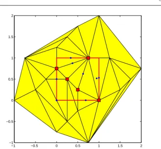
Consider the Delaunay tessellation of the points of

ξ, see, e.g., Okabe et al (1992); Boissonnat and Yvinec

(1998). Each simplex has its d + 1 vertices at design points in the tessellation and has the property that its circumscribed sphere does not contain any design point in its interior. We shall call those circumscribed spheres Delaunay spheres. When a solution x∗ of the problem

maxx∈Xminikx−xik is in the interior of [0, 1]d, it must

be the center of some Delaunay sphere.

There a slight difficulty when x∗is on the boundary

of X, since the tessellation directly constructed from the xidoes not suffice. However, x∗is still the center of

a Delaunay sphere if we construct the tessellation not only from the points in ξ but also from their symmetric with respect to all (d − 1)-dimensional faces of X, see Appendix A.

The Delaunay tessellation is thus constructed on a set of (2d + 1)n points. (One may notice that X is not necessarily included in the convex hull of these points for d ≥ 3, but this is not an issue.) Once the tessellation is calculated, we collect the radii of Delaunay spheres having their center in X (boundary included); the value of φmM(ξ) is given by the maximum of these radii (see

−1 −0.5 0 0.5 1 1.5 2 −1 −0.5 0 0.5 1 1.5 2

Fig. 3 Delaunay triangulation for a 5-point Lh design (squares), the 8 candidate points for being solution of maxx∈Xminikx−xik are indicated by dots.

Appendix A for the computation of the radius of the circumscribed sphere to a simplex).

Efficient algorithms exist for the computation of De-launay tessellations, see Okabe et al (1992); Boissonnat and Yvinec (1998); Cignoni et al (1998) and the refer-ences therein, which make the computation of φmM(ξ)

affordable for reasonable values of d and n (the number of simplices in the Delaunay tessellation of M points in dimension d is bounded by O(Mdd/2e_{)). Clearly, not}

all 2dn symmetric points are useful in the construction, leaving open the possibility to reduce the complexity of calculations by using less than (2d + 1)n points.

Fig. 3 presents the construction obtained for a 5-point Latin-hypercube design in dimension 2: 33 trian-gles are constructed, 11 centers of circumscribed circles belong to X, with some redundancy so that only 8 dis-tinct points are candidate for being solution of the max-imization problem maxx∈Xminikx − xik. The solution

is at the origin and gives φmM(ξ) = minikxik ' 0.5590.

3 Model-free design

We continue for the moment to consider the situation when we are not able, or do no want, to make an as-sumption about a suitable model for the emulator. We investigate the properties of some geometric and other model-free design criteria more closely and make con-nections between them.

3.1 Lq-regularization of the maximin-distance criterion

Following the approach in Appendix B, one can de-fine regularized forms of the maximin-distance

crite-rion, valid when q > 0 for any ξ such that φM m(ξ) > 0: φ_[q](ξ) =  X i<j d−q_ij   −1/q , φ[q](ξ) =  X i<j µijd−qij   −1/q ,

with µij> 0 for all i and

P

i<jµij= 1, see (33, 34). The

criterion φ_[q](·) satisfies φ_[q](ξ) ≤ φM m(ξ) ≤ φ[q](ξ) ≤

µ−1/q_φ

[q](ξ) , q > 0 , with µ = mini<jµij, and the

convergence to φM m(ξ) is monotonic in q from both

sides as q → ∞. Taking µ as the uniform measure, i.e., µij = µ =

¡_n

2

¢−1

for all i < j, gives φ[q](·) =

µ−1/q_φ [q](·) and φ_[q](ξ) ≤ φM m(ξ) ≤ µ n 2 ¶1/q φ_[q](ξ) . (2) It also yields the best lower bound on the maximin ef-ficiency of an optimal design ξ∗_[q] for φ_[q](·),

φM m(ξ∗_[q]) φM m(ξM m∗ ) ≥ µ n 2 ¶−1/q , (3) where ξ∗

M m denotes any maximin-distance design, see

Appendix B. One may define φ_{[N N,0]}(ξ) as

φ[0](ξ) = exp    µ n 2 ¶−1  X i<j log(dij)      (4)

and φ_[2](·) corresponds to a criterion initially proposed by Audze and Eglais (1977). Morris and Mitchell (1995) use φ_[q](·) with different values of q and make the ob-servation that for moderate values of q (say, q - 5) the criterion is easier to optimize than φM m(·) in the

class of Lh designs. They also note that, depending on the problem, one needs to take q in the range 20-50 to make the two criteria φ_[q](·) and φM m(·) agree about

the designs considered best. Their observation is con-sistent with the efficiency bounds given above. Accord-ing to the inequality (3), to ensure that the maximin efficiency of an optimal design for φ_[q](·) is larger than 1 − ² one should take approximately q > 2 log(n)/² (in-dependently of the dimension d). Note that the use of

φ_[q](ξ) = [P_i6=jd−q_ij ]−1/q_{would worsen the maximin}

ef-ficiency bounds by a factor 2−1/q_{< 1 (but leaves φ}

[q](·)

unchanged when the uniform measure µij = [n(n −

1)]−1 _{is used).}

We may alternatively write φM m(ξ) as

φM m(ξ) = min i d

∗

i, (5)

where d∗

i = minj6=idij denotes the nearest-neighbor

(NN) distance from xito another design point in ξ.

Fol-lowing the same technique as above, a Lq-regularization

applied to the min function in (5) then gives

φ_{[N N,q]}(ξ) ≤ φM m(ξ) ≤ n1/qφ_{[N N,q]}(ξ) = φ[N N,q](ξ) (6) with φ_{[N N,q]}(ξ) = " _n X i=1 (d∗ i)−q #−1/q . (7)

The reason for not constructing φ_{[N N,q]}(ξ) from the de-composition φM m(ξ) = miniminj>idij is that the

re-sulting criterion [Pn_i=1(minj>idij)−q]−1/q depends on

the ordering of the design points. One may also define

φ_{[N N,0]}(ξ) as φ[N N,0](ξ) = exp ( 1 n " _n X i=1 log(d∗ i) #) , (8)

see Appendix B. One can readily check that using the generalization (36) with φ(t) = log(t) and q = −1 also gives φ_{[N N,−1,log]}(ξ) = φ_{[N N,0]}(ξ). Not surprisingly,

φ_{[N N,q]}(·) gives a better approximation of φM m(·) than

φ_[q](ξ): an optimal design ξ∗_{[N N,q]}for φ_{[N N,q]}(·) satisfies

φM m(ξ∗_{[N N,q]})

φM m(ξ∗M m)

≥ n−1/q

which is larger than 1 − ² when q > log(n)/², compare with (3). Exploiting the property that, for a given i,

 X j6=i d−q_ij   −1/q ≤ d∗ i ≤ (n − 1)1/q  X j6=i d−q_ij   −1/q ,

see (35), we obtain that

2−1/qφ_[q](ξ) ≤ φ_{[N N,q]}(ξ) ≤ φM m(ξ) φM m(ξ) ≤ n1/qφ_{[N N,q]}(ξ) ≤ µ n 2 ¶1/q φ_[q](ξ) .

Note that the upper bounds on φM m(·) are sharp (think

of a design with n = d + 1 points, all at equal distance from each other, i.e., such that dij = d∗i is constant).

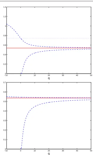
Fig. 4 presents the bounds (2) (dashed lines, top) and (6) (dashed lines, bottom) on the value φM m(ξ)

(solid line) for the 7-point maximin-distance design of Fig. 1–left. Notice the accuracy of the upper bound

n1/q_φ

[N N,q](ξ) (note the different scales between the

top and bottom panels); the situation is similar for other maximin-distance designs since d∗

i = φM m(ξM m∗ )

−100 0 10 20 30 40 50 0.2 0.4 0.6 0.8 1 1.2 1.4 q −100 0 10 20 30 40 50 0.1 0.2 0.3 0.4 0.5 0.6 0.7 q

Fig. 4 Upper and lower bounds (dashed lines) on the value

φM m(ξ) for the 7-point maximin-distance design of Fig. 1–left:

(2) on the top, (6) on the bottom; the value of φM m(ξ) is

indi-cated by a solid line, φ[0](ξ) (4) and φ[N N,0](ξ) (8) are in dotted

lines, respectively on the top and bottom panels.

Oler (1961) indicates that for d = 2 φM m(ξM m∗ ) ≤

[1 + q

1 + 2 (n − 1) /√3]/(n − 1). The equivalence with sphere-packing gives φM m(ξ∗M m) < [(n Vd)1/d/2 − 1]−1

with Vd the volume of the d-dimensional unit ball; this

bound becomes quite loose for large d and can be im-proved by using results on packing densities of dens-est known packings (which may be irregular for some

d > 3), yielding φM m(ξ∗M m) ≤ (31/4 p n/2 − 1)−1 _for d = 2 and φM m(ξM m∗ ) ≤ [(n/ √ 2)1/3_{− 1)}−1 _{for d = 3.}

Bounds for maximin Lh designs in dimension d can be found in (van Dam et al, 2009).

3.2 Lq-regularization of the minimax-distance criterion

The same type of relaxation can be applied to the cri-terion φmM(ξ). First, φ(x) = minxikx − xik is approx-imated by φq(x) = (

P

ikx − xik−q)−1/q with q > 0.

Second, when X is discretized into a finite grid XN =

{x(1)_{, . . . , x}(N )_{}, max} x∈XNφq(x) = [minx∈XNφ −1 q (x)]−1 can be approximated by [PN_j=1φp q(x(j))]1/pwith p > 0.

This gives following substitute for φmM(ξ),

φ[p,q](ξ) =    N X j=1 " _n X i=1 kx(j)− xik−q #−p/q_  1/p

with p, q > 0, see Royle and Nychka (1998). Note that the xi are usually elements of XN. When X is not

dis-cretized, the sum over x(j) _{∈ X}

N should be replaced

by an integral over X, which makes the evaluation of

φ[p,q](ξ) rather cumbersome.

3.3 From maximin-distance to entropy maximization Suppose that the n points xi in ξ form n i.i.d. samples

of a probability measure with density ϕ with respect to the Lebesgue measure on X. A natural statistical approach to measure of the quality of ξ in terms of its space-filling properties is to compare it in some way with samples from the uniform measure on X. Using discrepancy is a possibility, see Sect. 2.3. Another one relies on the property that the uniform distribution has maximum entropy among all distributions with finite support. This is the approach followed in this section.

The R´enyi (1961) entropy of a random vector of Rd

having the p.d.f. ϕ (that we shall call the R´enyi entropy of ϕ) is defined by H∗ α(ϕ) = 1 1 − αlog Z Rd ϕα_{(x) dx , α 6= 1 . (9)}

The Havrda-Charv´at (1967) entropy (also called Tsallis (1988) entropy) of ϕ is defined by Hα(ϕ) = 1 α − 1 µ 1 − Z Rd ϕα(x) dx ¶ , α 6= 1 . (10) When α tends to 1, both Hαand Hα∗tend to the

(Boltz-mann-Gibbs-) Shannon entropy

H1(ϕ) = −

Z

Rd

ϕ(x) log[ϕ(x)] dx . (11)

Note that H∗

α= log[1 − (α − 1)Hα]/(1 − α) so that, for

any α, d(H∗

α)/d(Hα) > 0 and the maximizations of Hα∗

and Hα are equivalent; we can thus speak indifferently

of α-entropy maximizing distributions.

The entropy Hα is a concave function of the

den-sity ϕ for α > 0 (and convex for α < 0). Hence, α-entropy maximizing distributions, under some specific constraints, are uniquely defined for α > 0. In particu-lar, the α-entropy maximizing distribution is uniform under the constraint that the distribution is finitely supported. The idea, suggested by Franco (2008), is thus to construct an estimator of the entropy of the

design points xi in ξ, considering them as if

indepen-dently drawn with some probability distribution, and use this entropy estimator as a design criterion to be maximized. Note that this use of entropy (for a dis-tribution in the space of input factors) is not directly connected Maximum-Entropy Sampling of Sect. 4.3 (for a distribution in the space of responses).

Many methods exist for the estimation of the en-tropy of a distribution from i.i.d. samples, and one may refer for instance to the survey papers (Hall and Mor-ton, 1993; Beirlant et al, 1997) for an overview. We shall consider three, because they have either already been used in the context of experimental design or are directly connected with other space-filling criteria. In a fourth paragraph, entropy decomposition is used to avoid the collapsing of design points when considering lower dimensional subspaces.

Plug-in method based on kernel density estimation The

approach is in two steps. First, one construct an esti-mator of the p.d.f. ϕ by a kernel method as

ˆ ϕn(x) = 1 n hd n n X i=1 K µ x − xi hn ¶ , (12)

where K(·) denotes the kernel and hnthe window width.

The choices of K(·) and hn are important issues when

the objective is to obtain an accurate estimation of ϕ and there exists a vast literature on that topic. How-ever, this should not be too critical here since we only need to get an entropy estimator that yields a reason-able space-filling criterion. A common practice in den-sity estimation is to take hn decreasing with n, e.g. as

n−1/(d+4)_{, see Scott (1992, p. 152), and to use a p.d.f.}

for K(·), e.g. that of the standard normal distribution in Rd_{. A kernel with bounded support could be more}

indicated since X is bounded, but the choice of the win-dow width might then gain importance. When a kernel-based prediction method is to be used, it seems natural to relate K(·) and hn to the kernel used for prediction

(to the correlation function in the case of kriging); this will be considered in Sect. 4.3.

In a second step, the entropy H∗

αor Hαis estimated

by replacing the unknown ϕ by the estimate ˆϕn in the

definition. In order to avoid the evaluation of multi-dimensional integrals, a Monte-Carlo estimator can be used, namely ˆHn

1 = −

P_n

i=1log[ ˆϕn(xi)] for Shannon

entropy, and ˆ Hαn= 1 α − 1 " 1 − n X i=1 ˆ ϕα−1n (xi) # (13) for Hα with α 6= 1. A surprising result about normal

densities is that when K(·) is the p.d.f. of the normal

N (0, I), then Z Rd ˆ ϕ2 n(x) dx = 1 2d_πd/2_n2_hd n X i,j exp · −kxi− xjk 2 4h2 n ¸ ; that is, a Monte-Carlo evaluation gives the exact value of the integral in (9, 10) for ϕ = ˆϕn when α = 2.

This is exploited in (Bettinger et al, 2008, 2009) for the sequential construction of an experiment with the objective of inverting an unknown system.

Nearest-neighbor (NN) distances The following

estima-tor of Hα(ϕ) is considered in (Leonenko et al, 2008)

ˆ Hn,k,α= 1 −[(n−1) CkVd]1−α n Pn i=1(d∗k,i)d(1−α) α − 1 (14)

where Vd = πd/2/Γ (d/2 + 1) is the volume of the unit

ball B(0, 1) in Rd_{, C}

k = [Γ (k)/Γ (k + 1 − α)]1/(1−α)

and d∗

k,i is the k-th nearest-neighbor distance from xi

to some other xj in the sample (that is, from the n − 1

distances dij, j 6= i, we form the order statistics d∗1,i=

d∗

i ≤ d∗2,i≤ · · · ≤ d∗n−1,i). The L2-consistency of this

es-timator is proved in (Leonenko et al, 2008) for any α ∈ (1, (k+1)/2) when k ≥ 2 (respectively α ∈ (1, 1+1/[2d]) when k = 1) if f is bounded. For α < 1, one may refer to (Penrose and Yukich, 2011) for the a.s. and L2

conver-gence of ˆHn,k,αto Hα(ϕ); see also the results of Yukich

(1998) on the subadditivity of Euclidean functionals. For α = 1 (Shannon entropy), the following estima-tor is considered in (Kozachenko and Leonenko, 1987; Leonenko et al, 2008) ˆ HN,k,1= d n N X i=1 log d∗

k,i+ log(n − 1) + log(Vd) − Ψ (k) ,

where Ψ (z) = Γ0_{(z)/Γ (z) is the digamma function.}

Maximizing ˆHn,1,α for α > 1 thus corresponds to

maximizing φ_{[N N,q]}(ξ) with q = d(α − 1), see (7). For 1 − 1/d ≤ α ≤ 1, the criterion ˆHn,1,α, is still eligible

for space-filling, its maximization is equivalent to that

of φ_{[N N,q]}(ξ) with q ∈ [−1, 0]; for instance, the

maxi-mization of ˆHN,1,1is equivalent to the maximization of

φ[N N,0](ξ), see (8).

Several comments should be made, however, that will temper the feeling that Lq-regularization of

maxi-min-distance design and maximization of NN-estimates of entropy are equivalent.

First, these estimators rely on the assumption that the xi are i.i.d. with some p.d.f. ϕ. However,

optimiz-ing the locations of points with respect to some de-sign criterion makes the corresponding sample com-pletely atypical. The associated value of the estima-tor is therefore atypical too. Consider for instance the

maximin-distance design ξ∗

M mon [0, 1], defined by xi=

(i − 1)/(n − 1), i = 1, . . . , n. Direct calculation gives ˆ

Hn,1,α(ξM m∗ ) = [1 − 21−α/Γ (2 − α)]/(α − 1), which

is greater than 1 for 0 < α < 2, with a maximum

γ + log(2) ' 1.2704 when α tends to 1. On the other

hand, the maximum value of H(ϕ) for ϕ a p.d.f. on [0, 1] is obtained for the uniform distribution ϕ∗_{(x) = 1}

for all x, with H(ϕ∗_{) = 0.}

Second, even if the design points in ξ are generated randomly, using k-th NN distances with k > 1 does not make much sense in terms of measuring the space-filling performance. Indeed, when using ˆHn,k,α with k > 1, a

design obtained by fusing sets of k points will show a higher entropy than a design with all points separated. This is illustrated by the simple example of a maximin-distance design on the real line. For the design ξ∗

M m

with n points we have ˆ Hn,2,α(ξ∗M m) = 1 − 21−α Γ (3−α) h 1 +2(21−α_n−1)i α − 1 .

Suppose that n = 2m and consider the design ˜ξ∗ M m

obtained by duplicating the maximin-distance design with m points; that is, xi= (i−1)/(m−1), i = 1, . . . , m,

and xi = (i − m − 1)/(m − 1), i = m + 1, . . . , 2m. We get ˆ Hn,2,α(˜ξ∗M m) = 1 − 21−α Γ (3−α) h 2 + 1 m−1 i1−α α − 1 and ˆHn,2,α(˜ξM m∗ ) > ˆHn,2,α(ξM m∗ ) for α ∈ (0, 3). We

should thus restrict our attention to ˆHn,k,αwith k = 1.

The range of values of α for which the strong consis-tency of the estimator is ensured is then restricted to

α < 1 + 1/[2d]. Strictly speaking, it means that the

maximization of φ_{[N N,q]}(ξ) can be considered as the maximization of a NN entropy estimator for q < 1/2 only.

Minimum-spanning-tree Redmond and Yukich (1996);

Yukich (1998) use the subadditivity of some Euclidean functionals on graphs to construct strongly consistent estimators of H∗

α(ϕ) (9) for 0 < q < 1, up to some

bias term independent of ϕ and related to the graph properties. Their approach covers the case of the graph of k-th NN (where the bias constant depends on the value of k through Ck, see (14)), but also the graphs

corresponding to the solution of a travelling salesman problem, or the minimum spanning tree (MST). In each case, the entropy estimate is based on PM_i=1 dd(1−α)_i , where the di denote the lengthes of the M edges of the

graph, with M = n − 1 for the MST and M = n for the traveling-salesman tour and NN graphs.

The MST constructed from the xihas already been

advocated as a useful tool to assess the quality of de-signs in terms of their space-filling properties: in (Franco et al, 2009), the empirical mean and variance of the lengthes of edges di of the MST are used to

character-ize classes of designs (such as random, low discrepancy sequences, maximin-distance and minimax-distance de-signs); designs with large empirical means are consid-ered preferable. With the same precautions as above for NN entropy estimation, the maximization of the func-tion (Pn−1_i=1 d−q_i )−1/q _{in the MST constructed from the}

xiis related to the maximization of an entropy

estima-tor of the distribution of the xi; in particular, the

max-imization of the empirical mean of the edge lengthes (q = −1) forms a reasonable objective.

Entropy decomposition to avoid collapsing on projec-tions Let u and v be two independent random vectors

respectively in Rd1 and Rd2. Define x = (u>, v>)> and

let ϕ(u, v) denote the joint density for x. Let ϕ1(u)

and ϕ2(v) be the marginal densities for u and v

respec-tively, so that ϕ(u, v) = ϕ1(u)ϕ2(v). It is well known

that the Shannon and R´enyi entropies (11) and (9) sat-isfy the additive property H∗

α(ϕ) = Hα∗(ϕ1) + Hα∗(ϕ2),

α ∈ R (extensivity property of Shannon and R´enyi

entropies) while for the Tsallis entropy (10) one has

Hα(ϕ) = Hα(ϕ1) + Hα(ϕ2) + (1 − α)Hα(ϕ1)Hα(ϕ2)

(non-extensivity Tsallis entropy, with α the parameter of non-extensivity).

Now, when ϕ is the p.d.f. of the uniform distribu-tion on the unit cube X = [0, 1]d_{, one can consider}

all one-dimensional projections {x}i, i = 1, . . . , d, and

H∗ α(ϕ) =

P_d

i=1Hα∗(ϕi) with ϕi the density of the i-th

projection {x}i. This can be used to combine a

cri-terion related to space-filling in X with criteria related to space-filling along one-dimensional projections. Con-sider for instance the NN estimator of H∗

α(ϕ) of Leo-nenko et al (2008) (for α 6= 0), ˆ H∗ n,k,α= logn[(n−1) CkVd]1−α n P_n i=1(d∗k,i)d(1−α) o 1 − α . (15) For k = 1 (k > 1 does not fit with the space-filling requirement, see the discussion above), we have

ˆ Hn,1,α∗ = 1 1 − α log " _n X i=1 (d∗i)d(1−α) # + A(α, d, n) , where A(α, d, n) is a constant that does not depend on

ξ. A suitable criterion (to be maximized) that

in X and along all one-dimensional projections is thus 1 1 − α ( (1 − γ) log " _n X i=1 (d∗i)d(1−α) # +γ d X j=1 log " _n X i=1 (dj∗_i)(1−α) #_ 

with γ ∈ (0, 1) and dj∗_i = mink6=i|{xi}j − {xk}j|, or

equivalently, setting q = d(α − 1), φq,1P(ξ) = (1 − γ) log[φ_{[N N,q]}(ξ)] +γ d d X j=1 log[φ_{[N N,q/d,j]}(ξ)]

where φ_{[N N,q]}(ξ) is given by (7) and φ_{[N N,q,j]}(ξ) = [Pn_i=1(dj∗_i)−q]−1/q. Letting q tend to infinity, we get

the following compromise between maximin-distance de-signs on X and on its one-dimensional projections

φ∞,1P(ξ) = (1 − γ) log[φM m(ξ)] + γ d d X j=1 log[φM mj(ξ)] ,

with φM mj(ξ) = minidj∗_i = mink6=i|{xi}j − {xk}j|.

One should note that there exists a threshold γ∗ ₌

γ∗_{(d, n) such that the optimal design associated with}

any γ ≥ γ∗ _{is a maximin Lh design.}

When α = 1 (Shannon entropy), identical develop-ments lead to the same criterion φq,1P(ξ) as above with

q set to zero, φ_{[N N,0]}(ξ) defined by (8) and φ[N N,0,j](ξ) =

exp{[Pn_i=1log(dj∗_i)]/n}.

Other combinations of criteria are possible; one may for instance maximize a space-filling criterion in X un-der constraints on the space-filling properties along one-dimensional projections. Also, projections on higher di-mensional subspaces can be taken into account in a similar way using the appropriate decomposition of the entropy of joint densities.

4 Model-based design: the case of kriging In the following we assume that we have a reasonable simplified model (the so called emulator) for the un-known function f (·), whose evaluation at a given point x relies on a computer code (evaluations at the design points in ξ form a computer experiment).

4.1 Gaussian-process model and kriging

In particular, consider the following spatial random field

Y (x) = f (x) = η(x, β) + Z(x), (16)

where β is an unknown vector of parameters in Rp _and

the random term Z(x) has zero mean, (unknown) vari-ance σ2

Z and a parameterized spatial error correlation

structure such that E{Z(u)Z(v)} = σ2

ZC(u, v; ν). It is

often assumed that the deterministic term has a linear structure, that is, η(x, β) = r>_{(x)β, and that the}

ran-dom field Z(x) is Gaussian, allowing the estimation of

β, σZ and ν by Maximum Likelihood. This setup is used

in such diverse areas of spatial data analysis (see Cressie (1993)) as mining, hydrogeology, natural resource mon-itoring and environmental science, etc., and has become the standard modeling paradigm in computer simula-tion experiments, following the seminal paper of Sacks et al (1989). Here, limv→uC(u, v; ν) = C(u, u; ν) = 1

for all u ∈ X.

Denote by ˆY (x|ξ) the Best Linear Unbiased

Predic-tor (BLUP) of Y (x) based on the design points in ξ and associated observations y(ξ) = [Y (x1), · · · , Y (xn)]>.

Optimal design in this context is usually performed by minimizing a functional of var[ ˆY (x|ξ)] = E[( ˆY (x|ξ) − Y (x))2_{] at x, the unconditional Mean-Squared}

Predic-tion Error (MSPE), also called the kriging variance. Keeping ν fixed, then in the linear setting (universal kriging, with η(x, β) = r>_{(x)β, generally a polynomial}

in x), the BLUP takes the form ˆ

Y (x|ξ) = r>_{(x) ˆβ + c}>

ν(x)C−1ν [y(ξ) − R ˆβ] , (17)

where {cν(x)}i = C(x, xi; ν), {Cν}ij = C(xi, xj; ν),

i, j = 1, . . . , n, and ˆβ = ˆβν is the weighted least-squares

estimator of β in the linear regression model, that is, ˆ

βν = [R>C−1ν R]−1R>C−1ν y(ξ) ,

with R = [r(x1), . . . , r(xn)]>. Notice that ˆY (x|ξ) does

not depend on σZ and that ˆY (xi|ξ) = Y (xi) for all i

(the predictor is a perfect interpolator). We can write ˆ Y (x|ξ) = v> ν(x)y(ξ) where vν(x) = C−1ν [In− R(R>Cν−1R)−1R>C−1ν ]cν(x) +C−1 ν R(R>C−1ν R)−1r(x) (18)

with In the n-dimensional identity matrix. The MSPE

is given by M SP Eξ(x, σZ2, ν) = σ2Z © 1 − c>ν(x)C−1ν cν(x) +g>ν(x)[R>C−1ν R]−1gν(x) ª with gν(x) = r(x)−R>C−1ν cν(x). Note that the MSPE

depends on (σ2

Z, ν), with σZ2 intervening only as a

mul-tiplicative factor. We shall denote by ρ2_{(x) = ρ}2

ξ(x, ν)

the normalized kriging variance,

and omit the dependence in ξ and ν when it does not lead to ambiguities. Note that ρ2

ξ(xi, ν) = 0 for all i.

We suppose for the moment that ν is known (the investigation of the (more realistic) situation where ν is unknown is postponed to Sect. 5) and omit the de-pendence on ν in the notations. It is sufficient in many circumstances to take η(x, β) = β, that is, to model the unknown function as the realization of a stochas-tic process with unknown mean value. In that case, the normalized kriging variance is simply

ρ2_{(x) = 1 − c}>_(x)C−1_{c(x) +}[1 − c>(x)C−11]2

1>_C−1₁ , (20)

with 1 the n-dimensional vector of ones.

A natural approach for designing an experiment is to choose ξ that minimizes a functional of the krig-ing variance, for instance its integrated value φA(ξ) =

R

Xρ2(x) dx , (generally evaluated by a discrete sum over

a finite grid) or the G-optimality criterion (by analogy with G-optimal design for regression models, see Kiefer and Wolfowitz (1960))

φG(ξ) = max

x∈Xρ

2_{(x) . (21)}

Johnson et al (1990) show that a minimax-optimal de-sign is asymptotically G-optimal when the correlation function has the form Ck_{(·) with k tending to infinity}

(i.e., it tends to be G-optimal for weak correlations). See also Joseph (2006) who motivates the use of minimax-optimal designs for his limit-kriging approach. The eval-uation of φG(ξ) at any given ξ requires the solution of

a maximization problem over X, which makes the opti-mization of φG(·) a rather exhausting task. Replacing

the optimization over X by a grid search over a finite subset XN ⊂ X is often used; another option is to

per-form a Delaunay tessellation of the points in ξ plus the vertices of X = [0, 1]d _{and initialize a local search for}

the maximum of ρ2_{(x) at the center of each Delaunay}

simplex (see Sect. 2.4). A third option, considered be-low, consists in using an upper bound on φG(ξ).

4.2 Upper bounds on the kriging variance

We only consider isotropic processes, with correlation depending on the Euclidean distance between points, i.e. satisfying E{Z(u)Z(v)} = σ2

ZC(ku−vk; ν), (u, v) ∈

X2_{. The extension to the non-isotropic case should not}

raise major difficulties through an appropriate change of metric in X. We suppose that the radial correlation function C(·; ν) is non-increasing and non-negative on R+_{. Denote C}

M m = C(φM m), CmM = C(φmM) (we

omit the dependence in ξ where there is no ambiguity) and

ρ20(x) = 1 − c>(x)C−1c(x)

the (normalized) kriging variance when β is known. The objective of this section is to construct upper bounds on maxx∈Xρ20(x) and maxx∈Xρ2(x), see (20).

From the developments given in Appendix C, we obtain the bound

ρ2 0(x) ≤ 1 − C2 mM λmax(C) ,

for the case where β is known and, for a weak enough correlation, the approximate bound

ρ2_{(x) ≤ 1 −} CmM2

λmax(C)+

(1 − CmMu)2

1>_C−1₁

where u = mini{C−11}i when β is unknown.

Using further approximations, one can obtain bounds that depend on CmM and CM mbut not on C, see

Ap-pendix C. We obtain ρ2 0(x) ≤ ¯ρ20(x) = 1 − ¯c(x)2 1 + (n − 1)CM m , (22)

where ¯c(x) = maxi{c(x)}i, and thus

max x∈Xρ 2 0(x) ≤ ¯ρ20= 1 − C2 mM 1 + (n − 1)CM m . (23)

Also, when the correlation is weak enough,

ρ2_{(x) ≤ ¯ρ}2_{(x) = ¯ρ}2 0(x) + 1 + (n − 1)CM m n R 2_{(x) (24)} with ¯ρ2 0(x) given by (22) and R2(x) = · 1 − ¯c(x)1 − (n − 1)CM m 1 − (n − 1)C2 M m ¸2 , which gives max x∈Xρ 2_{(x) ≤ ¯ρ}2_{= ¯ρ}2 0+ · 1 − CmM1 − (n − 1)CM m 1 − (n − 1)C2 M m ¸2 ×1 + (n − 1)CM m n (25) with ¯ρ2

0 given by (23). More accurate bounds are given

in (Griffith, 2003) when the points in ξ follow a regu-lar pattern. Simiregu-lar ideas could be applied to the limit kriging predictor of Joseph (2006).

Example 1 We consider a two-dimensional example with

four design points, three at the corners (1, 0), (1, 1), (0, 1) and one in the center (1/2, 1/2) of X = [0, 1]2_.

Pre-diction is considered along the diagonal going from the origin to the corner (1, 1), with x = (0 , 0)>_{+γ(1 , 1)}>_,

γ ∈ [0, 1]. The correlation function is C(t) = (1−t)4₍₁₊

4t) with C(t) = 0 for t ≥ 1, see Wendland (2005). No-tice that C has the form (41) with CM m= C(

√

0 0.1 0.2 0.3 0.4 0.5 0.6 0.7 0.8 0.9 1 0 0.2 0.4 0.6 0.8 1 1.2 1.4 γ ρ 2(x)

Fig. 5 Kriging variance (normalized) and bounds with, in solid

lines from top to bottom, ¯ρ2_{(x) given by (24) and the exact}

(normalized) kriging variance ρ2_{(x); the values of ρ}2

0(x) and

of its upper bound ¯ρ2

0(x) (22) are indicated in dotted lines;

x = (0 , 0)>_{+ γ(1 , 1)}>_.

0.0282. Fig. 5 presents the (normalized) kriging vari-ances ρ2

0(x) and ρ2(x) together with the bounds

con-structed above. We have ρ2_{(x) = ρ}2

0(x) = 0 at the

de-sign points (1/2, 1/2) and (1, 1). Note that the bounds ¯

ρ2_{(x) and ¯ρ}2

0(x) although not tight everywhere (in

par-ticular, they are pessimistic at the design points) give a reasonable approximation of the behavior of ρ2_{(x) and}

ρ2

0(x) respectively. Also note that the global bounds

(23) and (25) (reached at x = (0, 0)) are rather tight.

Example 2 We consider a one-dimensional example with

the 5-point minimax-optimal design ξ∗

mM = (0.1, 0.3,

0.5, 0.7, 0.9) in X = [0, 1] for the correlation C(t) = exp(−10 t). Fig. 6 presents the (normalized) kriging vari-ances ρ2

0(x) and ρ2(x) together with the bounds

con-structed above as x varies in X. The bounds ¯ρ0(x) given

by (22) and ¯ρ(x) given by (24) are nowhere tight

(nei-ther are the global bounds ¯ρ2_{and ¯ρ}

0given by (23) and

(25)), but the behavior of the kriging variance as a func-tion of x is satisfactorily reproduced. Fig. 7 presents the same information for the 5-point maximin-optimal de-sign ξ∗

M m= (0, 0.25, 0.5, 0.75, 1).

For a small enough correlation, a minimax-optimal design ensures a smaller value for maxx∈Xρ2(x) than a

maximin-optimal design, see Johnson et al (1990). One might hope that this tendency will also be observed when using the upper bound ¯ρ2 _{given by (25). This}

seems to be the case, as the following continuation of Example 2 illustrates.

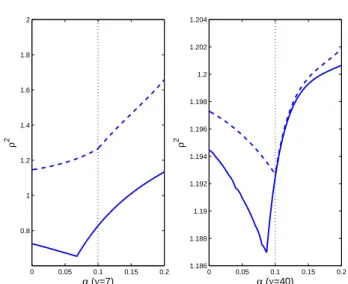
Example 2 (continued) We consider the following

fam-ily of 5-point designs: ξ(α) = (α, α+(1−2α)/4, α+(1−

0 0.1 0.2 0.3 0.4 0.5 0.6 0.7 0.8 0.9 1 0 0.2 0.4 0.6 0.8 1 1.2 x ρ 2(x)

Fig. 6 Kriging variance (normalized) and bounds for the 5-point minimax-optimal design with, in solid lines from top to bottom, ¯

ρ(x) given by (24) and the exact (normalized) kriging variance ρ2_{(x); the values of ρ}2

0(x) and of its upper bound ¯ρ0(x) (22) are

indicated in dotted lines.

0 0.1 0.2 0.3 0.4 0.5 0.6 0.7 0.8 0.9 1 0 0.2 0.4 0.6 0.8 1 1.2 x ρ 2(x)

Fig. 7 Kriging variance (normalized) and bounds for the 5-point maximin-optimal design with, in solid lines from top to bottom, ¯

ρ(x) given by (24) and the exact (normalized) kriging variance ρ2_{(x); the values of ρ}2

0(x) and of its upper bound ¯ρ0(x) (22) are

indicated in dotted lines.

2α)/2, α + 3(1 − 2α)/4, 1 − α), which includes ξ∗ M m(for

α = 0) and ξ∗

mM (for α = 0.1). The correlation function

is C(t) = exp(−ν t). Fig. 8 presents maxx∈Xρ2(x) and

¯

ρ2 _{given by (25) as functions of α in the strong (left,}

ν = 7) and weak (right, ν = 40) correlation cases.

Al-though the curves do not reach their minimum value for the same α, they indicate the same preference between

ξ∗

0 0.05 0.1 0.15 0.2 0.8 1 1.2 1.4 1.6 1.8 2 α (ν=7) ρ 2 0 0.05 0.1 0.15 0.2 1.186 1.188 1.19 1.192 1.194 1.196 1.198 1.2 1.202 1.204 α (ν=40) ρ 2

Fig. 8 maxx∈Xρ2(x) (solid line) and ¯ρ2 (25) (dashed line) as functions of α for the design ξ(α) when ν = 7 (left) and ν = 40 (right); the maximin-optimal design corresponds to α = 0, the minimax-optimal design to α = 0.1 (dotted vertical line).

4.3 Maximum-Entropy Sampling

Suppose that X is discretized into the finite set XN

with N points. Consider yN, the vector formed by Y (x)

for x ∈ XN, and y(ξ), the vector obtained for x ∈ ξ.

For any random y with p.d.f. ϕ(·) denote ent(y) the (Shannon) entropy of ϕ, see (11). Then, from a classical theorem in information theory (see, e.g., Ash (1965, p. 239)),

ent(yN) = ent(yξ) + ent(yN \ξ|yξ) (26)

where yN \ξ denotes the vector formed by Y (x) for x ∈

XN \ ξ and ent(y|w), the conditional entropy, is the

expectation with respect to w of the entropy of the conditional p.d.f. ϕ(y|w), that is,

ent(y|w) = − Z ϕ(w) µZ ϕ(y|w) log[ϕ(y|w)] dy ¶ dw .

The argumentation in (Shewry and Wynn, 1987) is as follows: since ent(yN) in (26) is fixed, the natural

ob-jective of minimizing ent(yN \ξ|yξ) can be fulfilled by

maximizing ent(yξ). When Z(x) in (16) is Gaussian,

ent(yξ) = (1/2) log det(C) + (n/2)[1 + log(2π)], and

Maximum-Entropy-Sampling corresponds to maximiz-ing det(C), which is called D-optimal design (by anal-ogy with optimum design in a parametric setting). One can refer to (Wynn, 2004) for further developments.

Johnson et al (1990) show that a maximin-optimal design is asymptotically D-optimal when the correla-tion funccorrela-tion has the form Ck_{(·) with k tending to}

infin-ity (i.e., it tends to be D-optimal for weak correlations). We have considered in Sect. 3.3 the design criterion (to be maximized) given by a plug-in kernel estimator ˆHn α

of the distribution of the xi, see (13) and (12). When

α = 2, the maximization of ˆHn α is equivalent to the minimization of φ(ξ) =X i,j K µ xi− xj hn ¶ .

A natural choice in the case of prediction by kriging is K[(u − v)/hn] = C(ku − vk), which yields φ(ξ) =

P

i,j{C}ij. Since C has all its diagonal elements equal

to 1, its determinant is maximum when the off-diagonal elements are zero, that is when φ(ξ) = n. Also note that 1 − (n − 1)CM m≤ λmin(C) ≤ φ(ξ)

n =

1>_C1

n

≤ λmax(C) ≤ 1 + (n − 1)CM m.

The upper bound on λmax(C) is derived in Appendix

C. The lower bound is obtained from λmin(C) ≥ t −

s√n − 1 with t = tr(C)/n and s2_{= tr(C}2_{)/n − t}2_{, see}

Wolkowicz and Styan (1980). Since {C}ij = {C}ji ≤

CM m for all i 6= j, we get tr(C) = n and tr(C2) ≤

n[1 + (n − 1)C2

M m] which gives the lower bound above.

Note that bounds on λmin(C) have been derived in

the framework of interpolation with radial basis func-tions, see Narcowich (1991); Ball (1992); Sun (1992) for lower bounds and Schaback (1994) for upper bounds. A maximin-distance design minimizes CM m and thus

minimizes the upper bound above on φ(ξ).

5 Design for estimating covariance parameters We now consider the case where the covariance C used for kriging (Sect. 4.1) depends upon unknown parame-ters ν that need to be estimated (by Maximum Likeli-hood) from the dataset y(ξ).

5.1 The Fisher Information matrix

Under this assumption, a first step towards good diction of the spatial random field may be the pre-cise estimation of both sets of parameters β and ν. The information on them is contained in the so-called Fisher information matrix, which can be derived ex-plicitly when the process Z(·) is Gaussian. In this case the (un-normalized) information matrix for β and θ = (σ2

Z, ν>)> is block diagonal. Denoting Cθ= σZ2Cν, we

get Mβ,θ(ξ; β, θ) = µ Mβ(ξ; θ) O O Mθ(ξ; θ) ¶ , (27)

where, for the model (16) with η(x, β) = r>_(x)β,

Mβ(ξ; θ) =

1

σ2

Z

with R = [r(x1), . . . , r(xn)]> and {Mθ(ξ; θ)}ij = 1 2tr ½ C−1 θ ∂Cθ ∂θi C−1 θ ∂Cθ ∂θj ¾ .

Since ˆY (x|ξ) does not depend on σZ and σZ2 only

in-tervenes as a multiplicative factor in the MSPE, see Sect. 4.1, we are only interested in the precision of the estimation of β and ν. Note that

Mθ(ξ; θ) = µ n/(2σ4 Z) z>ν(ξ; θ) zν(ξ; θ) Mν(ξ; ν) ¶ with {zν(ξ; θ)}i = 1 2σ2 Z tr µ C−1 ν ∂Cν ∂νi ¶ {Mν(ξ; ν)}ij = 1 2tr ½ C−1 ν ∂Cν ∂νi C−1 ν ∂Cν ∂νj ¾ . Denote M−1 θ (ξ; θ) = µ a(ξ; θ) b> ν(ξ; θ) bν(ξ; θ) Aν(ξ; ν) ¶ .

The block of Aν(ξ; ν) then characterizes the precision

of the estimation of ν (note that Aν(ξ; ν) = [Mν(ξ; ν)−

2σ4

Zzν(ξ; θ)z>ν(ξ; θ)/n]−1does not depend on σZ). The

matrix Aν(ξ; ν) is often replaced by M−1ν (ξ; ν) and

Mβ,θ(ξ; β, θ) by Mβ,ν(ξ; β, θ) = µ Mβ(ξ; θ) O O Mν(ξ; ν) ¶ ,

which corresponds to the case when σZ is known. This

can sometimes be justified from estimability consider-ations concerning the random-field parameters σZ and

ν. Indeed, under the infill design framework (i.e., when

the design space is compact) typically not all parame-ters are estimable, only some of them, or suitable func-tions of them, being micro-ergodic, see e.g. Stein (1999); Zhang and Zimmerman (2005). In that case, a reparame-trization can be used, see e.g. Zhu and Zhang (2006), and one may sometimes set σZ to an arbitrary value.

When both σZ and ν are estimable, there is usually no

big difference between Aν(ξ; ν) and M−1ν (ξ; ν).

Following traditional optimal design theory, see, e.g., Fedorov (1972), it is common to choose designs that maximize a scalar function of Mβ,ν(ξ; β, θ), such as its

determinant (D-optimality). M¨uller and Stehl´ık (2010) have suggested to maximize a compound criterion with weighing factor α,

ΦD[ξ|α] = (det[Mβ(ξ; θ)])α (det[Mν(ξ; ν)])1−α . (28)

Some theoretical results for special situations showing that α → 1 leads to space-filling have been recently given in (Kiseˇl´ak and Stehl´ık, 2008), (Zagoraiou and Antognini, 2009) and (Dette et al, 2008); Irvine et al (2007) motivate the use of designs with clusters of points.

5.2 The modified kriging variance

G-optimal designs based on the (normalized) kriging variance (19) are space filling (see, e.g., van Groeni-gen (2000)); however, they do not reflect the resulting additional uncertainty due to the estimation of the co-variance parameters. We thus require an updated de-sign criterion that takes that uncertainty into account. Even if this effect is asymptotically negligible, see Put-ter and Young (2001), its impact in finite samples may be decisive, see M¨uller et al (2010).

Various proposals have been made to correct the kriging variance for the additional uncertainty due to the estimation of ν. One approach, based on Monte-Carlo sampling from the asymptotic distribution of the estimated parameters ˆνn_{, is proposed in (Nagy et al,}

2007). Similarly, Sj¨ostedt-De-Luna and Young (2003) and den Hertog et al (2006) have employed bootstrap-ping techniques for assessing the effect. Harville and Jeske (1992) use a first-order expansion of the krig-ing variance for ˆνn _{around its true value, see also Abt}

(1999) for more precise developments and Zimmerman and Cressie (1992) for a discussion and examples. This has the advantage that we can obtain an explicit correc-tion term to augment the (normalized) kriging variance, which gives the approximation

˜ ρ2 ξ(x, ν) = ρ2ξ(x, ν) +tr ½ M−1ν (ξ; ν) ∂v> ν(x) ∂ν Cν(ν) ∂vν(x) ∂ν> ¾ , (29)

with vν(x) given by (18) (note that ˜ρ2ξ(xi, ν) = 0 for all

i). Consequently, Zimmerman (2006) constructs designs

by minimizing ˜ φG(ξ) = max x∈Xρ˜ 2 ξ(x, ν) (30)

for some nominal ν, which he terms EK-(empirical kri-ging-)optimality (see also Zhu and Stein (2005) for a similar criterion). The objective here is to take the dual effect of the design into account (obtaining ac-curate predictions at unsampled sites and improving the accuracy of the estimation of the covariance pa-rameters, those two objectives being generally conflict-ing) through the formulation of a single criterion. One should notice that ˜ρ2

ξ(x, ν) may seriously overestimate

the MSPE at x when the correlation is excessively weak. Indeed, for very weak correlation the BLUP (17) ap-proximately equals r>_{(x) ˆβ excepted in the}

neighbor-hood of the xidue to the interpolating property ˆY (xi|ξ)

= Y (xi) for all i; v(x) then shows rapide variations in

the neighborhood of the xi and k∂v(x)/∂νk may

be-come very large. In that case, one may add a nugget ef-fect to the model and replace (16) by Y (x) = η(x, β) +