HAL Id: hal-03215487
https://hal.archives-ouvertes.fr/hal-03215487
Submitted on 3 May 2021
HAL is a multi-disciplinary open access
archive for the deposit and dissemination of
sci-entific research documents, whether they are
pub-lished or not. The documents may come from
teaching and research institutions in France or
abroad, or from public or private research centers.
L’archive ouverte pluridisciplinaire HAL, est
destinée au dépôt et à la diffusion de documents
scientifiques de niveau recherche, publiés ou non,
émanant des établissements d’enseignement et de
recherche français ou étrangers, des laboratoires
publics ou privés.
Mathieu Vrac, Thomas Noël, Robert Vautard
To cite this version:
Mathieu Vrac, Thomas Noël, Robert Vautard. Bias correction of precipitation through Singularity
Stochastic Removal: Because occurrences matter. Journal of Geophysical Research: Atmospheres,
American Geophysical Union, 2016, 121 (10), pp.5237-5258. �10.1002/2015JD024511�. �hal-03215487�
Bias correction of precipitation through Singularity Stochastic
Removal: Because occurrences matter
Mathieu Vrac1, Thomas Noël1, and Robert Vautard1
1Laboratoire des Sciences du Climat et de l’Environnement (LSCE-IPSL, CNRS/CEA/UVSQ), Centre d’Etudes de Saclay, Orme des Merisiers, Gif-sur-Yvette, France
Abstract
This study focuses on how the treatment of the rainfall occurrences in bias correction (BC) contexts may affect the resulting precipitation, both in terms of occurrence and intensity. Threemethodologies are compared—the “direct approach” (DA), the “Threshold Adaptation” approach (TA), and the “Positive Approach” (Pos)—as well as a method called “Singularity Stochastic Removal” (SSR) specifically developed for precipitation, all based on the same adjustment technique. Unlike the three other models, SSR allows dealing in the same way with the situations where the precipitation model has too many wet days or not with respect to the reference data. SSR also avoids separating the correction of the occurrence from that of the intensity, which constitutes a flexible tool. First, the four approaches are applied to a historical regional climate model precipitation run. Evaluations are realized through occurrence- and intensity-related criteria. Although SSR, DA, and Pos may be close to each other depending on the criterion, in general, SSR provides the best results when all criteria are accounted for. This is even more true when the classical assumption that “the model precipitation had too many wet days” does not hold. The BC methods are also intercompared over the 2071–2100 period. The different BC methods are in agreement with previous studies, with relatively equivalent evolutions from 1976–2005 to 2071–2100, although nuances are present from one BC method to another. As a global conclusion, the SSR method for precipitation is a good compromise to correct both occurrences and intensities.
1. Introduction
Bias correction or bias adjustment of global (GCMs) or regional climate models (RCMs) has become a com-mon and quasi-mandatory step before using those model simulations in impact studies context. Indeed, most of the “raw” climate model outputs suffer from biases with respect to reality (or at least to what is measured) in the sense that their statistical distribution and properties differ from those of the observations [e.g., Vrac and Friederichs, 2015]. Eden et al. [2012] distinguished three sources for such precipitation biases in GCMs: the large-scale atmospheric conditions differ from observed ones (type 1 error), internal variability of a freely evolving GCM is different from the real world (type 2 error), and convection and precipitation parame-terizations can be deficient and the model orography differs from the real one (type 3 error). Type 2 errors can be reduced to some extent by temporal averaging, and the correction of type 1 errors is arguable [Eden et al., 2012]. However, it is often necessary to remove type 3 biases before further studies, e.g., to properly represent threshold exceedances in impacts estimation. The goal is then to adjust or correct model outputs by trans-forming them in order to have adjusted values—with statistical properties/distribution similar to those of observations used as reference—that can be employed as input into impact (or more generally subsequent) models.
Various methodologies have been developed over the last decades to perform such a task, from very simplis-tic methods, such as the so-called “delta” method [e.g., Hay et al., 2000; Lenderink et al., 2007], only correcting the statistical mean of the simulations, to more sophisticated ones, for example based on stochastic mod-elling applied to nudged RCMs (such as in Wong et al. [2014] and Eden et al. [2015]). The most popular and commonly applied bias correction (BC) approach is based on the quantile-mapping technique [Panofsky and
Brier, 1958; Haddad and Rosenfeld, 1997; Wood et al., 2004; Déqué, 2007; Piani et al., 2010a; Gudmundsson et al.,
2012], mapping a model outptut x with cumulative distribution function (CDF) FX, to an observation y, with CDF FY, through a function h, such that the two distributions are equivalent [Piani et al., 2010b]:
y = h(x) such that FY(y) = FX(x). (1)
RESEARCH ARTICLE
10.1002/2015JD024511
Key Points:
• Study on how the treatment of rain occurrence in bias correction affects occurrence and intensity
• Bias correction method (SSR) specific to precipitation
• Global conclusion: the SSR method is a good compromise to correct both occurrences and intensities
Correspondence to:
M. Vrac,
mathieu.vrac@lsce.ipsl.fr
Citation:
Vrac, M., T. Noël, and R. Vautard (2016), Bias correction of precipitation through Singularity Stochastic Removal: Because occurrences matter, J. Geophys. Res. Atmos., 121, 5237–5258, doi:10.1002/2015JD024511.
Received 18 NOV 2015 Accepted 12 APR 2016
Accepted article online 3 MAY 2016 Published online 19 MAY 2016
©2016. American Geophysical Union. All Rights Reserved.
Although h can be modeled through either parametric or nonparametric distributions and regression-like transformations [e.g., Gudmundsson et al., 2012], the so-called “Empirical Quantile Mapping” (EQM)—a distribution-derived nonparametric approach [e.g., Déqué, 2007]—is one of the most commonly applied methods, directly deriving the corrected value y from the modeled value x:
y = F−1
Y (FX(x)), (2)
where F−1is the inverse function of the CDF F, both modeled nonparametrically.
Bias correction models are sometimes applied as statistical downscaling tools [Vrac et al., 2012; Vaittinada
Ayar et al., 2015]. In such a case, the spatial autocorrelation of the corrected fields may likely be overly
smooth and not match observations [e.g., Maraun, 2013]. Nevertheless, various differences may be considered between statistical downscaling models (SDMs) and the BC model. Both types of models need observed data (for reference in BC or local-scale data in SDM). However, one major point of view is certainly that most of the SDMs are in a so-called “perfect-prog” context [e.g., Maraun et al., 2010]. This means that those statistical models have first to be calibrated (i.e., trained) based on large-scale observations that usually are reanalyses. In contrast, BC models are generally in a “Model Output Statistics” (MOS) context [e.g, Wong et al., 2014;
Vaittinada Ayar et al., 2015] where they are directly “calibrated” to link (and therefore correct) the modeled
data, e.g., from GCMs or RCMs, to (respectively, with respect to) the reference data. Consequently, bias correc-tion is climate model dependent, in the sense that two climate models will need two different BC calibracorrec-tions to have corrected values with statistical properties/distribution similar to those of observations used as reference. As SDMs are generally perfect-prog models, the same calibration based on reanalyses is applied to any climate models, assuming therefore that the large-scale predictors are all unbiased with respect to reanalysis data. Of course, as it cannot always be considered as true, some approaches try to bias correct GCM simulations before incorporating them into statistical downscaling models [e.g., Wood et al., 2004; Maurer, 2007; Ahmeda et al., 2013].
Moreover, one classical feature of BC methods is that only one predictor is usually employed: the modeled vari-able of interest. In other words, if one wants to correct the output of temperature of a given RCM for example, only this variable is used to make it resemble the (generally observed) reference data set of temperature. Some BC models tried to overcome this constraint by adding other covariates in different ways, such as in
Kallache et al. [2011], Wong et al. [2014], or Eden et al. [2015]. The use of multiple predictors (i.e., not only the
variable of interest) is, however, a quite common and required approach for SDMs, trying to incorporate more atmospheric, dynamical, etc., information than the single large-scale variable to be downscaled.
Traditionally, bias correction is applied in a univariate context, i.e., separately for each location and variable of interest. This may of course be a problem when the obtained corrected data are used as input in impact models needing, for example, input data with some spatial coherency and dependence among variables. The latter could have been destroyed by the application of univariate BC models. That is why, recently, different methodological improvements have been made in terms of multidimensional statistical properties to be pre-served. For example, some BC models have been proposed for bivariate (i.e., two climate variables) correction [Piani and Haerter, 2012], for correction accounting for intervariable (i.e., multivariate) or spatial dependences [Mao et al., 2015], accounting for both intervariable and temporal dependences [Mehrotra and Sharma, 2015], or accounting for both intervariable, spatial and temporal properties [Vrac and Friederichs, 2015].
Nevertheless, if those approaches are valuable contributions to improve the quality of the corrected data and their various dependences, all climate variables cannot be corrected in the same way due to specificities and constraints. This is the case of the variable precipitation. Many (if not all of the) climate variables have been corrected for many applications including temperature or extreme temperature [Déqué, 2007; Christensen
et al., 2008; Lavaysse et al., 2012, among many others], precipitation or extreme precipitation [e.g., Christensen et al., 2008; Kallache et al., 2011; Themeßl et al., 2011; Lavaysse et al., 2012; Wong et al., 2014], wind speed or
zonal and meridional wind components [e.g., Michelangeli et al., 2009; Colette et al., 2012; Vrac et al., 2012], and some more unusual climate, atmospheric, or environmental parameters such as solar radiation and insolation [Oettli et al., 2011], three-dimensional relative humidity and wind components [Colette et al., 2012], or hydrocli-matic descriptors of fish habitats such as monthly river flows and temperature percentiles [Tisseuil et al., 2012]. However, bias correction of precipitation at the daily or subdaily time step is peculiar due to the large number of no-precipitation events (i.e., zero values) that are difficult to correct properly while their presence/absence and the associated persistence are important features necessary in many disciplines such as agriculture,
hydrology, etc. Indeed, rainfall occurrences play a central role in various applications or models. For example, they are used as a conditioning variable in various stochastic models (i.e., its value is used as a covariate to condition stochastic models), such as for daily solar irradiance simulations [e.g., Hansen, 1999; Garcia y Garcia
and Hoogenboom, 2005] or to condition some parameterizations, e.g., in process-based snowmelt modelling
where occurrence can be used as a surrogate for cloud cover [Walter et al., 2005]. Consequently, a reliable simulation (or correction) of rainfall occurrence is therefore a prerequisite to drive and apply correctly sub-sequent models. More generally, disposing of “clean” (in the sense “statistically debiased”) precipitation data is a major requisite to lead relevant climate-related analyses, both in retrospective (i.e., past) or prospective (i.e., future) climate contexts.
As mentioned in Argüeso et al. [2013], most of the BC methods “assume that the model produces the same or a higher number of rain days, independently from how these are defined.” In other words, if the climate model precipitation to be corrected has too many dry days (i.e., not enough wet days), the bias correction method might not be able to correct realistically the daily intensity. When the model respects the tradi-tional assumption of “too many wet days”, a relatively common approach consists in applying a “threshold adaptation” procedure to define a threshold t for which model data below t are put to zero [e.g., Schmidli et al., 2006; Ines and Hansen, 2006; Lavaysse et al., 2012]. This threshold is chosen such that the frequency of days with model precipitation> t is the same as the frequency of rainy days in the reference (observed) precipitation data set. After this thresholding, only the positive values are corrected. Other approaches are also possible. For example, in the context of an RCM forced by reanalysis data, Mao et al. [2015] only corrected partially the positive intensities of precipitation, without correcting the dry event frequency. Hereafter, this approach will be referred to as the “Positive correction” approach, implying that model dry days are not corrected. Another method to deal with the precipitation correction consists in applying a BC model directly on the whole time series including both dry days and rainy days, i.e., without separating the correction methodology into occur-rence and intensity (Piani et al. [2010a], Vrac et al. [2012], and Vigaud et al. [2013], among others). Hereafter, this approach will be referred to as the “Direct” approach.
However, when the model has too few wet days, the direct approach should generate a wet precipitation bias, the “positive” correction yields a dry precipitation bias and the threshold adaptation strategy cannot work by construction. Themeßl et al. [2012] suggested to add more rainy days through the so-called “frequency adaptation,” basically consisting of a threshold adaptation but applied the other way around, i.e., with the threshold defined in the world of the observations. Based on this threshold, a fraction of randomly selected dry days is transformed into wet days to retrieve the correct dry-day frequency, and an adjustment is performed on the positive values. In the classical case of too many wet days in the model, however, this approach is not applicable directly and one has to apply another choice, i.e., a direct approach correction, or a classical threshold adaptation one. In other words, in order to consider all situations, subcases have then generally to be made: one correction approach to be applied when the model has too many wet days, another approach in the other case.
Therefore, the goal of this study is to investigate a bias correction methodology that first allows removing subcases in dealing with both situations in the same way and also avoids separating the correction of the occurrence from that of the intensity of precipitation, which constitutes therefore a more flexible tool. As in
Cannon et al. [2015], this is achieved by transforming all model and reference dry days into small but positive
values before applying an adjustment method and thresholding back. Moreover, this paper focuses on how the treatment of the rainfall occurrences may affect the corrected precipitation, not only in terms of occurrence properties but also in terms of intensity (including dry event or not), in comparing the different methodologies mentioned above, as well as this flexible approach.
This paper is organized as follows: Section 2 presents the data used in this study and the evaluation procedure. The investigated BC method for precipitation is detailed in section 3, and the different compared methods are also listed. The results are given in section 4, while section 5 summarizes the conclusions and provides some discussions.
2. Data and Evaluation Procedure
2.1. Model and Reference Data
The model data to be corrected in this study are daily precipitation outputs over the European domain of the Coordinated Regional Climate Downscaling Experiment [CORDEX, see Giorgi et al., 2009; Jacob et al., 2014]
from the “Weather Research and Forecasting” (WRF) regional climate model (RCM) developed by the National Center for Atmospheric Research [Skamarock et al., 2008]. WRF was forced by a so-called “historical” 1950–2005 run [Intergovernmental Panel on Climate Change (IPCC), 2013] of the “Institut Pierre Simon Laplace” (IPSL) global climate model [Marti et al., 2010; Dufresne et al., 2013]. The obtained downscaled simulations (hereafter referred to as WRF-IPSL simulations) at a 0.11∘ horizontal resolution are therefore part of the EURO-CORDEX international initiative [Kotlarski et al., 2014; Jacob et al., 2014]. The model chain is described in Menut et al. [2012] and Vautard et al. [2013]. The ability of the model as well as other EURO-CORDEX RCMs to simulate the European climate has been described in a few other studies [Kotlarski et al., 2014; Katragkou
et al., 2014; García-Díez et al., 2015]. Note that two other RCM/GCM combinations have also been considered:
the COSMO - Climate Limited-area Modelling RCM version 4 [CCLM4, Rockel et al., 2008] forced by the Centre National de Recherches Météorologiques (CNRM) [Voldoire et al., 2013] GCM and the the Rossby Centre regional Atmospheric model [RCA4, Samuelsson et al., 2011] forced by the IPSL GCM. However, for those runs, the quality of the results in terms of correction were equivalent to those presented later in section 4 for the WRF-IPSL results and are therefore not shown in this article.
The precipitation time series used as reference in this study come from the ENSEMBLE project gridded data set [EOBS, Haylock et al., 2008] obtained through an interpolation procedure from “European Climate Assessment and Dataset” (ECA&D) time series at meteorological stations [Klok and Klein Tank, 2009]. The EOBS version used in this study is the version 10 (released date: April 2014) and covers inland Europe on a rotated grid with a spatial resolution of 0.22∘ from 1950 to 2013 at a daily time step.
In order to have a common spatial resolution between the RCM simulations and the EOBS reference times series, the RCM simulations have first been regridded by aggregating grid cells by four, to obtain model data at a 0.22∘ spatial resolution (rotated grid as specified for the simulations), matching exactly that of EOBS. For each regridded RCM grid point, the associate EOBS grid point is then taken as the reference for correction. However, other choices could have been made, for example, based on location representativeness of the GCM gridcells [Maraun and Widmann, 2015].
Moreover, in some studies, before proceeding to the bias correction, a thresholding is classically applied to rainfall data to put small precipitation values at zero. A wide panel of thresholds is used in the literature: for example, 0 mm in Semenov et al. [1998], 0.5 mm in Ambrosino et al. [2014], 1 mm in Schmidli et al. [2007] or
Vaittinada Ayar et al. [2015], or 5 mm in Bouvier et al. [2003]. In the following, in order to keep the properties of
the reference and model data as untouched as possible before correction, no threshold is used (i.e., equivalent to a 0 mm threshold). However, thresholds of 0.5 mm and 1 mm have been tested and did not change the conclusions presented later. Therefore, the associated results are not mentioned any more.
2.2. Historical Evaluations and Future Comparisons
To evaluate the quality of the BC methods in a historical context, the bias-corrected data have to be compared to the EOBS reference data. To do so in a calibration/evaluation framework, the calibration of the BC meth-ods is performed over 1979–1988, while the corrected data are generated and evaluated over 1989–2005. Unlike an evaluation of correction performed directly on the calibration period (i.e., correction and evaluation period = calibration period), this cross-validation framework allows characterizing the quality of corrections for data on which they have not been directly calibrated. This is usually more informative of the behavior of the methods as applied in a climate change context. In a “projection = calibration” framework, some approaches, like the “Direct approach” or the “Threshold adaptation” in some cases, may artificially appear very close to the reference data while they are not in a cross-validation framework that tests more the applicability and efficiency of the methods to new data.
To evaluate how the BC methods differ in their results in a climate change context, they are calibrated over the 1971–2005 period and applied to the 1971–2100 time period and compared through the 30 year 2071–2100 time period.
3. Bias Correcting Precipitation: Occurrence and Intensity
3.1. The “Singularity Stochastic Removal” Approach
The investigated approach to deal with correction of precipitation occurrences is based on replacements of the 0 values in the model and observational data by randomly selected extremely small but nonzero values. This basic approach is similar to that utilized in Zhang et al. [2009] in a context of temperature
Figure 1. Schematic view of how the “Singularity Stochastic Removal” (SSR) proceeds. For simplification, this is
illustrated for the case where the model data for calibration are also used for projection.P0(M)is the probability of null precipitation in the model, whileP0(ref ) is the probability in the reference data; th is the selected threshold (th is lower than the minimum observed and modelled strictly positive values). (a) The grey line corresponds to the CDF of the model simulations and the black line to the CDF of the reference data. (b) Each value lower than th is replaced by a randomly simulated value following a uniform distribution in]0,th[. (c) The adjustment is performed on the newly obtained data sets (in this “projection = calibration” case, the adjusted modelled data will have a CDF corresponding to that of the reference data). (d) All values below th are set to 0.P0(BC) is the probability of null precipitation values in the bias-corrected data.
percentile indices and by Cannon et al. [2015] for quantile-mapping bias correction of precipitation. The procedure—presented in a schematic way in Figure 1—is the following:
1. Determine a positive precipitation threshold th such that all model and observational strictly positive data are higher than th. For example, th can be defined as the minimum of all strictly positive model and reference data.
2. Then, for each null value (in the model and the observations), simulate a value v according to a random vari-able V distributed uniformly between 0 and th, i.e., V ∼ U]0,th[, and replace each null value by a simulated v. Hence, new time series are generated where data higher than th (i.e., the strictly positive precipitation values) are untouched and where previously zero values have been replaced by simulated data in ]0, th[. 3. Apply an adjustment method to the newly generated times series.
4. The bias-corrected data lower than th are set to 0.
This approach, hereafter referred to as “Singularity Stochastic Removal” (SSR), allows dealing in the same way with cases where the proportion of dry days in the model is higher than that in the reference data and in the inverse cases where the proportion of dry days in the model is lower than that in the reference data. This is performed by step (2) of the procedure that removes the singularity brought by the zeroes in the time series. Therefore, this allows applying most of the adjustment methods without considering zeroes anymore. It also avoids separating the correction of the occurrence from that of the intensity of precipitation by correcting all at once and performing a thresholding (to generate dry days) after a global correction. In the following, the parameter th is set to 10−8mm/s (corresponding to 8.64 × 10⁻⁴mm/day). Higher and lower values of th have been tested, but all gave relatively equivalent results to those presented in section 4 and are then not shown.
3.2. Intercomparison
In order to evaluate the SSR approach for correcting precipitation and more specifically precipitation occurrences, several other approaches—commonly used in the scientific literature—are also tested. In total, four different methods are tested:
1. Positive correction. No correction of the model occurrences; only the intensity is bias corrected [Mao et al., 2015].
2. Threshold adaptation. Find a threshold thmodelfor the model data such that
Pr(Obs = 0) = Pr(Mod≤ thmodel). (3)
All model data lower than or equal to thmodelare put to 0, and an adjustment method is applied only to model data higher than thmodelbased on observational data strictly positive. If some bias-corrected data are positive but lower than thmodel, they are put to 0 [e.g., Schmidli et al., 2006; Ines and Hansen, 2006; Lavaysse
et al., 2012].
3. Direct approach. The adjustment method is applied directly to all model data, including zeroes (Piani et al. [2010a], Vrac et al. [2012], and Vigaud et al. [2013], among others).
4. The Singularity Stochastic Removal approach.
In practice, the Threshold adaptation approach may be difficult to apply. Indeed, this method is applicable only when the proportion of dry days in the model data is lower than the proportion of dry days in the refer-ence data. If this is not the case, the grid point associated with such a time series is not treated, i.e., the bias correction is not performed with the TA approach but only with the other approaches.
In the following, only one adjustment method for precipitation intensity is applied: the “Cumulative Distribution Funtion-transform” (CDF-t) approach. Indeed, although other methods could have been included in this study, the influence of the adjustment method for intensity on the four tested approaches for dealing with occurrences is beyond the scope of the present article. Moreover, it is strongly expected that the results and the ranking of the methods for occurrences will be equivalent with other methods for intensity correction. Hence, only CDF-t is used here. In the following, the different BC strategies for precipitation (Positive correction,
Threshold adaptation, Direct approach, and Singularity Stochastic Removal, hereafter referred to as Pos, TA, DA,
and SSR, respectively) are associated with the precipitation-specific CDF-t adjustment method and are applied to daily precipitation data on a monthly basis, i.e., separately for each of the 12 calendar months.
3.3. Short Reminder on the CDF-t Approach and Specific Formulation for Precipitation
The “Cumulative Distribution Function-transform” (CDF-t) approach was initially developed for wind speed bias correction and downscaling [Michelangeli et al., 2009] and has then also been applied to temperature or precipitation [Kallache et al., 2011; Vrac et al., 2012; Lavaysse et al., 2012; Vigaud et al., 2013; Vautard et al., 2013], as well as to other diverse climate, atmospheric or environmental parameters such as solar radiation and insolation [Oettli et al., 2011], three-dimensional relative humidity and wind components [Colette et al., 2012], or hydroclimatic descriptors of fish habitats such as monthly river flows and temperature percentiles [Tisseuil et al., 2012].
CDF-t can be considered as a variant of the empirical quantile-mapping method. It first estimates the CDF FYp and FXpof the random variables Y and X —representing, respectively, the reference and model data—over a projection time period (either future or evaluation time period) before applying a distribution-derived quan-tile mapping as defined in (2). The CDF FXpof the model data can be directly estimated from the data to be corrected in the projection period. For the CDF FYp, the modeling is based on the assumption that a mathematical transformation T allows going from FXto FYin the calibration period, i.e.,
T[FX(z)] = FY(z) (4)
for all z in the domain of X and Y. It is also assumed that T is valid in the projection period:
T[FXp(z)] = FYp(z). (5)
When replacing z by F−1
X (u) in (4), with u being a probability value (i.e., in [0, 1]), it can derive a simple definition for T through T(u) = FY [ F−1 X (u) ] . (6)
Table 1. Summary of the Utilized Evaluation Criteria
Acronym Long Name Unit
BP(wet) Bias in annual wet day probability – 𝜌wet Spearman correlation of the monthly wet day proba seasonal cycle –
BPerswet Bias in mean wet persistence days BPersdry Bias in mean dry persistence days SB Yearly average of the mean seasonal biases mm/day 𝜌SC Spearman correlation between the monthly intensity seasonal cycle and that of EOBS –
Rvar(%) Ratio of BC variances over that of EOBS % R]0,1] Mean ratio (BC/EOBS) of the number of values in]0, 1] %
B10yRL Bias in 10 year return level mm
%>Q95 % of BC values>than the seasonal 95th EOBS percentile in the projection period %
When combining this with (5), an estimation of FYpis obtained:
FYp(z) = FY { F−1 X [FXp(z)] } . (7)
Based on FXpand FYp, a distribution-based quantile mapping is applied as in (2). Hence, CDF-t performs a quantile-mapping technique based on the CDFs over the projection time period and therefore allows accounting for changes of CDF with respect to the calibration period. More details can be found in Vrac et al. [2012] and Vrac and Friederichs [2015].
When the model and reference data have CDFs very different from each other, the domain of FYpcan be the-oretically restricted [Michelangeli et al., 2009; Kallache et al., 2011]. In order to maximize this domain properly,
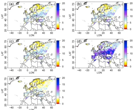
Figure 2. (a) Probabilites of wet days (all seasons together) in EOBS and differences of probabilities of wet days with
respect to EOBS percentages (i.e., proba from corrected data minus proba from EOBS) for (b) SSR, (c) Direct approach, (d) Threshold Adaptation approach, and (e) Positive approach. Note that the “Positive” approach corresponds here to take the wet or dry days of the model to be corrected, and thus Figure 2e corresponds to the differences of wet day probabilities in the climate model with respect to EOBS ones. (f ) The differences between the training and projection (i.e., evaluation) periods.
Figure 3. Spearman correlation between the seasonal cycle of wet days probabilities from EOBS and the seasonal cycle
from corrected data with (a) SSR, (b) Direct approach, (c) Threshold Adaptation approach, and (d) Positive approach. Note that the “Positive” approach corresponds here to take the wet or dry days of the model to be corrected, and thus Figure 3d corresponds to the Spearman correlation between the seasonal cycle of the model and that from EOBS. (e) The correlations between the training and projection (i.e., evaluation) periods.
for precipitation, the calibration model precipitation data {xi} are first “normalized” to {̃xi} in order to be in [0, Mref], where Mrefis the maximum value of the reference time series:̃xi= xi× Mref∕MCmod, where MCmodis the maximum value of the model time series over the calibration period. The same formulation (i.e., with the same parameters) is applied to normalize the model data {xp,i} over the projection time period into {̃xp,i}:
̃xp,i= xp,i× Mref∕MCmod. More details about the necessity and potential impacts of normalization can be found in Kallache et al. [2011].
4. Results
In order to understand the impact of the rainfall occurrence modelling on the bias-corrected precipitation, the evaluation of the corrections is performed according to two angles: (i) an evaluation based on the occurrences only and (ii) one based on the intensities (including or not the zeros). Hence, various criteria will be used to evaluate the different BC strategies. Those criteria are summarized in Table 1 and they will be described as they come along in the following sections.
4.1. Evaluation: Occurrences-Related Criteria
Figure 2 displays the wet day probabilities (all seasons together) in EOBS as well as the differences of wet day probabilities from each BC approach with respect to the EOBS probabilities (i.e., probabilities from the cor-rected data minus probabilities from EOBS, both over the projection period). While the positive BC approach (i.e., corresponding to the wet day probabilities of the RCM) in Figure 2e shows an overestimation of the wet days probabilities with respect to EOBS ones, the SSR approach as well as DA and the TA approach show rela-tively minor differences of wet day probabilities with respect to EOBS. We verified that this is also true for the training period (Figure 2f ) that shows very weak differences with the evaluation period.
This feature is also present in the seasonal cycles of the wet day probabilities when looking at point-wise Spearman correlations between the EOBS seasonal cycles of wet day probabilities and the equivalent seasonal cycles of each BC approach, in Figure 3 (note that by construction, the correlation of seasonal cycles of dry
Figure 4. (a) Mean wet persistence in winter (DJF) from EOBS data set and differences of mean wet persistence in winter
with respect to EOBS for (b) SSR, (c) DA, (d) TA approach, and (e) Positive approach. (f ) The differences between the training and projection (i.e., evaluation) periods. For Figures 4b–4f, upper values are censored at 10 days of differences for visualization purposes.
day probabilities would give the exact same results). To do so, for each grid point, wet day probability values have been averaged monthly across the time series and the correlation has been calculated based on those 12 values. Although the RCM (i.e., “positive” approach) provides here seasonal cycles with correlation to EOBS often higher than 0.5, it also generates seasonal cycles with correlations close to zero or even negative in many regions. SSR, DA, and the TA approach give results close to each other and in general present correlations higher than 0.5. However, for these three methods, it is interesting to note lower correlations over the central part of the domain, around France and Germany, and along the northern Norwegian coasts. Interestingly, this feature is also visible in the correlations between the training and projection (i.e., evaluation) periods. Lengths of wet or dry events are also important features that bias correction methods have to simulate cor-rectly in many applications. In that sense, the mean persistence is an informative criterion. It is calculated by first transforming the time series into wet (1) or dry (0) days. This allows defining periods (i.e., consecutive days) with only dry days (i.e., with at least one wet day before and one after the period) and periods with only wet days (i.e., at least one dry day before and one after). The duration (in days) of each wet or dry period was then calculated, and the mean dry or wet persistence corresponds to the average (per season) of those durations. The winter season is used (here and in the following) for illustration due to its representativeness of the quality of the results for the four seasons. Indeed, the results are usually relatively similar from one season to another for most of the bias-related criteria. However, for some criteria, results can of course differ for other seasons, for example, for summer where precipitation properties are different from those in winter. Therefore, summer-specific comments will be provided when needed to highlight the differences with win-ter results. Figure 4 shows the mean wet persistence in winwin-ter (December-January-February (DJF)) from EOBS data set in Figure 4a, as well as differences of mean wet persistence from the different BC approaches in Figures 4b–4e in winter with respect to EOBS. Once more, SSR (Figure 4b), DA (Figure 4c), and the TA approach (Figure 4d) are found to be the BC methods whose results are the closest to EOBS with small biases, while the positive approach in Figure 4e shows much larger positive biases, implying too long wet persistences.
Figure 5. Same as in Figure 4 but for dry persistence.
The EOBS training data (Figure 4f ) only have slight differences with respect to the EOBS evaluation data over the major part of the domain. This indicates that the mean wet persistence has not changed much from the training to the evaluation periods.
Figure 5 is the same as Figure 4 but for dry persistence. The positive approach mostly presents negative biases—between 0 and −5 days—indicating too short dry persistences. Although their spatially averaged mean dry persistence biases are around 0, SSR, DA, and TA display this time dry persistence biases with more
Table 2. Spatially and Yearly Averaged Values of the Occurrence- and Intensity-Related Criteria Calculated Only Over Grid
Points Where the Threshold Adaptation (TA) Method Worksa
Type of Criteria Criteria SSR DA TA Pos WRF Occurrence-related BP(wet) 1e−2 (1) 1e−2 (1) −1e−2 (1) −0.32 (4) −0.32 (4) 𝜌wet 0.6 (1) 0.66 (1) 0.6 (1) 0.36 (4) 0.36 (4) BPerswet −0.06 (1) −0.18 (2) −0.22 (3) 3.91 (4) 3.91 (4) BPersdry −0.46 (3) −0.36 (2) −0.25 (1) −1.63 (4) −1.63 (4) Averaged ranks 1.5 1.5 1.5 4 4 Intensity-related SB 0.15 (1) 0.17 (2) 0.17 (2) 1.73 (5) 0.73 (4) 𝜌SC 0.75 (1) 0.73 (1) 0.73 (1) 0.75 (1) 0.72 (1) Rvar(%) 176.2 (1) 198.2 (3) 196.4 (3) 182.4 (3) 163.1 (1) R]0,1] 108.31 (1) 81.05 (2) 78.48 (2) 149 (4) 425.3 (5) B10yRL 14.44 (2) 18.11 (3) 18.06 (3) 24.39 (5) 10.2 (1) %>Q95 5.55 (1) 5.48 (1) 5.47 (1) 11.23 (5) 4 (4) Averaged ranks 1.17 2 2 3.83 2.67 Global ranks
(occurrence and intensity) 1.3 1.8 1.8 3.9 3.2
aSee text for details as well as Table 1 for a summary. Note that by construction, the positive BC approach has the same
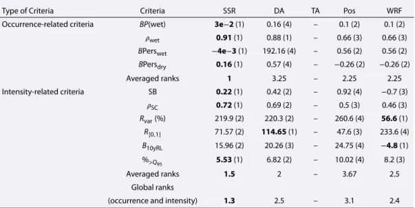
Table 3. Same as Table 2 but Only for the 783 Grid Points Where TA Is Not Applicable
Type of Criteria Criteria SSR DA TA Pos WRF Occurrence-related criteria BP(wet) 3e−2 (1) 0.16 (4) – 0.1 (2) 0.1 (2)
𝜌wet 0.91 (1) 0.88 (1) – 0.66 (3) 0.66 (3) BPerswet −4e−3 (1) 192.16 (4) – 0.56 (2) 0.56 (2) BPersdry 0.16 (1) 0.57 (4) – −0.26 (2) −0.26 (2) Averaged ranks 1 3.25 – 2.25 2.25 Intensity-related criteria SB 0.22 (1) 0.42 (2) – 0.92 (4) −0.7 (3) 𝜌SC 0.72 (1) 0.69 (2) – 0.5 (3) 0.46 (3) Rvar(%) 219.9 (2) 220.3 (2) – 260.6 (4) 56.6 (1) R]0,1] 71.57 (2) 114.65 (1) – 47.6 (3) 233.6 (4) B10yRL 15.96 (2) 20.26 (3) – 24.75 (4) −4.8 (1) %>Q 95 5.53 (1) 6.82 (2) – 10.02 (4) 8.2 (3) Averaged ranks 1.5 2 – 3.67 2.5 Global ranks
(occurrence and intensity) 1.3 2.5 – 3.1 2.4
variability—roughly between −3 and +2 days—from one grid point to another, with a southwest to northeast gradient, which is also visible for the training period in Figure 5f although less pronounced.
In order to have a more quantitative assessment of those visual evaluations, the upper halves of Tables 2 and 3 display the values of the previously mentioned biases or correlations that have been computed seasonally per grid point and then yearly and spatially averaged. The difference between those two tables is that Table 2 con-tains results obtained only for the grid points where the Threshold Adaptation approach is able to work—i.e., grid points where the proportion of wet days in the model is larger than or equal to that of the reference data—while Table 3 gives results only for the grid points where TA cannot work due to a lower propor-tion of wet days in the model than in the reference. Such locapropor-tions correspond to 783 grid points for our WRF-IPSL run (1586 for CCLM4-CNRM and 1429 for RCA4-IPSL). In each table and for each criterion, a rank-ing among the BC method is indicated in brackets: the lower the rankrank-ing, the better. Note that the criteria and ranks are also computed on the original (raw) RCM to assess the added value of the different BC strate-gies. Note also that ties in rank were awarded when the relative absolute difference between two values of a given criterion (i.e., 100 ×|value1 − value2|∕|value1|) is lower than 10%. This is, for example, the case for SSR and DA for𝜌wetin Table 2 (100 ×|0.66 − 0.6|∕|0.66| = 9% < 10%), but this is not the case for BPerswet (100 ×|−0.06 − (−0.18)|∕|−0.06| = 200% > 10%). In Table 2, although numerical values better allow us see-ing some differences between SSR, DA, and TA, as expected, they are relatively close to each other and the positive approach is much farther, ranking always 4 like the original RCM by construction. When averaging those ranks per BC method, the three methods SSR, DA, and TA obtain a 1.5 ranking, while Pos and WRF have 4. However, the conclusion is different when looking at Table 3, calculated for grid points where TA cannot be applied: here, SSR appears at rank 1 for all occurrence-related criteria. This time, Pos and the raw RCM are sec-ond but still farther with a rank 2.25 but still better than DA (rank 3.25). In other words, for grid points where TA cannot work, keeping the occurrences of the model (i.e., Positive approach) appears better than applying a direct approach, and SSR displays the best results in terms of occurrence-related criteria.
4.2. Evaluation: Intensity-Related Criteria
The occurrence biases can obviously affect the whole distribution of precipitation. Therefore, it is also nec-essary to evaluate the different BC methods in terms of precipitation intensity. The various intensity-related criteria used for that are also included in the second (i.e., lower) part of Tables 2 and 3. The results for the grid points where the Threshold Adaptation approach is able to work are first discussed.
A first classical indicator is the mean seasonal precipitation bias of the BC models with respect to EOBS. This is calculated by grid point for each of the four seasons (DJF, MAM (March-April-May), JJA (June-July-August), SON (September-October-November)), and then yearly and spatially averaged. The numerical results are given in the first line of the “Intensity-related criteria” part of Table 2. SSR, DA, and TA are still relatively close to each other with biases between 0.15 and 0.17 mm/day, and the positive approach has a larger mean seasonal
Figure 6. Spearman correlations (EOBS versus corrected data) of the seasonal cycles monthly intensities (calculated
without the null values) for each BC method: (a) SSR, (b) Direct approach, (c) TA approach, and (d) Positive approach. (e) The correlations between the training and projection (i.e., evaluation) periods.
bias of 1.73 mm/day. Interestingly, the raw original RCM shows a seasonal bias (0.73 mm/day) smaller than that of the positive approach, meaning that this latter strategy can degrade some basic statistical properties of the model to be corrected. However, this is not the case when calculating the Spearman correlations𝜌SC of the seasonal cycles of monthly intensities of each BC method with respect to the EOBS seasonal cycles (i.e., EOBS versus corrected data). The values of the spatially averaged correlations are given on line 𝜌SC of Table 2 and the maps in Figure 6. Those correlations were calculated based on strictly positive values, i.e., without the null values. Hence, the influences of biases in occurrence statistics are removed from this analysis. Results in including the null values are similar, although slightly degraded (not shown). Lower correlations appear over Spain for the four BC strategies, less visible although present in Figure 6e display-ing correlations between the traindisplay-ing and evaluation periods. Nevertheless, on average over the domain, all strategies remain satisfactory with a mean correlation around 0.74.
It is also interesting to look at the variability of the data, e.g., through the comparison of the variances from the BC models with respect to the EOBS data, both calculated without the null values. This is done in Figure 7 that displays, for winter, the EOBS precipitation variances in Figure 7a and the ratios (in %) of each bias-corrected data set to that of EOBS in Figures 7b–7e), where the closer the values to 100%, the better. In general, all models overestimate the variance. By comparison, we can see that the EOBS training data (Figure 7f ) have a variance closer to that of the evaluation period, even though strong underestimation of the variance is present in the north of the domain. When looking at the spatially and yearly averaged ratios of variances (line Rvarof Table 2), some differences appear between the different approaches: SSR and WRF have the ratios of variance the closest to 100% with 176.2 and 163.1%, respectively; DA and TA have a Rvararound 197% (i.e., almost twice the EOBS variance); and Pos of 182.4%. However, when including the null values to compute the variances (i.e., including the influences of biases in occurrence statistics), the Pos approach appears the farthest from the EOBS data with a strong overestimation of the variance (with Rvar= 244%), DA and TA still have a variance that is about twice that of EOBS (Rvarvalues around 210%), and SSR has still the variance ratio the closest to 100% (Rvar= 157%).
This variance ratio criterion, however, gives an evaluation of the variability over the whole distribution of the positive precipitation values. Therefore, to have a more precise understanding of the variability, it is also
Figure 7. (a) Variance of the EOBS time series in winter as well as ratios of variance (in %) in winter of each BC method
with respect to EOBS: (b) SSR, (c) DA, (d) TA, and (e) Pos. (f ) The variance ratio between the training and projection (i.e., evaluation) periods. All variances were calculated based on strictly positive precipitation amounts to remove the influences of biases in occurrence statistics. Upper values have been censored at 400% for visualization purpose.
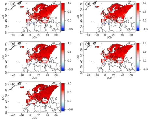
Figure 8. (a) Number of values in]0, 1]in EOBS in winter, as well as ratio (in %) of number of values in]0, 1]in winter from each BC model over that of EOBS: (b) SSR, (c) DA, (d) TA, and (e) Pos. (f ) The same ratio but between the training and projection (i.e., evaluation) periods. Upper values are censored at 400% for visualization purpose.
necessary to look at the variability of more specific types of events, such as for low precipitation values and high precipitation values. Low precipitation values are important for different aspects. For example, anoma-lously low precipitation may trigger droughts [e.g., Sivakumar et al., 2005]. Moreover, some environmental models, such as crop or vegetation models, can have different responses (e.g., in terms of growth or yields) depending on the quantity of water they receive at some time periods of the year [e.g., Lobell and Burke, 2008]. Simulating low precipitation values in a realistic manner is therefore an important need. To look at the vari-ability of the low values, the ratios (in %) of number of values in ]0, 1] in winter from each BC model over that of EOBS have been calculated per season and grid point and are displayed in Figures 8b–8e for SSR, DA, TA, and Pos, and spatially and yearly averaged ratios are given in line R]0,1]of Table 2. Except in the very north-east of the domain where DA strongly overestimates the number of low values (i.e., in ]0, 1]), the three BC models SSR, DA, and TA are similar with R]0,1]values mainly below 100%—i.e., implying an underestimation of the number of low values—for the major part of the domain, except in the northeast region with a slight overestimation. The Positive approach basically shows an underestimation in the south (R]0,1]< 100%) and a potentially strong overestimation (R]0,1]> 100%, up to more than 400%) in the north. However, all BC strate-gies present a spatial dipole (R]0,1]values lower than 100% over the south of the domain and larger than 100% over the northeast part of the domain). When comparing this spatial feature with Figure 8a—i.e., the spatial distribution of the number of values in ]0, 1]—it is visible that all the tested BC approaches underestimate this ratio R]0,1]for regions with small numbers of values in ]0, 1]. On the opposite, they tend to overestimate this ratio for regions with high numbers of values in ]0, 1]. The spatially and yearly averaged ratios (line R]0,1]in Table 2) confirm the overestimation brought by Pos (R]0,1]= 149%) and show a global underestimation for DA and TA (R]0,1]around 80%), while SSR has a R]0,1]slightly too high (108%) but the closest to 100%. This indicates that SSR produces low values with satisfactory frequencies. Note the very high value of R]0,1]for the raw WRF simulations, due to a strongly too high frequency of values in ]0, 1] in the model. Although the ranking of the BC strategies remains the same for the other seasons, R]0,1]values are in general larger for summer and slightly lower for spring and fall, emphasizing some season-specific skills of the bias correction methodologies. The variability of the high precipitation values is studied through two related criteria: the biases of the 10 year return levels from the BC data with respect to that of EOBS (hereafter referred to as B10yRL) and the percentage of BC data higher than the 95% quantile of EOBS (hereafter %> Q95). Visually, it is difficult to discriminate the four BC models based on B10yRL, as illustrated in Figures 9b–9e for winter, although the B10yRLvalues obtained from the EOBS training data show quite different values and patterns from the BC methods. Note that this is also true for the other seasons, even though the associated B10yRLvalues are larger than in winter (slightly for spring and fall and more pronounced in summer, not shown). However, when looking at averaged values of biases (line B10yRLof Table 2), the same features as previously appears, i.e., SSR, DA, and TA have smaller biases (respectively, 14.44, 18.11, and 18.06 mm) than the positive approach (24.39 mm). This also holds for the %> Q95criterion (line %> Q95of Table 2), with averaged values around 5.5% for SSR, DA, and TA and a too high value (11.23%) for Pos, which is also confirmed visually, as illustrated for winter in Figure 10 where the positive approach clearly shows %> Q95 values much larger than the optimal 5% on the major part of the domain. For those last two criteria (B10yRLand %> Q95), the raw RCM has interesting results. It has the smallest bias in 10 year return levels (B10yRL=10.2) but underestimates the number of values above the EOBS 95% quantile (%> Q95= 4%< 5%).
Interestingly, the raw RCM appears as better than some other BC methods and especially better than the Pos approach, for example, for the SB, Rvar, B10yRL, and %> Q95metrics. This could be explained by the fact that cor-recting only the positive intensities of the RCM precipitation incorporates some mismatch between the inten-sities themselves since the distribution of the positive precipitation in the RCM and that in the reference data set are not associated with similar meteorological conditions and therefore with similar rainfall properties. This strongly suggests that correcting only the positive intensities of the RCM precipitation but keeping the rainfall occurrences (and their biases) untouched tends to combine errors in occurrence modelling and errors in intensity representativity, resulting in poor results for those metrics.
As previously for the occurrence-related criteria, a rank is given among the different approaches for each of the intensity-related criteria (the lower the rank, the better), and an average rank is calculated for each approach. This time, SSR appears with rank 1.17, DA and TA both with rank 2, while the original RCM has a rank 2.67 and Pos has a rank 3.83, degrading, on average, the raw RCM. Those results tend to conclude that based on the calculated intensity-related criteria, SSR is the most reliable method among those tested to obtain bias-corrected precipitation intensities with statistical properties close to that of our reference data set.
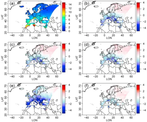
Figure 9. (a) The 10 year return levels in winter for EOBS; (b–e) biases (in mm) of the 10 year return levels from the BC
data with respect to that of EOBS, in winter, respectively, for SSR, DA, TA, and Pos. (f ) The biases of the 10 year return levels of the training period with respect to the projection (i.e., evaluation) period.
Figure 10. (a–e) Percentages of BC data higher than the 95% quantile of EOBS (projection period), respectively, for SSR,
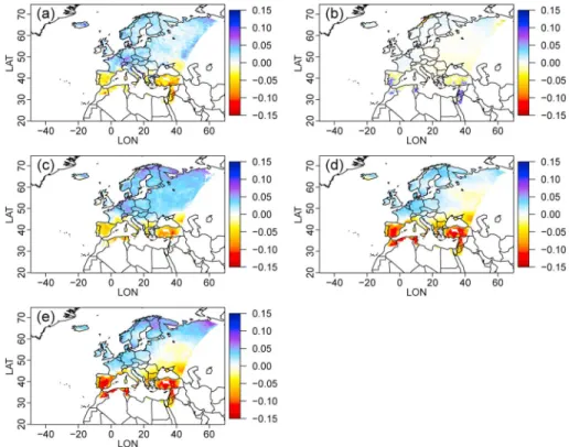
Figure 11. Mean evolution (from 1976–2005 to 2071–2100) of the wet day probabilities: (a) SSR; (b) DA; (c) TA; (d) Pos;
and (e) noncorrected RCM simulations. Values have been censored at−0.15 and +0.15 for visualization purpose.
Moreover, when calculating the same criteria over the grid points where TA cannot work, intensity-related criteria values and associated ranks given in Table 3 indicate that SSR still appears on first position with an averaged rank of 1.5, DA on second position with a rank of 2, the raw RCM on third position with rank 2.5, and Pos on last position with a rank of 3.67. As for the occurrence-related criteria, those results confirm for inten-sity the robustness of SSR to behave properly in both situations, i.e., whatever the proportion of dry days in the model with respect to that of the reference data set. Besides, in Tables 2 and 3, the respective last line dis-plays the complete averaged rank (i.e., averaged over the 10 occurrence- and intensity-related ranks) of each approach, which allows summarizing the various criteria. SSR has the best ranks (1.3 in both Tables 2 and 3), followed by DA (1.8 and 2.5), then by TA (1.8 only in Table 2, since it is not applicable in Table 3), then by the RCM (3.2 and 2.4), and finally by Pos (3.9 and 3.1).
4.3. Intercomparison of “Future” Corrected Projections
The four bias correction methods have also been applied to the 1971–2100 WRF-IPSL run, under a scenario of Representative Concentration Pathway associated with a radiative forcing of +8.5 W∕m2(RCP8.5) in the year 2100 with respect to the preindustrial period [IPCC, 2013]. In order to have a calibration data set as represen-tative as possible of the precipitation variability, the time period 1971–2005 has been used for calibration of the BC methods. The corrections have been performed on a monthly basis over the whole 1971–2100. Note that applying directly some adjustment or BC methods (like CDF-t) on different time intervals generally pro-duces discontinuities or inhomogeneities at the beginning and end of fixed time intervals. Hence, to reduce those discontinuities that are unrealistic and that could make the corrected time series nonusable in practice (for some impact models for example), in the future projection context, the models are applied based on a moving window approach, slightly adapted from Themeßl et al. [2011] as follows: For each 11 year period, the large-scale precipitation distribution is estimated based on a 21 year period (starting 5 years before the 11 year period and ending 5 years after). Hence, if information from the 21 year period is used to represent the “target” large-scale CDF, the model data are corrected only for the central 11 years. Then, the process is repeated by moving forward the temporal window by 11 years, till the end of the time period of interest. Hence, this 21/11 moving window smooths the discontinuities by incorporating temporally surrounding infor-mation and therefore consistently generates bias-corrected time series over a long period, here 1971–2100.
Figure 12. Mean evolution (from 1976–2005 to 2071–2100) of the mean daily intensities: (a) SSR; (b) DA; (c) TA; (d) Pos;
and (e) noncorrected RCM simulations. Values have been censored at−2 and +2 mm/day for visualization purposes.
Moreover, obviously, in a “future projection” context, evaluations of the corrections cannot be made against observations. Nevertheless, intercomparisons of the different approaches are performed over the 30 year 2071–2100 time period.
First, the mean yearly evolutions (i.e., averaged from the four seasonal evolution values) of the 2071–2100 wet day probability from each BC method with respect to that of the present (i.e., 1976–2005) BC data have been calculated and are shown in Figure 11. SSR, TA, and Pos have a relatively clear south-north gradient—with a diminution of the wet day probabilities in the south and an increase in the north—although some nuances are visible from one BC method to another. For example, the Pos approach shows a decrease of wet day probability around the Mediterranean basin, more pronounced than in the other methods. This was some-how expected when looking at the evolutions of these probabilities provided by the noncorrected RCM simulations (Figure 11e) that already showed the same characteristics. Interestingly, the direct approach (DA, Figure 11b) does not have such a clear gradient and even provides some increase of the wet day prob-abilities for various regions around the Mediterranean basin. Seasonal evaluations are similar to the annual ones, except for SSR that presents slightly more pronounced evolutions but with the same signs in summer (not shown).
The mean annual evolutions (mm/day) of the precipitation intensities (i.e., mean evolutions averaged from the four seasonal evolution values) has also been calculated for each BC method and are presented in Figure 12. All BC methods agree on a decrease of the intensities around the Mediterranean basin and on an increase over the northern half of the domain. This feature—in line with the evolutions seen by the uncorrected RCM simulations—is, however, more pronounced with the Positive approach (Pos, Figure 12d). Some variations can be found in the seasonal evolutions, but they all have the same signs (not shown).
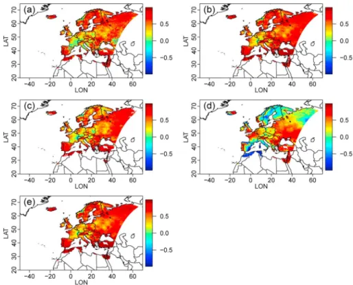
The same type of south-north gradient feature is also visible for the four methods when looking at the ratio of variance of the BC data, with the variance of the 2071–2100 BC data over that of the 1976–2005 BC data, as illustrated in Figure 13. The variability is relatively unchanged or even reduced (i.e., ratios of variance≤ 100%) around the Mediterranean, and inflated (i.e., ratios>100%) over the rest of the domain, for all BC models as
Figure 13. Mean ratios of variances (in %): var(2071–2100)/var(1976–2005) from (a) SSR; (b) DA; (c) TA; (d) Pos;
and (e) noncorrected RCM simulations. Upper values have been censored at 400% for visualization purpose.
well as for the uncorrected RCM values. From a seasonal point of view, the winter, spring, and fall evolutions of variance are similar to each other. However, more variability is present in summer for all BC, especially for TA (not shown), implying a much larger precipitation variability in 2071–2100 summers than in historical ones.
5. Conclusions and Discussions
This study focused on how the treatment of the rainfall occurrences in a bias correction methodology con-text may affect the adjusted precipitation, both in terms of occurrence properties and in terms of intensity. Three different methodologies have been compared—namely, the “direct approach” (DA), the “Threshold Adaptation” approach (TA), and the “Positive Approach” (Pos)—as well as a method called “Singularity Stochastic Removal” (SSR), all based on the CDF-t adjustment model . The direct approach consists in applying an adjustment model directly on the whole time series including both dry days and rainy days, i.e., without separating the correction methodology into occurrence and intensity. The Threshold adaptation approach consists in finding a threshold t such that the proportion of days with model precipitation< t is the same as the proportion of dry days in the reference (observed) precipitation data set, putting those model precipita-tion values to zero and adjusting only the positive model values (i.e.,> t). However, TA is only applicable when the model precipitation to be corrected has too many wet days (i.e., not enough dry days). As for the positive approach, it only corrects the positive intensities of precipitation, without correcting the dry events.The SSR method allows removing subcases in dealing in the same way with the situations where the model to be cor-rected has too many wet days or not. For that, SSR replaces all model and reference precipitation lower than a value th (selected small enough by the user) by a random value uniformly distributed between 0 and th, performs an adjustment onto the whole newly obtained time series, and puts to zero the bias-corrected data lower than th. Hence, SSR also avoids separating the correction of the occurrence from that of the intensity, which constitutes a flexible tool.
Those four approaches have been first applied in a cross-validation framework to bias correct a precipitation run from the WRF regional climate model forced by the IPSL GCM. When TA was applicable (Table 2), in terms of occurrence properties, SSR, DA, and TA were relatively satisfactory and close to each other, while the results
of the Pos approach were usually much more biased. However, in terms of intensity, if Pos still appeared much more biased than the other three BC methods, SSR had a slight advantage over DA and TA. In general, SSR provided the best results when all (i.e., occurrence- and intensity-related) criteria were accounted for. This was even more true in the case when TA was not applicable (Table 3), i.e., when the model precipitation to be corrected had too many dry days. In this case, SSR clearly provided the best results for most of the criteria (both in terms of occurrences and intensities). Interestingly, if DA appeared second best in general and for intensity-related criteria, this does not hold for all occurrence properties, where the positive approach (i.e., with the occurrences of the model to be corrected) may be better than DA. In other words, correcting the model with the direct approach can sometimes degrade the occurrence properties.
For most of the occurrences-related criteria, the spatial patterns present in the EOBS training data set (compared to that of the evaluation period) are generally reproduced by the different BC models, in the sense that the spatial structure of their biases somehow looks like the spatial structure of the evolutions of the statis-tical properties of precipitation from the training to the projection periods. This is an indication that although SSR, DA, and TA have been designed to be applicable in climate conditions different from the climate of the calibration period, they have a general tendency to stay close to the occurrence characteristics of the training data set. This is nevertheless not completely the case when looking at intensity-related criteria for which the variance ratio criterion and the biases of the 10 year return levels are quite different for the BC models and the EOBS training data set. Interestingly, for some intensity-related criteria, the raw WRF simulations provide better results than the positive approach that can degrade the raw RCM simulations.
The four bias correction techniques have also been applied to correct future precipitation over the 2071–2100 period. Even though evaluations are not possible, a brief intercomparison has been realized. The different BC methods showed relatively equivalent evolutions from 1976–2005 to 2071–2100 in terms of wet day prob-abilities, mean daily intensities, and variances: The edge of the Mediterranean sees a decrease of probability and intensity of precipitation associated with a reduction of the variability, while the rest of Europe displays an increase of precipitation with a larger variability. This result is in line with previous studies [e.g., Christensen
and Christensen, 2007; IPCC, 2013] showing an increase of precipitation in the north of Europe. However, some
differences existed, such as the following: only small wet day probabilities evolutions were provided by DA compared to the others; more pronounced (positive and negative) mean intensity evolutions for the Pos approach; and larger evolution of the summer variability for TA.
Although some differences may appear depending on the criteria, corrections of other RCM-GCM runs give equivalent results and rankings (not shown), implying some robustness in the conclusions brought by this study.
As a global conclusion, the “Singularity Stochastic Removal” BC method is a good compromise to correct both precipitation occurrences and intensities, whether the model has too many dry or too many wet days. The perspectives of this work are numerous. A first one is to extend the number of criteria utilized here to evaluate the various BC strategies. For example, a focus could be made on climate extremes, based on some indices defined by the so-called “Expert Team on Climate Change Detection and Indices” (ETCCDI) [see Zhang
et al., 2011]. The results could be threshold dependent, and the 0 mm wet day threshold used in the present
study may have therefore to be changed to show differences.
Another perspective is to apply SSR to more RCM-GCM runs. Such an ensemble of bias-corrected RCM-GCM runs would improve the quality of the uncertainty assessment in the historical framework and help to understand the variability of the projections in a climate change context. A work in that direction has already started through the correction of the EURO-CORDEX runs. The SSR method has been applied for bias correc-tion of EURO-CORDEX precipitacorrec-tion for the French nacorrec-tional report on climate scenarios [Ouzeau et al., 2014], using a high-resolution data set for France. It has also been applied to EURO-CORDEX projections at the scale of Europe the “Climate Information Platform for Copernicus” (CLIPC) project (see downloadable files on http://exporter.nsc.liu.se/e4ba1c00373c4b548b12c30b269a1c98/).
Besides, it would be interesting to extend SSR in a multivariate context. So far, it has only been applied in a univariate framework (i.e., one location and one variable at a time). Allowing SSR to work in accounting for intervariable dependences or spatial properties could bring valuable additional information to improve the final corrections. To do so, adapting SSR to the approach developed by Piani and Haerter [2012] for


![Figure 8. (a) Number of values in ]0 , 1] in EOBS in winter, as well as ratio (in %) of number of values in ]0 , 1] in winter from each BC model over that of EOBS: (b) SSR, (c) DA, (d) TA, and (e) Pos](https://thumb-eu.123doks.com/thumbv2/123doknet/13343715.401816/14.918.303.820.639.1055/figure-number-values-eobs-winter-number-values-winter.webp)