HAL Id: hal-01373715
https://hal.inria.fr/hal-01373715
Submitted on 30 Sep 2016
HAL is a multi-disciplinary open access
archive for the deposit and dissemination of
sci-entific research documents, whether they are
pub-lished or not. The documents may come from
teaching and research institutions in France or
abroad, or from public or private research centers.
L’archive ouverte pluridisciplinaire HAL, est
destinée au dépôt et à la diffusion de documents
scientifiques de niveau recherche, publiés ou non,
émanant des établissements d’enseignement et de
recherche français ou étrangers, des laboratoires
publics ou privés.
Highly Reduced Model of the Cardiac Function for Fast
Simulation
Marc-Michel Rohé, Roch Molléro, Maxime Sermesant, Xavier Pennec
To cite this version:
Marc-Michel Rohé, Roch Molléro, Maxime Sermesant, Xavier Pennec. Highly Reduced Model of the
Cardiac Function for Fast Simulation. IEEE - IVMSP Workshop 2016, Jul 2016, Bordeaux, France.
pp.5, �10.1109/IVMSPW.2016.7528214�. �hal-01373715�
HIGHLY REDUCED MODEL OF THE CARDIAC FUNCTION FOR FAST SIMULATION
Marc-Michel Roh´e, Roch Moll´ero, Maxime Sermesant and Xavier Pennec
Inria Sophia-Antipolis, Asclepios Research Group, Sophia-Antipolis, France
ABSTRACT
In this article we present a drastic dimension reduction method to link the biophysical parameters of an electrome-chanical model of the heart with a compact representation of cardiac motion. Our approach relies on a projection of the displacement fields along the whole cardiac motion to the space of reduced-polyaffine transformations. Using these transformations, not only we describe the motion using a very small number of parameters but we show that each of these parameters has a physiological meaning. Moreover, using a PLS regression on a learning set made of a large number of simulations, we are able to find which of the input parameters of the model most impact the motion and what are the main relations mapping the polyaffine representation to the param-eters of the model. We illustrate the potential of this method for building a direct and very fast model characterized by a highly reduced number of parameters.
1. INTRODUCTION
Modelling of the heart had an increasing interest in the recent years as it provides a way to better assess the cardiac function and predict its evolution. In order to estimate subject-specific model parameters, cardiac motion is often used, as it can be extracted from medical images. However, given the complex dynamics of cardiac motion, its analysis and its link with the underlying physical parameters of the cardiac tissue are diffi-cult to achieve. This complexity of the model is due to differ-ent factors: the number of input parameters, the complexity of the cardiac motion - represented by 3D-vector fields defined for a temporal discretization of the cycle - and the non-linear relationship between the input and output. In this article, we introduce a new method to reduce a cardiac motion model to very few parameters by reducing the dimension of the output motion and estimating the main modes of variation linking biophysical parameters and cardiac motion.
A cardiac biophysical model can be described as a func-tion f which maps a geometry S (discretely represented by a
segmented mesh: a finite set of points in R3) and a set of input
parameters Θ = (θi)i=1,...,Qto the simulation of the motion
of this geometry through the cardiac cycle M = (St)0<t<1:
M = (St)0<t<1= f (S0, θ1, ..., θi, ..., θM). (1)
In order to reduce such model, we first need to be able
to express the cardiac motion M = (St)0<t<1by a reduced
number of parameters M = (mj)j=1,...,N. To do so, we use
a polyaffine projection [1] which we further develop by ex-pressing the parameters on a basis adapted to the heart geom-etry and his motion [2]. In this new frame we only project on the 6 (instead of 12 for standard affine) most relevant param-eters. We show that, not only the parameters of this reduced-polyaffine projection gives a very good approximation of the whole cardiac motion, but also that each of these parameters is physiologically interpretable. We then learn the relation between both the reduced-polyaffine parameters M and the input parameters Θ of the model with a Partial Least Square (PLS) regression. We build a direct forward model using only a highly reduced number of parameters and show for 100 test simulations that we are able to reconstruct the motion directly using our surrogate model given by the the first modes of the PLS regression that is very close to the full model computa-tion while being way faster to compute.
Such approach is a hybrid method between recently de-veloped hyper-reduced models, looking for a lower dimen-sional representation of the spatial state variables [3] and the meta-models, looking for correlations between input and out-put of models [4]. One important difference is that we explic-itly define the first dimension reduction in the spatial domain in order to have meaningful parameters, related to regional deformations. These parameters define transformations that are independent of the spatial frame and position chosen and therefore can be extended as such for any new geometry.
2. REDUCED-POLYAFFINE PROJECTION FOR COMPACT CARDIAC MOTION REPRESENTATION In this section, we propose a method to project a given cardiac motion M to a subspace of finite dimension in which it will
be represented by a set of parameters M = (mj)j=1,...,N:
π : M → M = (m1, ..., mj, ..., mN).
We suppose we have a cardiac motion represented on a temporal discretization of the cycle by T displacements fields ( ˜Dt)t=1,...,T mapping each point of the initial mesh S0to the
corresponding point of the mesh St at frame t. Instead of
looking at displacements fields, we choose to represent the cardiac motion by stationary velocity fields (SVF) such that
0 5 10 15 20 25 30 0 1 2 3 4 5 6 7 Frames Ditance (mm) Absolute displacement Error of the polyaffine projection
0 5 10 15 20 25 30 35 −0.1 0 0.1 0.2 0.3 0.4 0.5 0.6 0 5 10 15 20 25 30 35 −0.2 −0.15 −0.1 −0.05 0 0.05 0 5 10 15 20 25 30 35 −0.5 −0.4 −0.3 −0.2 −0.1 0 0.1 0.2
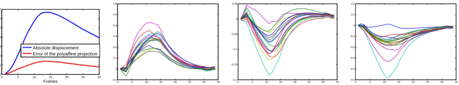
Table 1. Polyaffine projection for a cardiac motion. (Left) figure: error of the projection versus absolute displacement. (Right) figures: diagonal parameters over time of the polyaffine matrix for each of the region of the left ventricle from which we can recognize (resp. from left to right) the radial, longitudinal and circumferential strains.
˜
vt = log ˜Dt. As described in [5], working with SVF allows
us to perform vectorial statistics on diffeomorphisms, while preserving the invertibility constraint, contrary to the Euclid-ian statistics on displacement fields. Since the space of the SVF is dense, we need to reduce the dimension by projection onto a lower dimensional space. To do so, we will use the polyaffine projection [1].
By defining K regions and associated smooth weights, we describe locally affine deformations using few parameters while still being globally invertible. The polyaffine transfor-mation is the weighted sum of these locally affine transforma-tions: vpoly(x) = K X k=1 ωi(x)Mix.˜
We use the standard American Heart Association (AHA) 17 regions for the left ventricle. We also define 10 additional re-gions dividing the right ventricle in a similar way for a total
of K = 27 regions. The weights ωi are normalized
Gaus-sian function around the barycentre of each region [1]. The parameters of the optimal projection of a Stationary Velocity Fields v onto the space of polyaffine transformations has an
analytical solution m = ˆm = Σ−1b [6] which minimizes in
the least-square sense:
C(m1, ..., mN) = Z Ω kX i vpoly(x) − v(x)k2dx.
In order to get interpretable parameters for each region, we chose to express them in a local coordinate system adapted to the geometry of the heart.
Calling R = (O, e1, e2, e3)
the original Cartesian coordinate system, we define the local
coor-dinate of the region k as R0i =
(Ok, e1k, e2k, e3k) where Ok is
the barycenter of the region (the red point in the enclosed figure),
e1 the radial vector (green
vec-tor), e2 the longitudinal vector
(purple vector) and e3 the
cir-cumferential vector (blue vector).
We can express the 12 affine parameters of the 3 × 4
ma-trix Miin this new frame. Doing so makes these parameters
independent of the global frame R on which we are looking the motion. Therefore, these parameters are comparable be-tween different geometries so that the study can be extended to multiple patients. Furthermore, we propose a method to re-duce further the representation of the motion by keeping only the most important parameters out of the 12 parameters of the affine matrix. As stated in [2], when expressed in the local basis, the diagonal parameters of the rotation part R of the affine matrix (representing the strain in the 3 directions: ra-dial, longitudinal and circumferential) as well as the 3 trans-lation parameters representing the displacements are the most prominent in explaining the motion. Keeping only these 6 pa-rameters leads to a reduction of half of the complexity of our representation of the motion while keeping clinically signifi-cant parameters.
We show the results of the polyaffine projection - keep-ing 6 parameters per regions - for a whole cardiac motion in Fig. 1. The projection has a mean absolute error below 1mm,
and we explain more than 80% of the original motion (in L2
norm of the velocity field with respect to the whole displace-ment). Keeping all the 12 parameters would only slightly im-prove the projection (mean bsolute error approx. 10% lower) while increasing the complexity. Finally we see that the 3 di-agonal parameters gives a good account of the 3 strains and the curves are in accordance with clinical knowledge: posi-tive radial strains (approx. 30 % at end-systole) and negaposi-tive longitudinal and circumferential strains (approx. −10% and −15% at end-systole).
3. BIOPHYSICAL MODEL OF THE HEART SIMULATION DATABASE
We use a cardiac mechanical model based on the Bestel-Clement-Sorine (BCS) modeling [7]. This model describes the heart as a Mooney Rivlin passive material, and model the stress along the cardiac fibres according to microscopic scale phenomena. Particularly, this model is compatible with the laws of thermodynamics. It also integrates a circulation model representing the 4 phases of the cardiac model, where
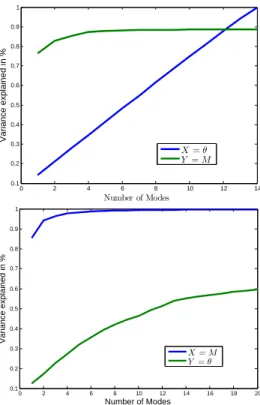
0 2 4 6 8 10 12 14 0.1 0.2 0.3 0.4 0.5 0.6 0.7 0.8 0.9 1 Number of Modes Variance explained in % X = θ Y = M 0 2 4 6 8 10 12 14 16 18 20 0.1 0.2 0.3 0.4 0.5 0.6 0.7 0.8 0.9 1 Number of Modes Variance explained in % X = M Y = θ
Table 2. (Top) row: PLS regression with X = θ the predictor variable and Y = M the dependant variable. (Bottom) row: X = M and Y = θ. (Left) figure: variance explained by the PLS regression with respect to the number of modes. (Right) figure: VIP of each of the parameters.
the aortic pressure is modelled by a 4-parameter Windkessel model. Finally, the electrophysiological pattern of activity is simulated using an Eikonal model, describing the depo-larization front propagation from the endocardial surface
to the whole myocardium. Fourteen parameters are used
by the model: (σ0, krs, katp, k0, α, µ, Es) active
parame-ters, (K, c1, c2) passive parameters and (Rp, τ, Zc, L) for the
valve model. We simulate S = 500 cardiac cycles whose input parameters are drawn randomly according to a uniform distribution within a range of parameters chosen as to obtain a physiologically realistic behaviour (following the sensitivity analysis of the model done in [8]). In total, each simulation
has therefore Q = 14 specific parameters Θ = θi=1,...,Qof
the model. On the other side, for each of these motions we calculate the N = 6 × K × T reduced-polyaffine parameters
M = (ml,k,t)l=1,...6,k=1,...K,t=1,..,T = (mj)j=1,...,N.
4. PARAMETERS MAPPING THROUGH PLS REGRESSION
In this section, we are looking to link the polyaffine param-eters M with the input paramparam-eters of the cardiac model Θ. PLS regression finds the multidimensional direction in the X (the predictors variables) space that explains the maximum multidimensional variance direction in the Y space (the de-pendant variables) [9]. It combines both features from the
PCA (the projection of Y and X into subspaces of high vari-ance) and standard linear regression (by the search of linear relations between the modes of X and Y ). With X the pa-rameters of the polyaffine and Y the papa-rameters of the model, PLS returns the modes in the space of the polyaffines trans-formation which have maximum variance and maximum co-variance with the parameters of the model Y . It is more ro-bust than standard regression when the space of X and Y is highly-dimensional because of the embedded dimension re-duction when looking for linear relations.
With our two sets of parameters Θ = θi and M = mj,
we can either try to predict the parameters M from the param-eters Θ and use this relation to build a highly reduced direct model as we show in section 5, or we can estimate the relation between the parameters Θ of the model from the polyaffine parameters M of the motion to study the part of the motion impacted the most by changes in the parameters of the model. We therefore compute the PLS regression both with X = Θ the predictor variable and Y = M the dependant variable and with X = M and Y = Θ.
In Fig. 2, we show the variance explained by the PLS re-gression with respect to the number of modes used. With only 5 modes, we can explain more than 90% of the polyaffine pa-rameters variance using only 30% of the variance of the car-diac model parameters. This shows that most of the impact of the parameters of the model can be explained by only few
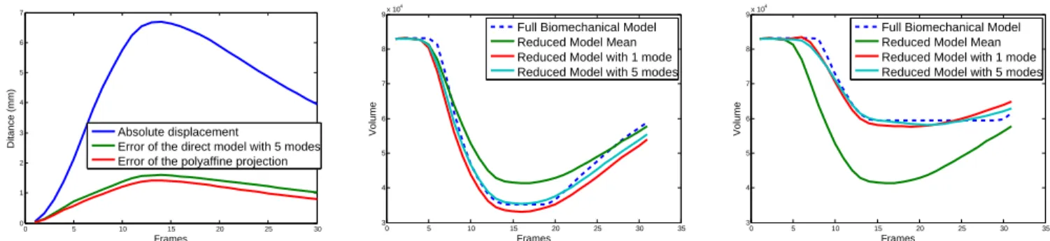
0 5 10 15 20 25 30 0 1 2 3 4 5 6 7 Frames Ditance (mm) Absolute displacement
Error of the direct model with 5 modes Error of the polyaffine projection
0 5 10 15 20 25 30 35 3 4 5 6 7 8 9x 10 4 Frames Volume
Full Biomechanical Model Reduced Model Mean Reduced Model with 1 mode Reduced Model with 5 modes
0 5 10 15 20 25 30 35 3 4 5 6 7 8 9x 10 4 Frames Volume
Full Biomechanical Model Reduced Model Mean Reduced Model with 1 mode Reduced Model with 5 modes
Table 3. (Left) figure: mean absolute displacement of the motion and mean absolute error of the direct model. (Right) and
(Middle) figures: Left ventricular volume curve (mm3) defined by the direct model versus the full model for two extreme
simulated cases: one with high ejection fraction and one with low ejection fraction.
of the input variable and that 70% of the variance of the pa-rameters of the model impacts the motion represented by the polyaffine parameters by only 10%. On the other side, we do not predict as well the parameters Y = Θ, which could be ex-plained by issues of identifiability in the model (several sets of input parameters leading to very close motions), a known fact in complex cardiac motion models. But the parameters we predict are highly correlated to actual change in the mo-tion looking at the explained variance of X = M with only few modes.
We also calculate the Variable Importance in the Projec-tion (VIP) [10] for both of our regression with 5 modes. VIP compares the variance explained by the modes of the PLS re-gression for each of the variable in X. Variables with high impact on the dependant variables will be well estimated by the modes of X and have high VIP factor. The parameters shown in red are the one that were considered as the most im-portant for personalization in [8]. Our statistical analysis con-firms these findings by quantifying the importance of each of these parameters with the VIP. Finally, the analysis of the VIP for the other way shows that radial strain and contraction are the most important motion features to explain the parameters of the model, which is physiologically expected.
5. DIRECT HIGHLY REDUCED CARDIAC FUNCTION MODEL
In this section, we build a surrogate cardiac model using the PLS modes of X and Y and the linear relation found previously. Our reduced model can be expressed as a linear function g approximating the function f from equation 1 and expressed with only L parameters, the PLS modes, which linearly map the Q inputs of the model Θ to the N polyaffine parameters M. This surrogate model has two sources of error compared to the full model. First, the subspace of polyaffine transformations already gives an approximation of the full motion as seen in Section 2, so that the projection of the motion on this subspace is an approximation. Secondly, the polyaffine parameters are estimated from the PLS modes and
are only approximating the optimal polyaffine parameters given by the projection.
We perform 100 new test simulations and show in Fig. 3 how well our highly reduced model approximates the motion given by the full model. The mean error of the points of the mesh along motion stays below 2mm meaning that we ex-plain more than 75% of the complete motion. The impact on the volume curve of using an increasing number of modes on top of just the mean parameters is shown for two sim-ulations: one with high ejection fraction and one with low ejection fraction. The first mode already approximates quite well the volume curve for these two extreme cases, showing that this mode is highly correlated with change in the ejection fraction. We can infer that the most prominent variation of the model is related to the ejection fraction (the ratio between the min. volume and the max. volume) which is physiologically expected as it is the most important characteristic to asses the cardiac function efficiency. Adding additional modes to the PLS regression improves the approximation of the reduced model.
6. CONCLUSION
In this paper, we proposed an innovative methodology to re-duce a whole biophysical cardiac model using polyaffine pro-jection and PLS regression. While the initial model is very complex (as a non-linear application from a large number of parameters to the whole space of displacement fields) and takes about 2 − 3 hours to run on a quad-core 2.10GHz CPU, we are able to explain it with good accuracy with only a cou-ple of modes of a surrogate simplified model running in less than 2 minutes, which still gives an accurate estimation of the ejection fraction. Extension of this method to other inputs of a cardiac function model such as electrophysiology might be possible and give further insight into how each input compo-nent impacts the model. The inverse relation found by the PLS regression (between the motion and the model param-eters) could also be used to tackle the inverse problem and efficiently personalize the model.
The authors acknowledge the partial funding by the EU FP7-funded project MD-Paedigree (Grant Agreement 600932)
7. REFERENCES
[1] Kristin Mcleod, Christof Seiler, Nicolas Toussaint, Maxime Sermesant, and Xavier Pennec, “Regional anal-ysis of left ventricle function using a cardiac-specific polyaffine motion model,” in Functional Imaging and Modeling of the Heart. 2013, pp. 483–490, Springer. [2] Marc-Michel Roh´e, Nicolas Duchateau, Maxime
Ser-mesant, and Xavier Pennec, “Combination of Polyaffine Transformations and Supervised Learning for the Auto-matic Diagnosis of LV Infarct,” in Statistical Atlases and Computational Modeling of the Heart (STACOM 2015), Munich, Germany, 2015.
[3] D. Ryckelynck, “Hyper-reduction of mechanical models involving internal variables,” International Journal for Numerical Methods in Engineering, vol. 77, no. 1, pp. 75–89, 2009.
[4] Kristin Tøndel, Ulf G Indahl, Arne B Gjuvsland, Stig W
Omholt, and Harald Martens, “Multi-way
metamod-elling facilitates insight into the complex input-output maps of nonlinear dynamic models,” BMC Systems Bi-ology, vol. 6, no. 1, pp. 88, 2012.
[5] Vincent Arsigny, Olivier Commowick, Xavier Pennec, and Nicholas Ayache, “A log-Euclidean framework for statistics on diffeomorphisms,” in Proc. of the 9th Inter-national Conference on Medical Image Computing and Computer Assisted Intervention (MICCAI’06), Part I, 2-4 October 2006, number 2-4190 in LNCS, pp. 922-4–931. [6] Christof Seiler, Xavier Pennec, and Mauricio Reyes,
“Capturing the multiscale anatomical shape variability with polyaffine transformation trees,” Medical Image Analysis (MedIA), vol. 16, no. 7, pp. 1371–1384, 2012. [7] Julie Bestel, Fr´ed´erique Cl´ement, and Michel Sorine,
“A biomechanical model of muscle contraction,” in
Medical Image Computing and Computer-Assisted Intervention–MICCAI 2001. Springer, 2001, pp. 1159– 1161.
[8] St´ephanie Marchesseau, Herv´e Delingette, Maxime Ser-mesant, and Nicholas Ayache, “Fast parameter calibra-tion of a cardiac electromechanical model from medical images based on the unscented transform,” Biomechan-ics and Modeling in Mechanobiology, 2012.
[9] Roman Rosipal and Nicole Kr¨amer, “Overview and re-cent advances in partial least squares,” in Subspace, la-tent structure and feature selection, pp. 34–51. Springer, 2006.
[10] Thanh N. Tran, Nelson Lee Afanador, Lutgarde M.C. Buydens, and Lionel Blanchet, “Interpretation of vari-able importance in partial least squares with significance multivariate correlation (smc),” Chemometrics and In-telligent Laboratory Systems, vol. 138, pp. 153–160, 2014.