HAL Id: hal-01644285
https://hal.inria.fr/hal-01644285
Submitted on 22 Nov 2017
HAL is a multi-disciplinary open access
archive for the deposit and dissemination of
sci-entific research documents, whether they are
pub-lished or not. The documents may come from
teaching and research institutions in France or
abroad, or from public or private research centers.
L’archive ouverte pluridisciplinaire HAL, est
destinée au dépôt et à la diffusion de documents
scientifiques de niveau recherche, publiés ou non,
émanant des établissements d’enseignement et de
recherche français ou étrangers, des laboratoires
publics ou privés.
Uncertainty-Aware Hybrid AADL Designs Using
Statistical Model Checking
Yongxiang Bao, Mingsong Chen, Qi Zhu, Tongquan Wei, Tingliang Zhou,
Frédéric Mallet
To cite this version:
Yongxiang Bao, Mingsong Chen, Qi Zhu, Tongquan Wei, Tingliang Zhou, et al.. Quantitative
Per-formance Evaluation of Uncertainty-Aware Hybrid AADL Designs Using Statistical Model Checking.
IEEE Transactions on Computer-Aided Design of Integrated Circuits and Systems, IEEE, 2017, 36
(12), pp.1989 - 2002. �10.1109/TCAD.2017.2681076�. �hal-01644285�
Quantitative Performance Evaluation of Uncertainty-Aware
Hybrid AADL Designs Using Statistical Model Checking
Yongxiang Bao, Mingsong Chen
∗Member, IEEE, Qi Zhu Member, IEEE, Tongquan Wei Member, IEEE,
Frederic Mallet Member, IEEE and Tingliang Zhou
Abstract— Architecture Analysis and Design Language (AADL) is widely used for the architecture design and analysis of safety-critical real-time systems. Based on the Hybrid annex which supports continuous behavior modeling, Hybrid AADL enables seamless interactions between embedded control systems and continuous physical environments. Although Hybrid AADL is promising in dependability prediction through analyzable architecture development, the worst-case performance analysis of Hybrid AADL designs can easily lead to an overly pessimistic estimation. So far, Hybrid AADL cannot be used to accurately quantify and reason the overall performance of complex systems which interact with external uncertain environments intensively. To address this problem, this paper proposes a statistical model checking based framework that can perform quantitative evalua-tion of uncertainty-aware Hybrid AADL designs against various performance queries. Our approach extends Hybrid AADL to support the modeling of environment uncertainties. Furthermore, we propose a set of transformation rules that can automatically translate AADL designs together with designers’ requirements into Networks of Priced Timed Automata (NPTA) and perfor-mance queries, respectively. Comprehensive experimental results on the Movement Authority (MA) scenario of Chinese Train Control System Level 3 (CTCS-3) demonstrate the effectiveness of our approach.
Index Terms— Hybrid AADL, Uncertainty, Statistical model checking, Quantitative performance evaluation.
I. INTRODUCTION
T
O promptly and accurately sense and control the physical world, more and more real-time embedded systems are deployed into our surrounding environment. As a result, the stringent safety-critical requirements coupled with increasing interactions with uncertain physical environments make the design complexity of Cyber-Physical Systems (CPS) skyrock-eting [1], [2]. Unfortunately, due to the lack of architecture-level performance evaluation approaches considering uncertain environments, the required performance of integrated CPS implementations can be easily violated. Therefore, how to model the uncertain behaviors of both cyber and physical elements and how to guarantee meeting the critical functional and real-time requirements have become major challenges in CPS architecture design.The authors Yongxiang Bao, Mingsong Chen, and Tongquan Wei are with Computer Science and Software Engineering Institute at East China Normal University, Shanghai, 200062, China. The author Qi Zhu is with Department of Electrical and Computer Engineering at University of California, Riverside, CA 92521, USA. The author Frederic Mallet is with University Nice Sophia Antipolis, F-06902 Sophia Antipolis Cedex, France. Tingliang Zhou is with Casco Signal Ltd., Shanghai, 200070, China.
∗Corresponding author. Tel: +(8621) 62235116; fax: +(8621) 62235255.
E-mail address: [email protected]
As a component-oriented modeling language, Architecture Analysis and Design Language (AADL) [3], [4] has been widely adopted in the design and analysis of safety-critical real-time systems (e.g., automotive, avionics and railway sys-tems). By defining various modeling constructs for hardware and software components, AADL core language supports the structural description of system partitioning and connectivity between components, while the semantics of AADL can be ex-tended via annex sublanguages and user-defined properties. To increase comprehension about a system and enhance the prob-ability of successful implementations, an AADL specification provides a set of modeling constructs for the description and verification of both functional and non-functional properties of interactive software and hardware components. Since the core AADL language only supports modeling of hardware and software components, to model the physical environment we adopt the Hybrid AADL, which supports continuous behavior modeling via Hybrid annex [5].
When modeling a safety-critical system using AADL, be-fore the design refinement, there is a rigorous certification process to verify whether the properties of the AADL design are satisfied. Although existing AADL IDE tools such as OSATE [6] can be used to check timing properties (e.g., flow latency), most of existing approaches adopt the worst-case timing analysis without considering performance variations, which can easily lead to an overly pessimistic performance estimation. To extend the performance analysis capability of AADL designs, various model transformation approaches [7], [8] have been proposed to verify AADL models based on exist-ing verification and analysis tools. For the quantitative analysis of uncertainty-aware AADL designs, designers would like to ask the question “What is the probability that a specified scenario can be achieved within time x?”. However, existing approaches focus on the safety property checking which only have an answer of “yes” or “no” without considering uncertain environments. Few of them can quantitatively reason why a given performance requirement cannot be achieved and answer how to improve the design performance. Clearly, the bottleneck is the lack of powerful quantitative evaluation approaches that can help AADL designers to make decisions during the architecture design.
To enable the quantitative analysis for Hybrid AADL de-signs, we propose a novel framework based on Statistical Model Checking (SMC) [9], [11] which relies on the mon-itoring of random simulation runs of systems. By analyzing the simulation results using the statistical approaches (e.g., sequential hypothesis testing or Monte Carlo simulation), the satisfaction probability of specified properties (i.e.,
formance requirements) can be estimated. Unlike traditional formal verification methods which need to explore all the state space, SMC only investigates a limited number of simulation runs of systems, which requires far less memory and time. Therefore, SMC is very suitable for the approximate functional validation of complex AADL designs. We use the statistical model checker UPPAAL-SMC [10], [11] as the engine of our approach, to leverage its rich modeling constructs and flexible mapping mechanisms. Based on UPPAAL-SMC, this paper makes three following major contributions: i) We extend the syntax and semantics of Hybird AADL specifications [5] using our proposed Uncertainty annex, which enables the accurate modeling of both performance variations caused by uncertain environments and performance requirements spec-ified by designers. ii) To automate the quantitative analysis of uncertainty-aware Hybrid AADL designs, we adopt the Network of Priced Timed Automata (NPTA) [9] as the model of computation in our approach. We propose a set of map-ping rules that can automatically transform uncertain-aware Hybrid AADL designs into NPTA models and convert the performance requirements into various kinds of queries in the form of cost-constrained temporal logic [12]. iii) Based on our proposed SMC-based evaluation framework, we implement a tool chain which integrates both UPPAAL-SMC and the open-source AADL tool environment OSATE to enable the auto-mated performance evaluation and comparison of uncertainty-aware Hybrid AADL designs.
The rest of this paper is organized as follows. After intro-ducing the related work on AADL and SMC-based evaluation in Section II, Section III presents the details of our approach. Based on an industrial CTCS-3 MA design, Section IV shows that our proposed approach can be effectively applied to the quantitative analysis of Uncertain Hybrid AADL designs. Finally, Section V concludes the paper.
II. RELATEDWORK
To facilitate architecture design and analysis of safety-critical systems, various AADL simulation and verification tools were investigated based on extended annexes. For exam-ple, Jahier et al. [13] proposed an approach that can translate both AADL models and software components developed in synchronous languages (i.e., SCADE, Lustre) into executable models, which can be simulated and validated together. In [14], Al-Nayeem et al. developed a modeling framework in AADL to automatically transform the synchronous design of a real-time distributed system into an asynchronous design satisfying the Physically-Asynchronous Logically-Synchronous (PALS) protocol. Furthermore, they developed a static analysis checker to find necessary conditions that must be satisfied for the cor-rect PALS transformation. In [16], Larson et el. introduced the Behavioral Language for Embedded Systems with Software (BLESS) annex for AADL. The extended AADL language together with the developed BLESS proof tool enable the implementation verification against the specified specification. In [18], Bodeveix et al. proposed a verification toolchain for AADL models through their transformation to the Fiacre language. They investigated the semantics of AADL models
and Fiacre subsets expressed in a common framework. Al-though these approaches are promising in functional checking of AADL designs, few of them consider performance issues for safety-critical systems.
Rather than developing dedicated verification tools for AADL designs, more and more model transformation-based AADL analysis approaches resort to the benefits of widely-used model checking [19] and theorem proving techniques [5], [25]. For instance, Bj¨ornander et al. [15] extended the semantics of AADL using a behavior annex with time annota-tions. By mapping AADL designs to the Timed Abstract State Machines (TASM) language, their approach allows timing analysis with timed simulation or timed model checking. Similarly, Hu et al. [7] presented a set of formally defined rules that can translate a subset of AADL to corresponding Timed Abstract State Machines (TASM) models for the purpose of timing and resource verification. To ensure completeness and consistency of an AADL specification as well as its conformity with the end product, Johnsen et al. [8] presented a formal verification technique by translating AADL designs to timed automata models. In [26], Wei et al. developed a safety verification approach called QaSten for AADL designs by transforming them into probabilistic models, which can be checked by the model checker PRISM. Due to the increasing interactions with physical environments, the support of hybrid behavior modeling and verification is becoming an important research topic in AADL design. For example, based on BLESS annex [16] and Hybrid annex [5], Ahmad et al. [21] investi-gated the modeling and analysis of the movement authority scenario of the Chinese Train Control System Level 3 (CTCS-3) in AADL. Their approach can verify both discrete and hybrid behaviors of annotated Hybrid AADL designs based on the interactive Hybrid Hoare Logic prover [17]. Although there exist dozens of methods that can be used to verify the correctness and dependability of safety-critical AADL designs, very few of them take the uncertain physical environment into account. Unlike tranditional theorem provers which focus on proving functional correctness rather than reasoning design performance, the simulation-based UPPAAL-SMC used in our approach can be fully automated without manual “proof as-sistants”. Moreover, UPPAAL-SMC requires far less memory and time, which allows high scalable validation.
Due to the scalability and effectiveness in evaluating stochastic behaviors of systems, statistical model checking [22] is becoming a preferred option in the uncertainty-aware performance analysis of system designs. Based on UPPAAL-SMC, Chen et al. [23] proposed an approach that can model the process of MPSoC task allocation and scheduling under time and power variations. By using their method, inferior resource allocation and scheduling solutions can be filtered, thus the performance yield of MPSoC chips can be improved. In [24], Bruintjes et al. introduced a statistical approach for timed reachability analysis of extended AADL designs. They developed a simulator that can perform probabilistic analysis of underlying stochastic models using Monte Carlo simulation. Our approach differs greatly from [24]. In [24], the extended AADL is based on linear-hybrid models, whereas our approach supports the modeling of nonlinear behaviors for a large group
of CPSs. In particular, the clock rates in UPPAAL-SMC can be described using ordinary differential equations [11], e.g., c10== sin(c2), c10== c1 ∗ c2 + c3, where c1, c2 and c3 are three clock variables. In addition to the capability of model-ing nonlinear behaviors, our approach focuses on evaluatmodel-ing CPS performance under uncertain environments, while [24] puts emphasis on the error behavior modeling of hardware and software components. Moreover, [24] only considers the probability of event occurrences and delay variations following either uniform or exponential distributions, while our approach allows designers to define their own uncertain objects (e.g., system parameters, user inputs) following a wide spectrum of programmable distributions. Furthermore, the method in [24] only supports the evaluation of time-bounded queries, while our evaluation approach is based on cost-constrained temporal logic which is more comprehensive.
To the best of our knowledge, so far there is no approach that supports the quantitative performance evaluation for Hy-brid AADL designs considering the uncertainties caused by physical environments. Our proposed approach is the first attempt that not only supports the uncertainty modeling in AADL, but also enables the quantitative performance rea-soning and comparison of uncertainty-aware designs at the architecture level.
III. OURAPPROACH
Figure 1 shows the workflow of our approach. Since the core AADL focuses on structural modeling, to model concrete exe-cution behaviors of components, we need to resort to the annex which is a mechanism provided by AADL for the purpose of semantics extension. In this paper we focus on uncertain hy-brid systems, thus our approach adopts the Hyhy-brid and BLESS annexes which can be used to describe the dynamic and hybrid behaviors of systems. To extend the semantics of hybrid systems, we propose the Uncertainty annex which can be used to specify various performance variations (e.g., network delays, sensor inputs) and performance requirements posed by designers. Based on our defined AADL and NPTA meta-models which define the syntax information of both AADL and NPTA designs, the Hybrid AADL designs with extended performance variation information can be extracted and trans-formed into corresponding uncertainty-aware NPTA models. The specified performance requirements are also parsed by our developed parser for the generation of properties, which are in the form of cost-constrained temporal logic [11]. Based on statistical model checker UPPAAL-SMC, our approach can conduct the quantitative evaluation of Uncertain Hybrid AADL designs against various properties (i.e., performance and safety queries). In the following subsections, we will explain the major steps of our approach in detail.
A. Uncertainty-Aware Hybrid AADL Modeling
1) Formal Definitions for Uncertain Hybid AADL: To model a hierarchical real-time system, a typical AADL [3], [4] design comprises both software components and their corresponding execution platform. Software components such as thread, thread group, process, data and subprogram can
be used to construct the software architecture of systems. Execution platform components including processor, memory, device and bus can be used for hardware modeling. Within a system, all these components communicate with each other through connections to accomplish specific functions.
Definition 3.1: An Uncertain Hybrid AADL design is a 9-tuple < Comp, Port,Conn, Mp, D, Σ, MΣ, Annex, Ma> where: i)
Compis a finite set of hardware/software components includ-ing their declarations and implementations; ii) Port is a finite
set of component ports including data ports, event ports and event data ports; iii) Conn⊆ Port× Port denotes a finite set
of connections between ports; iv) Mp: Port→ Comp assigns
ports to corresponding components; v) D is a finite set of data which can be transfered via connections; vi) Σ is a finite set of AADL properties; vii) MΣ : Σ → Comp assigns AADL
propertiesto corresponding components; viii) Annexis a finite
set of BLESS annex, Hybrid annex, and Uncertainty annex; ix) Ma : Annex→ Comp maps annexes to their components.
To enable the quantitative evaluation of Hybrid AADL designs considering uncertain environments, Definition 3.1 gives the formal definition of our Uncertain Hybrid AADL. In AADL, the definitions of both hardware and software compo-nents contain two parts, i.e., declaration and implementation. To enable interactions with other components, declaration defines ports for components which can be used to transmit and receive data or events, whereas implementation provides the details of a component including its subcomponents, prop-erties and the connections between ports. In addition to basic data types, AADL allows designers to define their own data types to enrich AADL designs. By using annexes, designers can precisely define and interpret behaviors of components by themselves. Different from traditional AADL designs, our Uncertain Hybrid AADL is based on a combination of BLESS, Hybrid and Uncertainty annexes. Our approach adopts BLESS annex and Hybrid annex to model discrete and continuous be-havior of AADL components, respectively. To model various uncertainties caused by external environments, we introduce the Uncertainty annex.
Definition 3.2: A BLESS Annex Instance (BAI) [16] is a 6-tuple< S, s0, BV, Act, G, T > where, i) S is a finite set of states;
ii) s0 is the initial state; iii) BV is a finite set of variables;
iv) Act is a finite set of actions; v) G is a finite set of guard conditions over BV; and vi) T ⊆ S × G × 2Act× S denotes the finite set of transitions.
Based on state machine like semantics, BLESS annex [16] provides a set of notations which can be used to formally define discrete component behaviors, while the BLESS asser-tions can be used to specify and check the desired system properties. Definition 3.2 gives the formal definition of a BAI which can be embedded into a component implementation. Note that a transition of a BAI may have multiple actions for variable assignments or port communications. Since our approach does not adopt the assertions provided by BLESS annex, we did not incorporate it in Definition 3.2.
Definition 3.3: A Hybrid Annex Instance (HAI) is a 5-tuple < HV, HC, P, I, Mi> where, i) HV is a finite set of discrete
and continuous variables; ii) HC is a finite set of constants that can only be initialized at declaration; iii) P is a finite
UPPAAL-SMC
Uncertainty Annex
Quantitative Analysis
Model Generation
Property Generation
AADL Design
Pr[<=T1](<>Train.tv<=0 && Train.ts<EOA )
Model Parsing
Performance Requirement (Time, Success Ratio, etc.)
Variation Information (Acceleration, Delay, etc.)
NPTA Meta-Model Hybird Annex BLESS Annex Controller pv ps pa Train tv ta ts pea pr RBC ea r m pm AADL Meta-Model
Fig. 1. Workflow of our framework
set of processes that are used to specify continuous behaviors of AADL components; iv) I is a finite set of interrupts that synchronize processes; and v) Mi : I → P maps interrupts to
associated processes.
Definition 3.3 gives the formal definition of Hybrid annex instances, which can be applied in continuous behavior model-ing of AADL device and abstract component implementations, such as sensors, actuators and physical processes [5]. When using the Hybrid annex, both discrete and continuous variables are declared in the variables section, and the values of constants are initialized in the constants section. The behavior section of an HAI is used to describe the continuous behaviors of annotated AADL components in terms of concurrently-executing processes. Note that the Hybrid annex also supports the assertions which take the same format as BLESS assertions [16]. Since none of these assertions are suitable for quantitative analysis, we neglect the assertion definition in Definition 3.3. Definition 3.4: An Uncertain Annex Instance (UAI) is a 7-tuple < TV, PV, DIST, Mtv, Mpv, Mdist, Q > where, i) TV is
a finite set of stochastic time variables; ii) PV is a finite set of stochastic price variables; iii) DIST is a finite set of distribution functions; iv) Mtv: TV → {Port∪ T } binds each
time variable tv ∈ TV to a port p ∈ Port or a transition t ∈ T ;
v) Mpv: PV → {BV ∪ HC} binds each variable pv ∈ PV to
a variable bv ∈ BV or a constant hc ∈ HC; vi) Mdist: {TV ∪
PV} → DIST assigns each variable v ∈ {TV ∪ PV } with a distribution function; and vii) Q is a finite set of queries for the quantitative performance evaluation.
Although there are many tools that are proposed to check the performance of AADL designs, most of them assume the uniform distribution of flow delays. Few of them consider the variations (e.g., sensor inputs, network delays) caused by un-certain environments. To support the modeling of such kinds of uncertainties, based on Definition 3.4, we extend the semantics and syntax of Hybrid AADL using our proposed Uncertainty annex. Unlike existing approaches, our Uncertainty annex supports a large spectrum of distributions which can be used
to accurately capture the system behaviors within uncertain environment. To simplify the stochastic behavior modeling, we define two kinds of stochastic variables, i.e., time variables which denote the time variations of AADL constructs (e.g., ports), and price variables that indicate the value variations of AADL variables and constants. For example, if a time variable tv is binded to a port p, the data transmission time via p will follow the specified time distribution Mdist(tv). Such time
variation modeling can also be applied to the transitions within a BAI to indicate the time variations of action executions. To enable automated quantitative evaluation, Uncertainty annex allows the designers to specify their queries to reason whether an Uncertain Hybrid AADL design satisfies the requirements. 2) Syntax and Semantics of Uncertainty Annex: As an extension, UAIs can be embedded into AADL components as a subclause to specify their uncertain behaviors. To describe the context-free syntax of UA, we explain all the notations of Uncertainty annex using the Extended Backus-Naur Form (EBNF), where literals are printed in bold; alternatives are separated by “|”; grouping are enclosed with parentheses“( )”; square braces “[ ]” delimit optional elements; and “{ }+” and “{ }∗” are used to signify one-or-more, and zero-or-moreof the enclosed elements, respectively. As shown in the above production rule, an Uncertainty annex consists of three parts, i.e., variables section, distributions section and queries section. Their functions and usages are explained as follows.
U ncertainty Annex:: = {∗∗
variables {variables declaration}+ distributions {distribution declaration}+ queries {query declaration}+
∗∗}
Variables section: Instead of modeling the uncertainties of environment components directly, our approach implicitly reflects the environment uncertainties by specifying distribu-tions for both data transmission time via connecdistribu-tions between
interconnected ports and the values of system parameters (e.g., AADL variables and constants). To model stochastic behaviors of systems, we define local variables in this section to indicate the uncertain dynamics of the corresponding AADL component features. In our approach, all these variables are associated with specific probability distributions to signify their possible values within an uncertain environment. The following production rules show the grammar for variables section.
variables declaration :: =
type pre f ix {variable identi f ier}+
applied to {component re f }∗
type pre f ix :: = time | dynamic price | static price component re f :: = f eatures re f | annex subclause In the above rules, the type prefix time means that local variables are used to model the stochastic timing information of component features. For example, a local time variable can be bound to a component port to specify uncertain com-munication delays on the connection via this port. The local variables with type prefix static/dynamic price can be used to specify the uncertain value assignment for variables and constants declared in annotated components or components’ annexes. In our approach, we consider two kinds of local price variables, i.e., static price variables and dynamic price variables. Here, static price means that the initial value of the associated AADL (or annex) variables and constants are assigned stochastically at the beginning of system execution. Unlike static price variables which only conduct the initial-ization of variables or constants once, local dynamic price variablesare usually bound to AADL (or annex) variables to model their random value updates when newly referred.
Distributions section: The distributions section is to specify the probability distributions of the variables defined in the variables section. To allow the modeling of various stochastic behaviors, our Uncertainty annex has a built-in distribution functional library which supports a large spectrum of widely used distributions, such as uniform, exponential and normal distributions. The following production rules show how to bind a variable with a specific distribution function.
distribution declaration::=
varable identi f ier re f erence= distribution distribution::= Normal‘(’const, const‘)’
| Uniform‘(’const, const‘)’ | Exponential‘(’const‘)’ | ...
Queries section: To quantify the performance of Uncertain Hybrid AADL models during the architecture level design, the designers would like to ask “what is the probability that a scenario can happen or a condition can be satisfied with limited resources?”. Uncertainty annex provides the queries section that can be used for declaring such queries to enable safety and performance evaluation of AADL designs. As an effective way to check the quality and performance of AADL designs, designers can put all their design requirements in this
section. Only when all the evaluated requirements meet design targets, the AADL design can be used as a reference for the implementation.
query declaration::=
query identi f ier= query target under constraint querr target::= expr {&& expr}∗
expr::= condition | ‘(’ condition ( && | k ) expr ‘)’ condition::= identi f ier operation ( const | identi f ier )
constraint::= [ identi f ier ] operation const operation::= < | ≤ | == | != | ≥ | >
When specifying a query, designers should provide two things: i) a query target that denotes a safety scenario or performance metric in the form of a predicate expression; and ii) a constraint indicating the available resources to achieve the target. The above production rules present how to declare queries. Here, identifier denotes the name of AADL features (e.g., ports) or annex variables declared in annotated component implementations, and const denotes the constant value. The target of a query is a predicate represented by a conjunction of expressions. The query constraint is in the form of “res op lim”, where res denotes the resource, op denotes the operation and lim denotes the resource limit. If the resource is not specified explicitly, the system time will be used as the resource by default.
1 abstract Train 2 features
3 ts: out data port CTCS_Types::Position;
4 tv: out data port CTCS_Types::Velocity;
5 ta: in data port CTCS_Types::Acceleration;
6 end Train;
7
8 abstract implementation Train.impl 9 annex Uncertainty {**
10 variables
11 time v_delay applied to Train.ts
12 -- modeling connection delay
13 static price v_fr applied to Train.fr
14 -- modeling track friction
15 distributions
16 v_delay = Normal(0.15,0.04)
17 v_fr = Normal(-0.1,0.05)
18 queries
19 p1 = Train.v<=0 && Train.s<EOA
20 && Train.s>0 under <=300
21 p2 = Train.s >= 4000 under <=200
22 **};
23
24 annex hybrid {** 25 variables
26 s : CTCS_Types::Position -- train position
27 v : CTCS_Types::Velocity -- train velocity
28 a : CTCS_Types::Acceleration -- train acceleration
29 t : CTCS_Types::Time -- system time
30 fr : CTCS_Types::Deceleration -- track friction
31 behavior
32 Train ::= ’DT 1 s=v’ & ’DT 1 v=a+fr’ & ’DT 1 t=1’
33 [[> ts!(s), tv!(v),ta?(a)]]> Continue
34 Continue ::= skip
35 RunningTrain ::= s:=0 & v:=0 & a:=0 & REPEAT(Train)
36 **};
37 end Train.impl;
Listing 1. An Example of Uncertainty Annex
Listing 1 presents an AADL example annotated with an uncertainty annex, which describes the uncertain behaviors of the train component within the CTCS-3 Movement Authority
scenario (see details in Section IV). To operate safely, the train periodically sends its current location and velocity in-formation to the on-board train controller through ports ts, tv and receives the acceleration instruction directed by the controller from the port ta. All these ports are defined in the Traindeclaration. To model the continuous behaviors, the train design adopts the Hybrid annex. Within the Hybrid annex, the system time is modeled using the continuous variable t whose rate is 1 (indicated by notation ’DT 1 t=1’ which means the derivation of t is 1). In the Hybrid annex behavior section, the notation ’DT 1 s=v’ defined train speed and the notation ’DT 1 v=a + f r’ denotes the acceleration of the train. During the running, the traction control force is determined by the value of a calculated by the controller, while the resistance is determined by the friction coefficient of the track. In this example, we consider two kinds of uncertainties. The first one represents uncertain communication delays between trains and controllers. The second one is the track friction which is highly dependent on the external environment (e.g., weather, temperature). Therefore, we define two local variables in the variables section of the uncertainty annex. The time variable v delay is bound to the port ts with a distribution Normal(0.15,0.04) (defined in the distributions section). We set the variable v acc as a static price variable, since we assume that the coefficient for the whole track and its value is only updated once at the beginning of each system run. In the queries section, query p1 tries to figure out the probability that the train can stop before the end of authority (denoted by EOA) within 300 seconds, and query p2 tries to reason whether the train can run 4 kilometers within 200 seconds.
B. NPTA Generation from Uncertain Hybrid AADL
To formalize the semantics of Uncertain Hybrid AADL, we adopt NPTA [9], [11] as the model of computation. The following subsections will give the details of our model transformation approach.
1) Preliminary Knowledge of NPTA: Unlike traditional timed automata, the clocks of a Priced Timed Automaton (PTA) [27] can evolve with different rates. To simplify the formal definition, we skip the richer flavors of PTAs supported by UPPAAL-SMC, e.g., urgent locations [27]. Let C be a clock set. A clock valuation is a function v : C → R>=0which maps
C to the set of non-negative reals R>=0. Let v0 be the initial
valuation where v0(c) = 0 for all c ∈ C. Let
U
(C) (L
(C))be the set of upper-bound (lower-bound) guards which are in the form x ∼ k or x − y ∼ k, where x, y ∈ C, k ∈ R and ∼∈ {<, ≤, ==} (∼ in{>, ≥, ==}). Assuming g ∈
L
(C) ∪U
(C), v(C) |= g denotes that valuation v(C) satisfies the constraint g. Definition 3.5 presents the formal definition of a PTA.Definition 3.5: A PTA is a 8-tuple A = (L, l0,C, Σ, E, R, I, τ)
where: i) L is a finite set of locations; ii) l0∈ L is the initial
location; iii) C is a finite set of clocks; iv) Σ = Σi∪ Σo is a
finite set of actions where Σi and Σoindicate exclusive input
and output actions, respectively; v) E ⊆ L ×
L
(C) × Σ × 2C× L is a finite set of transitions, whereL
(C) denotes the transition guard and 2C denotes the reset clocks; vi) R : L → FC assigns each location with a clock rate vector, where F is a set ofclock expressions; vii) I : L →
U
(C) assigns an invariant to each location; and viii) τ is the system clock which will not be reset.An NPTA in the form (A1 | . . . | An) comprises a set of
correlated PTAs (i.e., A1..n) that communicate with each other
using broadcast channels or shared variables [11]. Let (l, v) ∈ L× RX
>=0 be an NPTA state where l is a composite location
and v |= I(l). Let v[X ] be the reset operation on the clock set X . That is if c ∈ X , v(c) will be reset, otherwise v(c) will keep the value. Following the composition rules, the semantics of an NPTA is mainly based on the following two kinds of transitions [27]: i) a discrete transition (l, v) −→ (la 0, v0) can
be triggered if there is a transition (l, g, a, X , l0) such that v |= g and v0= v[X ]; ii) a delay transition (l, v) −→ (l, vd 0) can
be triggered if v0= v +Rv(τ)+d
v(τ) F(l) dτ such that v |= I(l) and
v0|= I(l), where v(τ) indicates the system time of entering state (l, v).
(a) PTA A
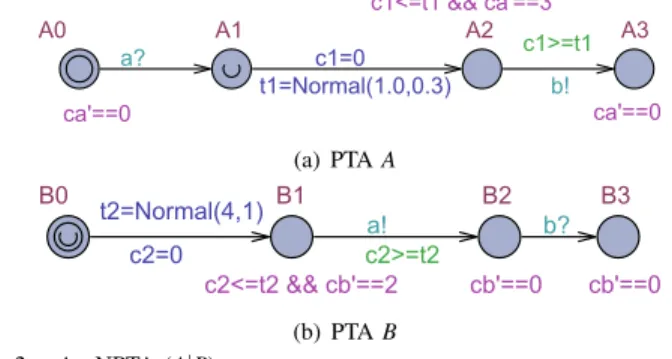
(b) PTA B Fig. 2. An NPTA (A|B)
Figure 2 shows an NPTA consisting of two PTAs A and B, where each PTA has four locations and two clocks (e.g., c1 and ca in A). The locations here marked with symbol
“U” are urgent locations which can freeze time. In other words, time is not allowed to pass when a PTA is in an urgent location [11]. Note that clocks can evolve with different rates (i.e., unit price) in different locations. The rate of a clock is 1 by default. To change the rate of a clock, we need to modify the rate value of the primed version of the clock. For example, c0a== 3 in A2 denotes that the rate
of ca is 3 in this location. Since UPPAAL-SMC supports
complex clock expression-based assignment for the primed clocks, UPPAAL-SMC can be used to model non-linear hybrid systems. Note that although UPPAAL-SMC only supports the uniform and exponential distributions explicitly, based on the C-like programming constructs and built-in function random() provided by UPPAAL-SMC various distributions can be constructed. For example, we can construct the normal distribution based on the Box-Muller approach [20]. Assume that the values of two variables t1 and t2 follow the normal
distributions N(1,0.32) and N(4,12), respectively. The action t 1=Normal(1,0.3)on the outgoing edge of A1assigns t1with
a random value following N(1,0.32). Since the invariant in A2 is c1 ≤ t1 and the guard on the outgoing edge of A2
is c1≥ t1, PTA A will be stuck at A2 for a time of t1.
If the NPTA is simulated for numerous times, the sojourn time at location A2 will follow the distribution N(1,0.32). In
action pairs (“!” indicating sending and “?” denotes receiving) via urgent channels a and b. While simulating (A|B) with a large number of runs, we can find that the reaching time of the composite location (A3, B3) follows the normal distri-bution N(4+1,12+ 0.32), since the sojourn time of (A|B) at composite locations (A0, B1) and (A2, B2) follows the normal distributions N(4,12)and N(1,0.32), respectively. By adopting the NPTA template like the above example, arbitrarily complex stochastic behaviors can be modeled.
2) Mapping from Uncertain Hybrid AADL to NPTA: To facilitate the detailed modeling of system architectures, AADL provides more types of syntax modeling constructs than NPTA. Since our approach focuses on quantitative analysis of stochastic behaviors of Uncertain Hybrid AADL designs, during the model transformation we neglect all the AADL constructs which cannot affect the system behaviors. Table I shows the structural mappings from uncertain Hybrid AADL constructs to NPTA constructs. Note that we only list a subset of AADL constructs that have a strong correlation with uncertainty-aware hybrid features. This subset can essentially be used to fully describe the behaviors of hybrid systems within an uncertain environment. In our approach, we use BLESS annex to specify the discrete components of systems, e.g., controller. We use the Hybrid annex to describe both discrete and continuous behaviors of hybrid components, e.g., plants. The instances of both annexes can be described using PTAs. Note that our proposed uncertainty annex focuses on the variation modeling of communication delays and parameter values. It only slightly changes structure of PTAs. To model the overall uncertain behaviors of the whole hybrid system, all the generated PTAs are synchronized through the channels, which are transformed from AADL connections.
TABLE I
CONSTRUCT MAPPINGS BETWEENAADLANDNPTA AADL Constructs NPTA Constructs
system (PTA1| . . . | PTAn)
thread / device PTA template (event) data port variable
connection urgent channel property set / type global variable BLESS annex subclause PTA template Hybrid annex subclause PTA template Uncertainty annex subclause PTA actions/invariants/guards
Our approach adopts the meta-models of AADL and its annexes to guide AADL model parsing as well as the con-struct mapping. Similar to the formal definitions presented in Section III-A, the meta-models define a set of correlated sub-constructs of the model, which can be used to extract the necessary information for the model transformation. Due to the space limit, we do not introduce the meta-models used in our approach here. The meta-model for the AADL without annex can be found in [4], and the meta-models for BLESS and Hybrid annexes can be obtained from [16] and [5], respectively. Similar to BLESS and Hybrid annex, the meta-model of Uncertainty annex can be inferred from Definition 3.4.
In our approach, the generated NPTA model can be divided into two parts: i) back-end configurations that are used to
declare necessary data structures (e.g., variables, channels) and functions (e.g., distributions, actions) for the stochastic mod-eling of NPTA modes, and ii) front-end models that are used to model the behaviors of hardware, software and environment components. Our approach assigns each of AADL components annotated by BLESS and Hybrid annex subclauses with a front-end model and a back-end configuration. Moreover, there is a global back-end configuration for the whole system whose information are shared by all the front-end models.
3) Back-end Configuration Generation: As a textual file, a back-end configuration mainly consists of: i) a set of decla-rations of variable and channels, and ii) a set of distribution and action functions. By using our approach, such information can be automatically extracted from AADL designs. Listing 2 shows the back-end configuration generated from the train AADL shown in Listing 1. To save the space, we put both the global configuration and the local configuration for the train within a same file.
For a back-end configuration, the global declarations of variable and channels are generated from the top level of AADL designs, i.e., hardware/software components and their interconnections. For each port of an AADL component, we create an urgent channel which indicates the AADL connec-tionassociated with the port. For example, assuming that the connection name bound by the port tv in the AADL design is tv, we will declare two things for this port in the global configuration. The first one is an urgent channel c tv that is used for the synchronization with other components. Since tv is a data port for the velocity of trains, we declare a variable v tv of type double to hold data value during the data transmission via the connection. The constants defined in the global NPTA configuration correspond to the constants (e.g., EOA) defined in top level of AADL designs. For each NPTA model, a clock systime is defined in the global configuration to model the system time. To model different stochastic behaviors of PTAs, the global back-end configuration comprises a library of distribution functions, which can be used by front-end NPTA models or the local configurations.
1 //global declarations & distribution function lib.
2 urgent chan c_tv, c_ts, c_ta; 3 double v_tv, v_ts, v_ta; 4 const double EOA=6000; 5 clock systime;
6 double Normal(double mean, double deviation){
7 // Box-Muller method
8 }
9 double Uniform(double min, double max){
10 ...
11 }
12 //local configuration for Train.
13 clock s, v, a, t, d_t; 14 double v_delay, fr;
15 void initialize(){
16 fr=Normal(-0.1,0.05);
17 }
18 //local configurations for other components.
19 ...
Listing 2. Back-end configuration of Train
The local back-end configuration mainly deals with the def-inition of data structures for specific AADL components and annexes. During the model transformation, all the continuous AADL variables are converted to clock typed variables, and
other AADL variables are converted to non-clock variables with different types. For each local configuration of PTAs, we define one built-in function initialize() which is used to initialize the values of variables. To enable the reset operation in a PTA, for each local configuration, we define one clock d t. For the uncertainty annex in Listing 1, there are two variables declared, i.e., v delay and v fr. Note that only v delay has a counterpart in the back-end configuration, since it is a time variable. The price variables have no counterparts, since they are used as intermediate variables during the model transformation. Note that the transformation rules for static and dynamic price variables are different. Since static price variables only take effect at the beginning of the simulation, we assign their random values to associated variables in the function initialize() of local back-end configurations. For example, we initialize the variable fr with a value following normal distribution N(−0.1, 0.052) in the back-end function
initialize() of the train example. Unlike static price variables, the dynamic price variables generate random values during the execution when necessary. It is widely used in front-end modeling to indicate the random value change of variables. For example, it can be used to model time-varying port delays.
4) Front-end Model Generation: As a graphical repre-sentation, front-end models are used in UPPAAL-SMC to describe the stochastic behaviors of PTAs. To describe the hybrid behaviors of systems, our approach adopts two kinds of annexes. We model the discrete behaviors of AADL com-ponents (e.g., thread component) using the BLESS annex. To describe continuous behaviors of components (e.g., device and abstract components), we use the Hybrid annex that is based on Hybrid CSP (Communicating Sequential Processes) [29]. For an AADL component without any annotated annexes, we assume a simplified semantics for its behavior, where the component periodically receives the data from its input ports and send the data to its output ports. Therefore, the major task of front-end model generation is to transform uncertainty-aware BLESS annexes and Hybrid annexes to their NPTA counterparts.
Uncertainty Modeling of Front-end Model: For front-end model transformation, we consider two kinds of uncertainties in the Uncertainty annex. The first one is described by time variables which are used to model the delay variations of network communication or task execution. To model such stochastic timing behaviors of system, we use the transforma-tion pattern as shown in Figure 3. Figure 3(a) shows a scenario that the PTA tries to send something via the channel using the action channel!. Without annotated Uncertainty annexes, the sending time of the action is fixed. However, by using our Uncertainty annex, we can associate a time variable v delay following normal distribution (i.e., N(1, 0.22)) with this chan-nel. By splitting the transition in Figure 3(a) and introducing a temporary location to indicate the waiting, we can model the model the scenario that the action time follows the N(1, 0.22) as shown in Figure 3(b). On the incoming edge of the newly added location temp, we assign v delay with a random value following N(1, 0.22) and we reset the clock d t. Since the invariant of location temp is d t<=v delay and the guard on the outgoing edge of temp is d t>=v delay. Therefore, the
PTA will stay at location temp for a time of v delay following the normal distribution N(1, 0.22). The second uncertainty in
the front-end model is specified by dynamic price variables in the uncertainty annex, which can mimic the random value of parameters (e.g., sensor inputs). The transformation of such uncertainty only needs to assign or replace the applied variable with the given distribution function.
(a) Certain (b) Uncertain Fig. 3. Transformation pattern for uncertain PTA models
BLESS Annex Based PTA Generation: The BLESS annex shares a large overlap of the modeling constructs with PTA. During the transformation, we can directly map the BLESS states to PTA locations. Since the definition of BLESS tran-sitions is more complex than the one of PTA trantran-sitions, we need to use some specific transformation patterns to generate PTA counterparts with equivalent semantics. In BLESS annex, a transition allows for a sequence of send (denoted by “!”) and receive (denoted by “?”) actions. However, PTA models only allow one of such actions on a transition. To model such combined send and receive actions, for each action on the BLESS transition, we introduce one temporary transition and one temporary location to trigger the action in the order of their occurrences on the BLESS transition. Note that there may be some time variable associated with the channel used by the send or receive actions. In this case, we need to introduce one more location together with one new transition to model the time delay of the action as the one shown in Figure 3. Moreover, BLESS annex provides assert section and invariant section to specify the behavior constraints of an AADL component. Such information can be directly parsed and used as the transition guards and location invariants in the generated PTA models.
Hybrid Annex Based PTA Generation: When transforming a Hybrid annex annotated AADL [5], the front-end PTA model is mainly extracted from the behavior section. Since Hybrid annex adopts the process algebra notations, the behavior of component is described by a set of CSP process, e.g., Train defined in the hybrid behavior section of Listing 1. During the transformation, each CSP process is converted to a location except for skip CSP process (e.g., Continue in Listing 1). The continuous evolution of a CSP process is expressed using differential expressions, which are translated and used as the invariant of the corresponding non-urgent location. As an example shown in Listing 1, the differential expression ’DT 1 s=v’indicates that the derivative of s is v. It can be translated into the derivative expression s’=v and used as a part of invariant for the location Train. To enable the communication between computation components and physic environments,
the semantics of Hybrid AADL allows two kinds of inter-ruptions, i.e., timed interrupts and communication interrupts. In the behavior section of Hybrid annex, a timed interrupt is defined as a part of CSP process in the form of [> time val] >, which will preempt the continuous evolution after an amount of time (i.e., time val). By using the similar transformation pattern shown in Figure 3, we can assure that the continuous evolution of CSP process can be interrupted after a time of time val. The communication interrupts enable the preemption of continuous evolutions by communication events via AADL ports. For example, the communication interrupt in the form of [[> pout!(v)]] > EV denotes that whenever a value of v is sent out the port pout, the current evolution will be terminated and the CSP process EV will be adopted as the subsequent behavior of the process. Generally, a communication interrupt may contain a sequence of send or receive actions. During the PTA transformation, we model the actions based on their occurrence order in the interrupt. For each action, we generate a new PTA location together with a new transition with the corresponding action on it. Note that in the generated PTA a location should be set as urgent if the action on next edge is a send action. When translating the choice operator of a CSP process, we will create a new adjacent location in the generated PTA for each alternative. The subsequent behavior of the process is determined by the Boolean expression associated with the alternative. To model the behavior of a repeating process defined in the behavior section, we connect the last location to the first location of the process in the PTA model to form a loop.
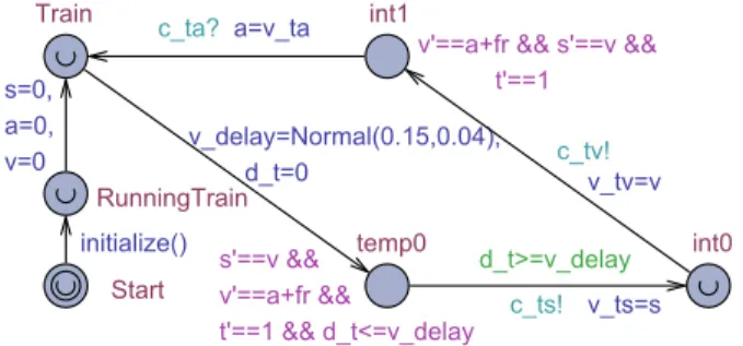
Fig. 4. PTA model of Train
Figure 4 shows the PTA of the Train example defined in the behavior section of Listing 1. To enable the exe-cution of function initialize() defined in the local back-end configuration, we introduce an urgent location start. On the outgoing transition of location RunningTrain, the continuous variables s, a and v are initialized. Since the first action in the communication interrupt is a send action (i.e., ts!(s)), we make the location Train urgent. As defined in the uncertainty annex, the channel associated with the port ts has a communication delay following N[0.15, 0.042]. Based on the pattern shown in Figure 3, we need to create a new location (i.e., temp0) to model the delay information. Note that ts is a data port, we need to sent the value of s via this port. However, the corresponding action c ts! on the outgoing edge of temp0 cannot hold the value information. Therefore we use the variable v ts which corresponds to the channel c ts to hold the data value during the communication via the channel. Since an
urgent location requires no invariants, we move the invariant derived from the different expression of CSP process Train to the new location temp0. Since there are three actions in the communication interrupt of the CSP process Train, we create two new locations to perform the actions according to their occurrence order. Note that the newly introduced three locations (i.e., temp0, int0 and int1) can be considered as the sub-locations of CSP process Train. Therefore, they should have the same location invariant. For the action ta?(a) of the communication interrupt, we need to get the data value from port ta. Therefore, we use the action a=v ta to update the value of a.
C. Property Generation for Quantitative Analysis
To enable the quantitative evaluation of Uncertain Hybrid AADL designs, our proposed Uncertainty annex allows de-signers to specify design requirements as performance queries. These performance queries will be transformed as properties in the form of cost-constrained temporal logic to reason the performance of the NPTA models generated from Uncertain Hybrid AADL designs. Since we focus on the reasoning of stochastic behaviors of AADL systems, the designers would like to conduct following two kinds of queries.
• Performance query: The performance query can be used to check the probability that an expected performance metric can be achieved under a given resource limit. The performance metric can be expressed as the predicate and the resource limit can be specified as the constraint using the keyword under.
• Safety query: The safety query can be used to check the probability that an unexpected scenario can happen eventually with a given resource limit. In the query, the unexpected scenario can be expressed as the predicate and the resource limit can be specified as the constraint using the keyword under.
Although safety queries and performance queries have different meaning, they share the same template during the property generation. In the queries section, a query consists of two parts, i.e., predicate φ and resource constraint ψ. The predicate φ can be used to denote either an unexpected scenario or an expected performance metric.
To evaluate the performance of generated NPTA models, UPPAAL-SMC adopts cost-constrained temporal logic [12] based performance queries in the form of Pr[bound](<> expr), where [bound] indicates the bound of the cost and the expression <> expr asserts that the scenario expr should happen eventually. By using our approach, the queries will be transformed into properties in the form of Pr[ψ](<> φ). For example, the performance query p2 in Listing 1 intends to check the probability that the travel length of the train exceeds 4 kilometers within 200 seconds. In order to conduct the quantitative evaluation using UPPAAL-SMC, the query will be converted to a property Pr[<= 200](<> Train.ts >= 4000) in the form of cost-constrained temporal logic. Based on the specified probability of false negatives (i.e., α) and probability uncertainty (i.e., ε), UPPAAL-SMC will simulate a specific number of stochastic runs which are terminated when either
bound or <> expr holds. The success rate p of <> expr satisfying bound will be reported in the form of a probability range [p − ε, p + ε] with a specified confidence 1 − α.
IV. CASESTUDY
To show the efficacy of our approach, this section presents the experimental results of verifying the Movement Authority (MA) control of Chinese Train Control System Level 3 (CTCS-3) [30], [21]. By using our proposed Uncertainty annex, we extended the hybrid CTCS-3 AADL model presented in [21] using the tool OSATE2 [6] based on the uncertainty information suggested by railway experts from our industrial partner. Based on our XMI parser and NPTA model generator implemented using JAVA1, we can obtain the corresponding NPTA model as well as performance queries. We employed the model checker UPPAAL-SMC (version 4.1.19, α = 0.02, ε = 0.02) to conduct the quantitative evaluation. All the experimental results were obtained on a desktop with 3.3GHz AMD CPU and 12GB RAM.
A. System Model of CTCS-3 MA Scenario
As one of the fourteen basic scenarios of CTCS-3 System Requirements Specification (SRS), the MA control plays an important role in prohibiting trains from colliding with each other. Typically an MA scenario involves three major compo-nents as follows: i) trains that are moving objects periodically (every 500 milliseconds) sending its status (i.e., current loca-tion and velocity) to the controller and receiving acceleraloca-tion information directed by the controller; ii) Radio Block Centers (RBCs) that provide MAs to trains based on information ex-change with trackside subsystems and the on-board controller; and iii) on-board controller subsystems which control the velocity of trains by changing their accelerations.
Radio Block Center
Movement
Authority EoA
SR
Fig. 5. MA scenario of CTCS-3 [21]
As shown in Figure 5, the RBC assigns a dynamic MA to the left train based on the track situation and the movement of the right train. Here, EOA stands for the End of Authorization. When a train reaches a specific distance (i.e., SR) away from EOA, it needs to apply for a new MA. If the authorization is not granted in time, according to SRS the train should stop before the EOA. According to SRS [30], an MA comprises
1We have shared our tool (including the source code of
Uncer-tain Hybrid AADL parser and NPTA model generator) and the un-certain CTCS-3 MA example on Github. The download address is https://github.com/tony11231/aadl2uppaal.
a sequence of segments, where each segment has two speed limits v1 and v2 (v1≥ v2). In this example, we set the speed
limits v1 and v2 for each segment to 73m/s and 66m/s,
respectively. If the train speed exceeds v1(v2), an emergency
(normal) brake will be performed to slow down the train. Upon receiving an MA request from controller, RBC will reply a new MA together with all the segment information (e.g., speed limits, operation mode). More details can be found in [30], [21]. In this example, we set the length of an MA to 6 kilometers, and set the length of SR to 1 kilometer. The train starts with a speed of 0m/s. All the segments have the same length and the speed limits. Note that within an uncertain environment, the SRS requirements cannot be guaranteed. For example, due to the mutual interference between varying com-munication delays and friction coefficient of tracks, inaccurate estimation of train location can make the train pass the EOA. Although train drivers can conduct emergency brake manually, proper quantitative analysis of these unsafe scenarios should be studied at architecture level to make the train movement more safe. pController pv ps pa Train tv ta ts pea pr
RBC
ea r m pm Controller cv ca r m cs ea 500ms conn_velocity conn_v conn_acc conn_a conn_position conn_s conn_ma conn_ma conn_ea conn_ea conn_req conn_reqFig. 6. AADL model for CTCS-3 MA
Figure 6 shows the graphical AADL model for CTCS-3 MA design, where the controller plays a central role. Within the MA scenario, the controller sends the MA request to RBC via the port r and receives the segment and EOA information from the ports m and ea, respectively. To achieve the train status, the controller receives the location and speed information from the ports cs and cv in every 500 milliseconds. It also controls the train by specifying the newly calculated acceleration for the train via port ca. Although this figure does not explicitly present any uncertainty information, in this example we consider various uncertainties that may affect the performance of the MA control, e.g., communication delays between RBC and controllers, computation time variations of both software/hardware components of controllers, and varied coefficient of friction of tracks. The cumulative variations by all these uncertainties strongly affect the performance and safety of the CTCS-3 MA. In other words, the risk of train collisions is high within an uncertain environment.
As shown in Table II, this experiment took nine uncertain aspects of CTCS-3 MA into consideration. Similar to the work in [28], [23], this paper adopts normal distributions to model the performance variations in the CTCS-3 MA scenario. All such variation information was collected from historical data of train operations. Note that our approach supports a variety of distributions, which can be used to accurately model the Uncertain Hybrid AADL designs. In this table,
the first column presents the category of the uncertainties. The second column presents the AADL constructs that cause the uncertainties. For example, when controller sends a MA request to RBC via port Controller.r, there is a delay variation caused by the connection conn req following the distribution N(0.1, 0.032), where the expected execution time is 0.1 second and the standard deviation is 0.03 second. Note that during the statistical model checking the network delay of 0.1 second with standard deviation of 0.03 may lead to a negative value. In our approach, if the variable with type “time” is randomly assigned with a negative value, we will set it to 0. According to the three-sigma rule [31], this approximation will still be accurate in this case. The last two columns provide the variation distributions and value unit, respectively. By using our tool chain, the NPTA model of the Uncertain Hybrid AADL design can be obtained automatically.
TABLE II
UNCERTAINTIES OFMA COMPONENTS Causes Constructs Variations Unit
Controller.r N(0.1, 0.032) Seconds
RBC.m N(0.1, 0.032) Seconds
Network RBC.ea N(0.1, 0.032) Seconds
Delay Train.tv N(0.15, 0.042) Seconds
Train.ts N(0.15, 0.042) Seconds
Controller.ca N(0.17, 0.042) Seconds
Parameter Train.fr N(−0.1, 0.052) MPSS∗
Execution RBC.T0 N(0.1, 0.032) Seconds
Time Controller.T5 N(0.2, 0.072) Seconds
*MPSS indicates Meter Per Second Squared.
B. Performance Analysis for CTCS-3 MA Scenario
To focus on quantitative analysis of the MA scenario influenced by uncertain factors, we investigated stochastic behaviors of a train within an MA as shown in Figure 5. We assume that the train will fail to get the next MA when entering SR. Therefore, it should stop before EOA. By using our tool, three queries are generated to analyze the performance of Uncertain Hybrid AADL design for CTCS-3 MA.
0 0.1 0.2 0.3 0.4 0.5 0.6 0.7 0.8 0.9 1 150 165 180 195 210 225 240 255 270 285 300 Probability Running Time
Cumulative Probability Distribution
a=0.3 MPSS a=0.4 MPSS a=0.7 MPSS
Fig. 7. Performance query results with different accelerations
To investigate the probability that a train can stop safely before the end of authorization within 300 seconds, we adopt the performance query Pr[<= 300](<> Train.v <= 0 && Train.s < 6000 && Train.s > 0), where Train.v denotes velocity of the train and Train.s indicates the location of the
train. Figure 7 presents the evaluation results for the query in the form of Cumulative Probability Distribution (CPD). In this figure, the x-axis denotes the time limit, and the y-axis indicates success rate of the performance requirement indicated by the query. In this evaluation, we considered three Uncertain Hybrid AADL designs, where the accelerations directed by the controller are different. We set the accelerations of three designs to 0.3 MPSS, 0.4 MPSS and 0.7 MPSS, respectively. By running 868 runs, we can get a probability interval [0.91,0.95] with a confidence 98% for the query of the AADL design with an acceleration of 0.3 MPSS. The SMC simulation for this query costs around 132 seconds. For the AADL designs with acceleration of 0.4 MPSS and 0.7 MPSS, we can get probability intervals [0.88,0.92] and [0.81,0.85] with a confidence of 98%, respectively. From this figure, we can find that the CPD of the design with 0.7 MPSS rises earlier (i.e., 173 seconds), since it has a larger acceleration and can reach the speed limit v2 more quickly
than the other two designs. However, the larger acceleration indicates the higher difficulty in managing the train speed. In other words, the chance that the train exceeds EOA becomes higher. Therefore, we can find that the AADL design with 0.3 MPSS can achieve the highest success rate to stop before reaching EOA. Moreover, we can find that the success rate will not increase significantly after a time threshold, since the train has stopped before the time limit, i.e., 300 seconds.
0 0.1 0.2 0.3 0.4 0.5 0.6 0.7 0.8 0.9 1 190 200 210 220 230 240 250 260 270 280 290 300 Probability Running Time
Cumulative Probability Distribution
st=0.2 S st=0.5 S st=0.7 S
Fig. 8. Performance query results with different control periods
The interaction frequency between trains and the controller plays an important role in CTCS-3 MA design, since it strongly affects the cost and performance of train designs. Although longer control periods cost less communication bandwidth, the infrequent updates of train accelerations make the train hard to be controlled. To investigate the effects of different control periods, we assume that the acceleration (without consider frictions) sent from the controller is fixed (i.e., 0.4 MPSS) for the train design. Figure 8 shows the evaluation results of using the same query as the one used in Figure 7. We consider three designs with different control periods, i.e., 0.2, 0.5 and 0.7 second, respectively. From this figure, we find that the design with the smallest control period (i.e., 0.2S) can achieve the highest rate of success. By running 266 runs, we can achieve a probability interval [0.95,0.99] with a confidence 98% for the query of the AADL design with a control periods of 0.2 second.
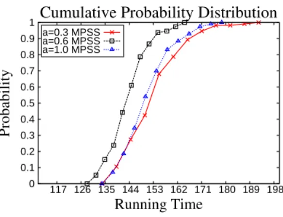
To determine the performance of the AADL design, we used the query Pr[<= 200](<> Train.s >= 4000) which checks whether the train can run a distance of 4.0 kilometers within 200 seconds. As shown in Figure 9, we adopted three designs with different accelerations. We can find that the performance difference among these three designs is quite small. The design with an acceleration of 0.3 MPSS achieves the worst performance, since it needs a worst-case time of 193 seconds to reach the specified location. Interestingly, the design with 1.0 MPSS does not win the comparison. It needs longer time to hit the specified location than the design with 0.6 MPSS, since the design with a larger acceleration will have a more drastic speed updates near the speed limits.
0 0.1 0.2 0.3 0.4 0.5 0.6 0.7 0.8 0.9 1 117 126 135 144 153 162 171 180 189 198 Probability Running Time
Cumulative Probability Distribution
a=0.3 MPSS a=0.6 MPSS a=1.0 MPSS
Fig. 9. Performance query results for reaching a location
C. Quantitative Safety Analysis for CTCS-3 MA Scenario During the running of the train, we do not expect the train speed exceeds the upper speed limit v1, since it can
easily make the train derailed. Therefore, when the train reaches the speed v1, we need to apply the urgent brake to
reduce the train speed drastically. To check the probability of overspeed of trains, we used the safety query in the form of Pr[Tran.s <= 5000](<> Train.v >= 73), which indicates that within a distance of |EOA − SR| the train speed cannot be larger than or equal to v1 (i.e., 73m/s). Figure 10 shows the
quantitative evaluation results for the three AADL designs with different accelerations. For the design with an acceleration of 0.3 MPSS, UPPAAL-SMC uses 17 seconds to obtain a probability interval [0.009, 0.049] for the query. From this figure, we can find that the larger the acceleration is, the higher chance the train can exceed the upper speed limit. To achieve a 2% chance of overspeed, the design with 1.0 MPSS needs an average travel distance of 3.0 kilometers, whereas the designs with 0.3 MPSS and 0.6 MPSS need an average of 3.5 kilometers and 4.1 kilometers, respectively.
V. CONCLUSIONS
Although there exist dozens of approaches for the analysis of AADL designs, most of them focus on the architectural correctness or the reachability analysis. Few of them support the performance analysis of AADL designs within uncertain environments. In this paper, we proposed a novel SMC-based framework that enables quantitative performance evaluation of Hybrid AADL designs considering various uncertain factors
0 0.01 0.02 0.03 0.04 0.05 0.06 0.07 0.08 0.09 0.1 3000 3300 3600 3900 4200 4500 Probability Running Distance
Cumulative Probability Distribution
a=0.3 MPSS a=0.6 MPSS a=1.0 MPSS
Fig. 10. Safety query results for overspeed
caused by physical environments. We introduced a lightweight language extension to AADL called Uncertainty annex for the stochastic behavior modeling. By using our proposed transformation rules, the uncertainty-aware Hybrid AADL designs can be automatically converted into NPTA models. Based on the statistical model checker UPPAAL-SMC, our framework enables automated evaluation of Uncertain Hybrid AADL designs against various complex performance and safety queries. Comprehensive experiment results carried on the CTCS-3 MA scenario demonstrate the feasibility and efficacy of our approach.
REFERENCES
[1] E. A. Lee, “Cyber Physical Systems: Design Challenges”, in in Pro-ceedings of International Symposium on Object Oriented Real-Time Distributed Computing (ISORC), 2008, pp. 363–369.
[2] P. Derler, E. A. Lee and A. Sangiovanni-Vincentelli, “Modeling Cyber-Physical Systems”, Proceedings of the IEEE, vol. 100, no. 1, pp. 13–28, 2012.
[3] P. H. Feiler and D. P. Gluch, “Model-Based Engineering with AADL: An Introduction to the SAE Architecture Analysis & Design Language”, Addison-Wesley, 2012.
[4] S. Aerospace, “SAE AS5506B: Architecture Analysis & Design Lan-guage (AADL) Standard Document”, SAE International, 2012. [5] E. Ahmad, B. R. Larson, S. C. Barrett, N. Zhan, and Y. Dong,
“Hybrid Annex: An AADL Extension for Continuous Behavior and Cyber-Physical Interaction Modeling”, in Proceedings of ACM Annual Conference on High Integrity Language Technology (HILT), 2014, pp. 29–38.
[6] OSATE2, http://osate.github.io/.
[7] K. Hu, T. Zhang, Z. Yang, and W.-T. Tsai, “Exploring AADL Verifi-cation Tool Through Model Transformation”, Journal of Systems Arch., vol. 61, no. 3, pp. 141–156, 2015.
[8] A. Johnsen, K. Lundqvist, P. Pettersson, and O. Jaradat, “Automated Verification of AADL-Specifications using UPPAAL”, in Proceedings of International Conference on High-Assurance Systems Engineering (HASE), 2012, pp. 130-138.
[9] K. G. Larsen, Priced Timed Automata and Statistical Model Checking. in Proceedings of International Conference on Integrated Formal Methods (IFM), 2013, pp. 154–161.
[10] P. Bulychev, A. David, K. G. Larsen, M. Mikucionis, D. B. Poulsen, A. Legay, and Z. Wang, “UPPAAL-SMC: Statistical Model Checking for Priced Timed Automata”, in Proceedings of International Workshop on Quantitative Aspects of Programming Languages and Systems (QAPL), 2012, pp. 1–16.
[11] A. David, K. G. Larsen, A. Legay, M. Mikucionis, and D. B. Poulsen, “UPPAAL SMC Tutorial”, International Journal on Software Tools for Technology Transfer (STTT), vol. 17, no. 4, pp. 1–19, 2015.


![Fig. 5. MA scenario of CTCS-3 [21]](https://thumb-eu.123doks.com/thumbv2/123doknet/13563352.420433/11.918.492.813.461.627/fig-ma-scenario-of-ctcs.webp)