HAL Id: hal-02976230
https://hal.archives-ouvertes.fr/hal-02976230
Submitted on 26 Oct 2020
HAL is a multi-disciplinary open access
archive for the deposit and dissemination of
sci-entific research documents, whether they are
pub-lished or not. The documents may come from
teaching and research institutions in France or
abroad, or from public or private research centers.
L’archive ouverte pluridisciplinaire HAL, est
destinée au dépôt et à la diffusion de documents
scientifiques de niveau recherche, publiés ou non,
émanant des établissements d’enseignement et de
recherche français ou étrangers, des laboratoires
publics ou privés.
and their terrestrial mechanisms for two types of El
Niños
Jun Wang, Ning Zeng, Meirong Wang, Fei Jiang, Jingming Chen, Pierre
Friedlingstein, Atul Jain, Ziqiang Jiang, Weimin Ju, Sebastian Lienert, et al.
To cite this version:
Jun Wang, Ning Zeng, Meirong Wang, Fei Jiang, Jingming Chen, et al.. Contrasting interannual
atmospheric CO2 variabilities and their terrestrial mechanisms for two types of El Niños. Atmospheric
Chemistry and Physics, European Geosciences Union, 2018, 18 (14), pp.10333-10345.
�10.5194/acp-18-10333-2018�. �hal-02976230�
https://doi.org/10.5194/acp-18-10333-2018 © Author(s) 2018. This work is distributed under the Creative Commons Attribution 4.0 License.
Contrasting interannual atmospheric CO
2
variabilities and their
terrestrial mechanisms for two types of El Niños
Jun Wang1,2, Ning Zeng2,3, Meirong Wang4, Fei Jiang1, Jingming Chen1,5, Pierre Friedlingstein6, Atul K. Jain7, Ziqiang Jiang1, Weimin Ju1, Sebastian Lienert8,9, Julia Nabel10, Stephen Sitch11, Nicolas Viovy12, Hengmao Wang1, and Andrew J. Wiltshire13
1International Institute for Earth System Science, Nanjing University, Nanjing, China
2State Key Laboratory of Numerical Modelling for Atmospheric Sciences and Geophysical Fluid Dynamics,
Institute of Atmospheric Physics, Beijing, China
3Department of Atmospheric and Oceanic Science and Earth System Science Interdisciplinary Center,
University of Maryland, College Park, Maryland, USA
4Joint Center for Data Assimilation Research and Applications/Key Laboratory of Meteorological Disaster of Ministry of
Education, Nanjing University of Information Science & Technology, Nanjing, China
5Department of Geography, University of Toronto, Toronto, Ontario M5S3G3, Canada
6College of Engineering, Mathematics and Physical Sciences, University of Exeter, Exeter, EX4 4QF, UK 7Department of Atmospheric Sciences, University of Illinois at Urbana-Champaign, Urbana, IL 61801, USA 8Climate and Environmental Physics, Physics Institute, University of Bern, Bern, Switzerland
9Oeschger Centre for Climate Change Research, University of Bern, Bern, Switzerland 10Land in the Earth System, Max Planck Institute for Meteorology, 20146 Hamburg, Germany 11College of Life and Environmental Sciences, University of Exeter, Exeter, EX4 4RJ, UK
12Laboratoire des Sciences du Climat et de l’Environnement, LSCE/IPSL-CEA-CNRS-UVQS, 91191, Gif-sur-Yvette, France 13Met office Hadley Centre, FitzRoy Road, Exeter, EX1 3PB, UK
Correspondence: Ning Zeng (zeng@umd.edu) and Fei Jiang (jiangf@nju.edu.cn) Received: 25 February 2018 – Discussion started: 13 March 2018
Revised: 19 June 2018 – Accepted: 5 July 2018 – Published: 19 July 2018
Abstract. El Niño has two different flavors, eastern Pa-cific (EP) and central PaPa-cific (CP) El Niños, with different global teleconnections. However, their different impacts on the interannual carbon cycle variability remain unclear. Here we compared the behaviors of interannual atmospheric CO2
variability and analyzed their terrestrial mechanisms during these two types of El Niños, based on the Mauna Loa (MLO) CO2 growth rate (CGR) and the Dynamic Global
Vegeta-tion Model’s (DGVM) historical simulaVegeta-tions. The composite analysis showed that evolution of the MLO CGR anomaly during EP and CP El Niños had three clear differences: (1) negative or neutral precursors in the boreal spring during an El Niño developing year (denoted as “yr0”), (2) strong or weak amplitudes, and (3) durations of the peak from Decem-ber (yr0) to April during an El Niño decaying year (denoted as “yr1”) compared to October (yr0) to January (yr1) for a
CP El Niño, respectively. The global land–atmosphere car-bon flux (FTA) simulated by multi-models was able to
cap-ture the essentials of these characteristics. We further found that the gross primary productivity (GPP) over the tropics and the extratropical Southern Hemisphere (Trop + SH) gen-erally dominated the global FTA variations during both El
Niño types. Regional analysis showed that during EP El Niño events significant anomalous carbon uptake caused by in-creased precipitation and colder temperatures, correspond-ing to the negative precursor, occurred between 30◦S and 20◦N from January (yr0) to June (yr0). The strongest anoma-lous carbon releases, largely due to the reduced GPP induced by low precipitation and warm temperatures, occurred be-tween the equator and 20◦N from February (yr1) to August (yr1). In contrast, during CP El Niño events, clear carbon releases existed between 10◦N and 20◦S from September
(yr0) to September (yr1), resulting from the widespread dry and warm climate conditions. Different spatial patterns of land temperatures and precipitation in different seasons as-sociated with EP and CP El Niños accounted for the evolu-tionary characteristics of GPP, terrestrial ecosystem respira-tion (TER), and the resultant FTA. Understanding these
dif-ferent behaviors of interannual atmospheric CO2variability,
along with their terrestrial mechanisms during EP and CP El Niños, is important because the CP El Niño occurrence rate might increase under global warming.
1 Introduction
The El Niño–Southern Oscillation (ENSO), a dominant year-to-year climate variation, leads to a significant interannual variability in the atmospheric CO2growth rate (CGR)
(Ba-castow, 1976; Keeling et al., 1995). Many studies, including measurement campaigns (Lee et al., 1998; Feely et al., 2002), atmospheric inversions (Bousquet et al., 2000; Peylin et al., 2013), and terrestrial carbon cycle models (Zeng et al., 2005; Wang et al., 2016), have consistently suggested the dominant role of terrestrial ecosystems, especially tropical ecosystems, in contributing to interannual atmospheric CO2 variability.
Recently, Ahlstrom et al. (2015) further suggested ecosys-tems over the semi-arid regions played the most important role in the interannual variability of the land CO2sink.
More-over, this ENSO-related interannual carbon cycle variability may be enhanced under global warming, with approximately a 44 % increase in the sensitivity of terrestrial carbon flux to ENSO (Kim et al., 2017).
Tropical climatic variations (especially in surface air tem-perature and precipitation) induced by ENSO and plant and soil physiological responses can largely account for interan-nual terrestrial carbon cycle variability (Zeng et al., 2005; Wang et al., 2016; Jung et al., 2017). Multi-model simu-lations involved in the TRENDY project and the Coupled Model Intercomparison Project Phase 5 (CMIP5) have con-sistently suggested the biological dominance of gross pri-mary productivity (GPP) or net pripri-mary productivity (NPP) (Kim et al., 2016; Wang et al., 2016; Piao et al., 2013; Ahlstrom et al., 2015). However, debates continue regard-ing which is the dominant climatic mechanism (temperature or precipitation) in the interannual variability of the terres-trial carbon cycle (Wang et al., 2013, 2014, 2016; Cox et al., 2013; Zeng et al., 2005; Ahlstrom et al., 2015; Qian et al., 2008; Jung et al., 2017).
The atmospheric CGR or land–atmosphere carbon flux (FTA – if this is positive, this indicates a flux into the
at-mosphere) can anomalously increase during El Niño and de-crease during La Niña episodes (Zeng et al., 2005; Keeling et al., 1995). Cross-correlation analysis shows that the atmo-spheric CGR and FTAlag the ENSO by several months (Qian
et al., 2008; Wang et al., 2013, 2016). This is due to the
period needed for surface energy and soil moisture adjust-ment following ENSO-related circulation and precipitation anomalies (Gu and Adler, 2011; Qian et al., 2008). How-ever, considering the variability inherent in the ENSO phe-nomenon (Capotondi et al., 2015), the atmospheric CGR and FTA can show different behaviors during different El Niño
events (Schwalm, 2011; Wang et al., 2018).
El Niño events can be classified into eastern Pacific El Niño (EP El Niño, also termed as conventional El Niño) and central Pacific El Niño (CP El Niño, also termed as El Niño Modoki) according to the patterns of sea surface warming over the tropical Pacific (Ashok et al., 2007; Ashok and Ya-magata, 2009). These two types of El Niño have different global climatic teleconnections, associated with contrasting climate conditions in different seasons (Weng et al., 2007, 2009). For example, positive winter temperature anomalies are located mostly over the northeastern US during an EP El Niño, while warm anomalies occur in the northwestern US during a CP El Niño (Yu et al., 2012). The contrasting summer and winter precipitation anomaly patterns associ-ated with these two El Niño events over China, Japan, and the US were also discussed by Weng et al. (2007, 2009). Im-portantly, Ashok et al. (2007) suggested that the occurrence of the CP El Niño had increased during recent decades com-pared to the EP El Niño. This phenomenon can probably be attributed to the anthropogenic global warming (Ashok and Yamagata, 2009; Yeh et al., 2009).
However, the contrasting impacts of EP and CP El Niño events on carbon cycle variability remain unclear. In this study, we attempt to reveal their different impacts given the different regional responses of the EP and CP El Niños. We compared the behavior of interannual atmospheric CO2
vari-ability and analyzed their terrestrial mechanisms correspond-ing to these two types of El Niños, based on Mauna Loa (MLO) long-term CGR and TRENDY multi-model simula-tions.
This paper is organized as follows: Sect. 2 describes the datasets used, methods, and TRENDY models selected. Sec-tion 3 reports the results regarding the relaSec-tionship between ENSO and CGR and EP and CP El Niño events, in addition to a composite analysis on carbon cycle behaviors, and ter-restrial mechanisms. Section 4 contains a discussion of the results, and Sect. 5 presents concluding remarks.
2 Datasets and methods 2.1 Datasets used
Data for monthly atmospheric CO2concentrations between
1960 and 2013 were collected from the National Oceanic and Atmospheric Administration (NOAA) Earth System Re-search Laboratory (ESRL) (Thoning et al., 1989). The an-nual CO2growth rate (CGR) in Pg C yr−1was derived month
(a)
(b)
flux
Niño
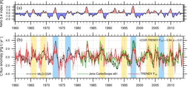
Figure 1. Interannual variability in the Niño3.4 index and the carbon cycle. (a) Niño3.4. (b) Mauna Loa (MLO) CO2growth rate (CGR, black line), as well as TRENDY multi-model median (red line) and Jena inversion (green line) of the global land–atmosphere carbon flux (FTA; a positive value means flux into the atmosphere; units: Pg C yr−1), which were further smoothed by the 3-month running average. The
light red shading represents the area between the 5 and 95 % percentiles of the TRENDY simulations. The bars represent the El Niño events selected for this study, with the EP El Niño in blue and the CP El Niño in yellow.
al. (2005) and Sarmiento et al. (2010). The calculation is as follows:
CGR (t ) = γ · [pCO2(t +6) − pCO2(t −6)], (1)
where γ = 2.1276 Pg C ppm−1, pCO2 is the atmospheric
partial pressure of CO2in ppm, and t is the time in months.
The detailed calculation of the conversion factor, γ , can be found in the appendix of Sarmiento et al. (2010).
Temperature and precipitation datasets for 1960 through 2013 were obtained from CRUNCEPv6 (Wei et al., 2014). CRUNCEP datasets are the merged product of ground observation-based CRU data and model-based NCEP– NCAR Reanalysis data with a 0.5◦×0.5◦spatial resolution and 6 h temporal resolution. These datasets are consistent with the climatic forcing used to run dynamic global vegeta-tion models in TRENDY v4 (Sitch et al., 2015). The sea sur-face temperature anomalies (SSTAs) over the Niño3.4 region (5◦S–5◦N, 120–170◦W) were obtained from the NOAA’s Extended Reconstructed Sea Surface Temperature (ERSST) dataset, version 4 (Huang et al., 2015).
The inversion of FTAfrom the Jena CarboScope was used
for comparison with the TRENDY multi-model simulations from 1981 to 2013. The Jena CarboScope Project provided the estimates of the surface–atmosphere carbon flux based on atmospheric measurements using an “atmospheric trans-port inversion”. The inversion run used here was s81_v3.8 (Rodenbeck et al., 2003).
2.2 TRENDY simulations
We analyzed eight state-of-the-art dynamic global vegeta-tion models from TRENDY v4 for the period 1960–2013:
CLM4.5 (Oleson et al., 2013), ISAM (Jain et al., 2013), JS-BACH (Reick et al., 2013), JULES (Clark et al., 2011), LPX-Bern (Keller et al., 2017), OCN (Zaehle and Friend, 2010), VEGAS (Zeng et al., 2005), and VISIT (Kato et al., 2013) (Table 1). Since LPX-Bern was excluded in the analysis of TRENDY v4, due to it not fulfilling the minimum perfor-mance requirement, the output over the same time period of a more recent, better performing version (LPX-Bern v1.3) was used. These models were forced using a common set of cli-matic datasets (CRUNCEPv6), and followed the same exper-imental protocol. Models use different vegetation datasets or internally generated vegetation. The S3 run was used in this study, in which simulations were forced by all the drivers, in-cluding CO2, climate, land use, and land cover change (Sitch
et al., 2015).
The simulated terrestrial variables (net biome produc-tivity (NBP), GPP, terrestrial ecosystem respiration (TER), soil moisture, and others) were interpolated into a consis-tent 0.5◦×0.5◦resolution using the first-order conservative remapping scheme (Jones, 1999) by Climate Data Operators (CDO): Fk= 1 Ak Z fdA, (2)
where Fkdenotes the area-averaged destination quantity, Ak
is the area of cell k, and f is the quantity in an old grid which has an overlapping area with the destination grid. Then the median, 5, and 95 % percentiles of the multi-model simula-tions were calculated grid by grid to study the different ef-fects of EP and CP El Niños on terrestrial carbon cycle inter-annual variability.
(a) EP El Niño (b) CP El Niño
Figure 2. Schematic diagram of the two types of El Niños. (a) Sea surface temperature anomaly (SSTA) over the tropical Pacific associated with the anomalous Walker circulation in an EP El Niño. (b) SSTA with two cells of the anomalous Walker circulation in a CP El Niño. Red colors indicate warming, and blue colors indicate cooling. Vectors denote the wind directions.
yr0 yr1 yr0 yr1
Niño
Niño
flux
flux
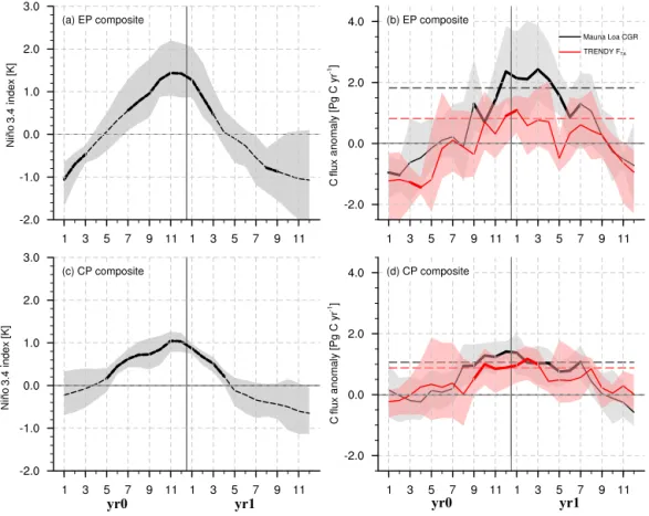
Figure 3. Composites of El Niño and the corresponding carbon flux anomaly (Pg C yr−1). (a) The Niño3.4 index composite during EP El Niño events. (b) Corresponding MLO CGR and TRENDY v4 global FTAcomposite during EP El Niño events. (c) The Nino3.4 index
composite during CP El Niño events. (d) Corresponding MLO CGR and TRENDY v4 global FTAcomposite during CP El Niño events. The
shaded area denotes the 95 % confidence intervals of the variables in the composite, derived from 1000 bootstrap estimates. The bold lines indicate the significance above the 80 % level estimated by the Student’s t test. The black and red dashed lines in (b) and (d) represent the thresholds of the peak duration (75 % of the maximum CGR or FTAanomaly).
2.3 El Niño criterion and classification methods El Niño events are determined by the Oceanic Niño Index (ONI) (i.e., the running 3-month mean SST anomaly over
Table 1. TRENDY models used in this study.
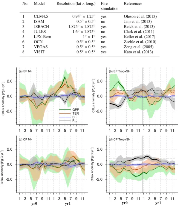
No. Model Resolution (lat × long.) Fire References simulation
1 CLM4.5 0.94◦×1.25◦ yes Oleson et al. (2013) 2 ISAM 0.5◦×0.5◦ no Jain et al. (2013) 3 JSBACH 1.875◦×1.875◦ yes Reick et al. (2013) 4 JULES 1.6◦×1.875◦ no Clark et al. (2011) 5 LPX-Bern 1◦×1◦ yes Keller et al. (2017) 6 OCN 0.5◦×0.5◦ no Zaehle et al. (2010) 7 VEGAS 0.5◦×0.5◦ yes Zeng et al. (2005) 8 VISIT 0.5◦×0.5◦ yes Kato et al. (2013)
yr0 yr1 yr0 yr1
flux
flux
flux
flux
Figure 4. Composites of anomalies in the TRENDY FTA(black lines), gross primary productivity (GPP, green lines), terrestrial ecosystem
respiration (TER, brown lines), and the carbon flux caused by disturbances (D, blue lines) during two types of El Niños over the extratropical Northern Hemisphere (NH, 23–90◦N) and the tropics and extratropical Southern Hemisphere (Trop + SH, 60–23◦S). The shaded area denotes the 95 % confidence intervals of the variables in the composite, derived from 1000 bootstrap estimates. The bold lines indicate the significance above the 80 % level estimated by the Student’s t test. The black dashed lines in b and d represent the thresholds of the peak duration.
the Niño3.4 region; Fig. 1a). This NOAA criterion is that El Niño events are defined as five consecutive overlapping 3-month periods at or above the +0.5◦anomaly.
We classified El Niño events into EP or CP based on the consensus of three different identification methods directly adopted from a previous study (Yu et al., 2012). These iden-tification methods included the El Niño Modoki Index (EMI)
(Ashok et al., 2007), the EP/CP index method (Kao and Yu, 2009), and the Niño method (Yeh et al., 2009).
2.4 Anomaly calculation and composite analysis To calculate the anomalies, we first removed the long-term climatology for the period from 1960 to 2013 from all of the variables used here, both modeled and observed, in order to
eliminate the seasonal cycle. We then detrended them based on a linear regression because (1) the trend in terrestrial car-bon variables was mainly caused by long-term CO2
fertiliza-tion and climate change, and (2) the trend in CGR primarily resulted from the anthropogenic emissions. We used these detrended monthly anomalies to investigate the impacts of El Niño events on the interannual carbon cycle variability.
More specifically, in terms of the composite analysis, we calculated the averages of the carbon flux anomaly (CGR, FTAetc.) during the selected EP and CP El Niño events,
re-spectively. We use the bootstrap methods (Mudelsee, 2010) to estimate the 95 % confidence intervals and the Student’s ttest to estimate the significance levels in the composite anal-ysis. An 80 % significance level was selected, as per Weng et al. (2007), due to the limited number of EP El Niño events.
3 Results
3.1 The relationship between ENSO and interannual atmospheric CO2variability
The interannual atmospheric CO2variability closely coupled
with ENSO (Fig. 1) with noticeable increases in CGR during El Niño and decreases during La Niña, respectively (Bacas-tow, 1976; Keeling and Revelle, 1985). The correlation coef-ficient between the MLO CGR and the Niño3.4 index from 1960 to 2013 was 0.43 (p < 0.01). A regression analysis fur-ther indicated that a per unit increase in the Niño3.4 index can lead to a 0.60 Pg C yr−1increase in the MLO CGR.
The variation in the global FTA anomaly simulated by
TRENDY models resembled the MLO CGR variation, with a correlation coefficient of 0.54 (p < 0.01; Fig. 1b). This was close to the correlation coefficient of 0.61 (p < 0.01; Fig. 1b) between the MLO CGR and the Jena CarboScope s81 for the time period from 1981 to 2013. This indicates that the ter-restrial carbon cycle can largely explain the interannual at-mospheric CO2variability, as suggested by previous studies
(Bousquet et al., 2000; Zeng et al., 2005; Peylin et al., 2013; Wang et al., 2016). Moreover, the correlation coefficient of the TRENDY global FTAand the Niño3.4 index reached 0.49
(p < 0.01), and a similar regression analysis of FTA with
Niño3.4 showed a sensitivity of 0.64 Pg C yr−1K−1. How-ever, owing to the diffuse light fertilization effect induced by the eruption of Mount Pinatubo in 1991 (Mercado et al., 2009), the Jena CarboScope s81 indicated that the terrestrial ecosystems had an anomalous uptake during the 1991–1992 El Niño event, making the MLO CGR an anomalous de-crease. However, TRENDY models did not capture this phe-nomenon. This was not only due to a lack of a corresponding process representation in some models, but also because the TRENDY protocol did not include diffuse and direct light forcing.
Table 2. Eastern Pacific (EP) and central Pacific (CP) El Niño events used in this study, as identified by a majority consensus of three methods. EP El Niño CP El Niño 1972–1973 1965–1966 1976–1977 1968–1969 1997–1998 1987–1988 2006–2007 1994–1995 2002–2003 2004–2005 2009–2010
3.2 EP and CP El Niño events
Schematic diagrams of the two types of El Niños (EP and CP) are shown in Fig. 2. During EP El Niño events (Fig. 2a), a positive sea surface temperature anomaly (SSTA) occurs in the eastern equatorial Pacific Ocean, showing a dipole SSTA pattern with the positive zonal SST gradient. This condition forms a single cell of Walker circulation over the tropical Pa-cific, with a dry downdraft in the western Pacific and wet updraft in the central-eastern Pacific. In contrast, an lous warming in the central Pacific, sandwiched by anoma-lous cooling in the east and west, is observed during CP El Niño events (Fig. 2b). This tripole SSTA pattern makes the positive/negative zonal SST gradient in the western/eastern tropical Pacific, resulting in an anomalous two-cell Walker circulation over the tropical Pacific. This alteration in atmo-spheric circulation produces a wet region in the central Pa-cific. Moreover, apart from these differences in the equato-rial Pacific, the SSTA in other oceanic regions also differs remarkably (Weng et al., 2007, 2009).
Based on the NOAA criterion, a total of 17 El Niño events were detected from 1960 through 2013. The events were then categorized into an EP or a CP El Niño based on a con-sensus of three identification methods (EMI, EP/CP index, and Niño methods) (Yu et al., 2012). Considering the effect of diffuse radiation fertilization induced by volcano erup-tions (Mercado et al., 2009), we removed the 1963–1964, 1982–1983, and 1991–1992 El Niño events, in which Mount Agung, El Chichón, and Pinatubo erupted, respectively. In addition, we closely examined those extended El Niño events that occurred in 1968–1970, 1976–1978, and 1986–1988. Based on the typical responses of MLO CGR to El Niño events (anomalous increase lasting from the El Niño devel-oping year to El Niño decaying year; Supplement Fig. S1), we retained 1968–1969, 1976–1977, and 1987–1988 El Niño periods. Finally, we obtained four EP El Niño and seven CP El Niño events in this study (Table 2; Fig. 1b and Supplement Fig. S2), with the composite SSTA evolutions as shown in the Supplement Fig. S3.
yr0 yr1 yr0 yr1
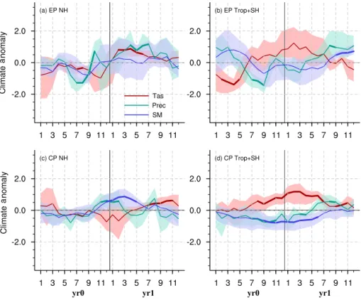
Figure 5. Composites of the standardized land surface air temperature (Tas, red lines), precipitation (green lines), and TRENDY-simulated soil moisture content (SM, blue lines) anomalies in two types of El Niños over the NH and over Trop + SH. The shaded area denotes the 95 % confidence intervals of the variables in the composite, derived from 1000 bootstrap estimates. The bold lines indicate the significance above the 80 % level estimated by the Student’s t test.
3.3 Responses of atmospheric CGR to two types of El Niños
Based on the selected EP and CP El Niño events, a compos-ite analysis was conducted with the non-smoothed detrended monthly anomalies of the MLO CGR and the TRENDY global FTAto reveal the contrasting carbon cycle responses
to these two types of El Niños (Fig. 3). In addition to the differences in the location of anomalous SST warming and the alteration of the atmospheric circulation in EP and CP El Niños shown in Fig. 2, the following findings were eluci-dated.
1. Different El Niño precursors. The SSTA was signifi-cantly negative in the EP El Niño during the boreal win-ter (JF) and spring (MAM) in yr0 (hereafwin-ter “yr0” and “yr1” refer to the El Niño developing and decaying year, respectively). Conversely, the SSTA was neutral in the CP El Niño.
2. Different tendencies of SST (∂SST /∂t ). The tendency of SST in the EP El Niño was stronger than that in the CP El Niño.
3. Different El Niño amplitudes. Due to the different ten-dencies of SST, the amplitude of the EP El Niño was
basically stronger than that of the CP El Niño, though they all reached maturity in November or December of yr0 (Fig. 3a and c).
Correspondingly, behaviors of the MLO CGR during these two types of El Niño events also displayed some differ-ences (Fig. 3b and d). During EP El Niño events (Fig. 3b), the MLO CGR was negative in boreal spring (yr0) and in-creased quickly from boreal fall (yr0), whereas it was neu-tral in boreal spring (yr0) and slowly increases from boreal summer (yr0) during the CP El Niño episode (Fig. 3d). The amplitude of the MLO CGR anomaly during EP El Niño events was generally larger than that during CP El Niño events. Importantly, the duration of the MLO CGR peak dur-ing EP El Niño was from December (yr0) to April (yr1), while the MLO CGR anomaly peaked from October (yr0) to January (yr1) during CP El Niño. Here we simply defined the peak duration as the period above the 75 % of the maximum CGR (or FTA) anomaly, in which the variabilities of less than
3 months below the threshold were also included. The pos-itive MLO CGR anomaly ended around September (yr1) in both cases (Fig. 3b and d). During the finalization of this pa-per, we noted the publication of Chylek et al. (2018) who also found a CGR amplitude difference in response to the two types of events.
yr0 yr1 yr0 yr1 yr0 yr1
p t
p t
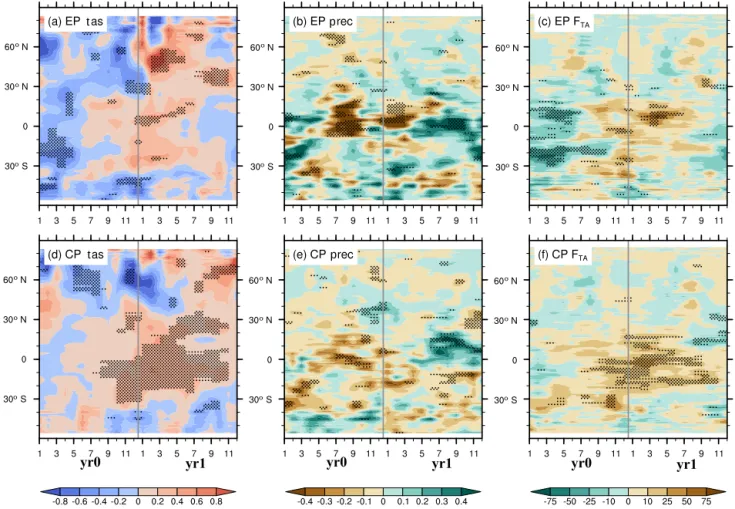
Figure 6. Hovmöller diagrams of the anomalies in climate variables and the FTA(averaged from 180◦W to 180◦E) during EP and CP El
Niño events. Panels (a and d) show surface air temperature anomalies over land (units: K); panels (b and e) show precipitation anomalies over land (units: mm d−1); panels (c and f) show TRENDY-simulated FTAanomalies (units: g C m−2yr−1) during EP and CP El Niño events.
The dotted areas indicate the significance above the 80 % level as estimated using the Student’s t test.
A comparison of the MLO CGR with the TRENDY global FTA anomalies (Fig. 3b and d) indicated that the TRENDY
global FTA effectively captured the characteristics of CGR
evolution during the CP El Niño. In contrast, the amplitude of the TRENDY global FTAanomaly was somewhat
under-estimated during the EP El Niño, causing a lower statisti-cal significance (Fig. 3b). This underestimation of the global FTAanomaly can, for example, be clearly seen in a
compar-ison between the TRENDY and the Jena CarboScope during the extreme 1997–1998 EP El Niño (Fig. 1b). Also, other characteristics can be basically captured. Therefore, insight into the mechanisms of these CGR evolutions during EP and CP El Niños, based on the simulations by TRENDY models, is still possible.
3.4 Regional contributions, characteristics, and their mechanisms
We separated the TRENDY global FTA anomaly by major
geographic regions into two parts: the extratropical
North-ern Hemisphere (NH, 23◦N–90◦N), and the tropics plus ex-tratropical Southern Hemisphere (Trop + SH, 60◦S–23◦N) (Fig. 4). In a comparison of the contributions from these two parts, it was found that the FTA over Trop + SH played a
more important role in the global FTAanomaly in both cases
(Fig. 4b and d), and this finding was consistent with previous studies (Bousquet et al., 2000; Peylin et al., 2013; Zeng et al., 2005; Wang et al., 2016; Ahlstrom et al., 2015; Jung et al., 2017). The FTAover Trop + SH was negative in austral fall
(MAM; yr0), increased from austral spring (SON; yr0), and peaked from December (yr0) to April (yr1) during the EP El Niño (Fig. 4b). Conversely, it was nearly neutral in aus-tral fall (yr0), increased from ausaus-tral winter (JJA; yr0), and peaked from November (yr0) to March (yr1) during the CP El Niño (Fig. 4d). These evolutionary characteristics in the FTA over the Trop + SH were generally consistent with the
global FTA and the MLO CGR (Fig. 3b and d). In contrast,
the contributions from the FTA anomaly over the NH were
According to the equation FTA= −NBP = TER − GPP +
D (where D is the carbon flux caused by disturbances such as wildfires, harvests, grazing, and land cover change), the variation in FTAcan be explained by the variations in GPP,
TER, and D. The D simulated by TRENDY was nearly neu-tral during both El Niño types (Fig. 4). Therefore, GPP and TER largely accounted for the variation in FTA.
More specifically, in Trop + SH, GPP anomalies domi-nated the variations in FTAfor both El Niño types, but their
evolutions differed (Fig. 4b and d). The GPP showed an anomalous positive value during austral fall (yr0), and an anomalous negative value from austral fall (yr1) to winter (yr1), with the minimum around April (yr1) during the EP El Niño (Fig. 4b). Conversely, the GPP anomaly was always negative, with the minimum occurring around October or November (yr0) during the CP El Niño (Fig. 4d). The varia-tion in the TER in both El Niños was relatively weaker than that of the GPP (Fig. 4b and d). The anomalous positive TER during austral spring (yr0) and summer (yr1) accounted for the increase in FTA, and it partly canceled the negative GPP
in austral fall (yr1) and winter (yr1) during the EP El Niño (Fig. 4b). In contrast, the TER had a reduction in yr0 dur-ing the CP El Niño (Fig. 4d). Over the NH, though the FTA
anomaly was relatively weaker, the behaviors of GPP and TER differed in EP and CP El Niños. GPP and TER consis-tently decreased in the growing season of yr0 and increased in the growing season of yr1 during the EP El Niño (Fig. 4a), whereas they only showed some increase during boreal sum-mer (yr1) during the CP El Niño (Fig. 4c).
These evolutionary characteristics of GPP, TER, and the resultant FTA principally resulted from their responses to
the climate variability. Figure 5 shows the standardized ob-served surface air temperature, precipitation, and TRENDY-simulated soil moisture contents. Over the Trop + SH, taking into consideration the regulation of thermodynamics and the hydrological cycle on the surface energy balance, variations in temperature and precipitation (soil moisture) were always opposite during the two types of El Niños (Fig. 5b and d). Additionally, adjustments in soil moisture lagged precipita-tion by approximately 2–4 months, owing to the so-called “soil memory” of water recharge (Qian et al., 2008). The variations in GPP in both the El Niño types were closely as-sociated with variations in soil moisture, namely water avail-ability largely dominated by precipitation (Figs. 4b, d and 5b, d), and this result was consistent with previous studies (Zeng et al., 2005; Zhang et al., 2016). Warm temperatures during El Niño episodes can enhance the ecosystem respi-ration, but dry conditions can reduce it. These cancelations from warm and dry conditions made the amplitude of TER variation smaller than that of GPP (Fig. 4b and d). Over the NH, variations in temperature and precipitation were basi-cally in the same direction (Fig. 5a and c), as opposed to their behaviors over the Trop + SH. This was due to the differ-ent climatic dynamics of the two regions (Zeng et al., 2005). During the EP El Niño event, cool and dry conditions in the
boreal summer (yr0) inhibited GPP and TER, whereas warm and wet conditions in the boreal spring and summer (yr1) enhanced them (Figs. 5a and 4a). In contrast, only the warm and wet conditions in boreal summer (yr1) enhanced GPP and TER during the CP El Niño event (Figs. 5c and 4c). These different configurations of temperature and precipita-tion variaprecipita-tions during EP and CP El Niños form the different evolutionary characteristics of GPP, TER, and the resultant FTA.
Detailed regional evolutionary characteristics can be seen from the Hovmöller diagrams in Fig. 6 and in the Supple-ment Figs. S4 and S5. Obvious large anomalies in FTA
con-sistently occurred from 20◦N to 40◦S during EP and CP El Niños (Fig. 6c and f), consistent with the above analyses (Fig. 4b and d). Moreover, there was a clear anomalous car-bon uptake between 30◦S and 20◦N during the period from January (yr0) to June (yr0) during the EP El Niño (Fig. 6c). This uptake corresponded to the negative precursor (Figs. 3b and 4b). This anomalous carbon uptake comparably came from the three continents (Supplement Fig. S4a–c). Biologi-cal process analyses indicated that GPP dominated between 5 and 20◦N and between 30 and 15◦S (Supplement Fig. S5a), which was related to the increased amount of precipitation (Fig. 6b). In contrast, TER dominated between 15◦S and 5◦N (Supplement Fig. S5b), largely due to the colder tem-peratures (Fig. 6a). Conversely, the strongest anomalous car-bon releases occurred between the equator and 20◦N dur-ing the period from February (yr1) to August (yr1) durdur-ing the EP El Niño (Fig. 6c). The largest contribution to these anomalous carbon releases came from South America (Sup-plement Fig. S4c). Both GPP and TER showed anomalous decreases (Supplement Fig. S5a and b), and a stronger de-crease in GPP than in TER caused the anomalous carbon re-leases here (Fig. 6c). Low precipitation (with a few months of delayed dry conditions; Fig. 6b) and warm temperatures (Fig. 6a) inhibited GPP, causing the positive FTA anomaly
(Fig. 6c). In contrast, significant carbon releases were found between 10◦N and 20◦S from September (yr0) to September (yr1) during the CP El Niño (Fig. 6f). More specifically, these clear carbon releases largely originated from South Amer-ica and tropAmer-ical Asia (Supplement Fig. S4d–f). TER domi-nated between 15◦S and 10◦N during the period from Jan-uary (yr1) to September (yr1), and other regions and peri-ods were dominated by GPP (Supplement Fig. S5c and d). Widespread dry and warm conditions (Fig. 6d and e) effec-tively explained these GPP and TER anomalies, as well as the resultant FTAbehavior. For more detailed information on
the other regions, refer to Supplement Figs. S4 and S5.
4 Discussion
El Niño shows large diversity in individual events (Capotondi et al., 2015), thereby creating large uncertainties in compos-ite analyses (Figs. 3–5). Four EP El Niño events during the
past 5 decades were selected for this study to research their effects on interannual carbon cycle variability (Table 1). Due to the small number of samples and large inter-event spread (Supplement Fig. S2), the statistical significance of the com-posite analyses will need to be further evaluated with up-coming EP El Niño events occurring in the future. However, cross-correlation analyses between the long-term CGR (or FTA) and the Niño index have shown that the responses of the
CGR (or FTA) lag ENSO by a few months (Zeng et al., 2005;
Wang et al., 2013, 2016). This phenomenon can be clearly detected in the EP El Niño composite (Fig. 3b). Therefore, the composite analyses in this study can still give us some insight into the interannual variability of the global carbon cycle.
Another caveat is that the TRENDY models seemed to un-derestimate the amplitude of the FTA anomaly during the
extreme EP El Niño events (Fig. 1b). This underestimation of FTA may partially result from a bias in the estimation of
carbon releases induced by wildfires. As expected, the car-bon releases induced by wildfires, such as in the 1997–1998 strong El Niño event, played an important role in global carbon variations (van der Werf et al., 2004; Chen et al., 2017) (Supplement Fig. S6). However, some TRENDY mod-els (ISAM, JULES, and OCN) do not include a fire module to explicitly simulate the carbon releases induced by wildfires (Table 1), and those TRENDY models that do contain a fire module generally underestimate the effects of wildfires. For instance, VISIT and JSBACH clearly underestimated the car-bon flux anomaly induced by wildfires during the 1997–1998 EP El Niño event (Supplement Fig. S6).
The recent extreme 2015–2016 El Niño event was not in-cluded in this study because the TRENDY v4 datasets cov-ered the time span from 1860 to 2014. As shown in Wang et al. (2018), the behavior of the MLO CGR in the 2015– 2016 El Niño resembled the composite result of the CP El Niño events (Fig. 3d). But the 2015–2016 El Niño event had the extreme positive SSTA both over the central and eastern Pacific. Its equatorial eastern Pacific SSTA exceeded +2.0 K, comparable to the historical extreme El Niño events (e.g., 1982–1983 and 1997–1998); the central Pacific SSTA marked the warmest event since the modern observation (Thomalla and Boyland, 2017). Therefore, the 2015–2016 El Niño event evolved not only in a similar fashion to the EP El Niño dynamics that rely on the basin-wide thermocline variations, but also in a similar fashion to the CP El Niño dy-namics that rely on the subtropical forcing (Paek et al., 2017; Palmeiro et al., 2017). The 2015–2016 extreme El Niño event can be treated as the strongest mixed EP and CP El Niño that caused different climate anomalies compared with the ex-treme 1997–1998 El Niño (Paek et al., 2017; Palmeiro et al., 2017), which had contrasting terrestrial and oceanic carbon cycle responses (Wang et al., 2018; Liu et al., 2017; Chatter-jee et al., 2017).
As mentioned above, when finalizing our paper, we noted the publication of Chylek et al. (2018) who also focused on
interannual atmospheric CO2 variability during EP and CP
El Niño events. Here we simply illustrated some differences and similarities. In the method of the identification of EP and CP El Niño events, Chylek et al. (2018) took the Niño1 + 2 index and Niño4 index to categorize El Niño events, while we adopted the results of Yu et al. (2012), based on the consen-sus of three different identification methods, and additionally excluded the events that coincided with volcanic eruptions. The different methods made some differences in the identi-fication of EP and CP El Niño events. Chylek et al. (2018) suggested that the CO2rise rate had different time delay to
the tropical near surface air temperature, with the delay of about 8.5 and 4 months during EP and CP El Niños, re-spectively. Although we did not find out the exactly same time delay, we suggested that MLO CGR anomaly showed the peak duration from December (yr0) to April (yr1) in the EP El Niño, and from October (yr0) to January (yr1) in the CP El Niño. Additionally, we suggested the differences of MLO CGR anomaly in precursors and amplitudes during EP and CP El Niños. Furthermore, we revealed their terrestrial mechanisms based on the inversion results and the TRENDY multi-model historical simulations.
5 Concluding remarks
In this study, we investigate the different impacts of EP and CP El Niño events on the interannual carbon cycle variabil-ity in terms of the composite analysis, based on the long-term MLO CGR and TRENDY multi-model simulations. We suggest that there are three clear differences in evolutions of the MLO CGR during EP and CP El Niños in terms of their precursor, amplitude, and duration of the peak. Specifically, the MLO CGR anomaly was negative in boreal spring (yr0) during EP El Niño events, while it was neutral during CP El Niño events. Additionally, the amplitude of the CGR anomaly was generally larger during EP El Niño events than during CP El Niño events. Also, the duration of the MLO CGR peak during EP El Niño events occurred from Decem-ber (yr0) to April (yr1), while it peaked from OctoDecem-ber (yr0) to January (yr1) during CP El Niño events.
The TRENDY multi-model-simulated global FTA
anoma-lies were able to capture these characteristics. Further anal-ysis indicated that the FTA anomalies over the Trop + SH
made the largest contribution to the global FTA anomalies
during these two types of El Niño events, in which GPP anomalies, rather than TER anomalies, generally dominated the evolutions of the FTAanomalies. Regionally, during EP
El Niño events, clear anomalous carbon uptake occurred be-tween 30◦S and 20◦N during the period from January (yr0) to June (yr0), corresponding to the negative precursor. This was primarily caused by more precipitation and colder tem-peratures. The strongest anomalous carbon releases hap-pened between the equator and 20◦N during the period from February (yr1) to August (yr1), largely due to the reduced
GPP induced by low precipitation and warm temperatures. In contrast, clear carbon releases existed between 10◦N and
20◦S from September (yr0) to September (yr1) during CP
El Niño events, which were caused by widespread dry and warm climate conditions.
Some studies (Yeh et al., 2009; Ashok and Yamagata, 2009) have suggested that the CP El Niño has become or will be more frequent under global warming compared with the EP El Niño. Because of these different behaviors of the in-terannual carbon cycle variability during the two types of El Niños, this shift of El Niño types will alter the response pat-terns of interannual terrestrial carbon cycle variability. This possibility should encourage researchers to perform further studies in the future.
Data availability. The monthly atmospheric CO2
concentra-tion is from NOAA/ESRL (https://www.esrl.noaa.gov/gmd/ ccgg/trends/index.html). The Niño3.4 index is from ERSST4 (http://www.cpc.ncep.noaa.gov/data/indices/ersst4.nino.mth. 81-10.ascii). Temperature and precipitation are from CRUN-CEPv6 (ftp://nacp.ornl.gov/synthesis/2009/frescati/temp/land_ use_change/original/readme.htm). TRENDY v4 data are available from Stephen Sitch (s.a.sitch@exeter.ac.uk) upon your reasonable request.
The Supplement related to this article is available online at https://doi.org/10.5194/acp-18-10333-2018-supplement.
Author contributions. NZ and JW proposed the scientific ideas. JW, NZ, and MRW completed the analysis and the initial draft of the manuscript. FJ, JMC, PF, AKJ, ZQJ, WMJ, SL, JN, SS, NV, HMW, and AJW discussed the manuscript and contributed significantly to the revisions of this manuscript. SS provided the datasets of the TRENDY v4.
Competing interests. The authors declare that they have no conflict of interest.
Special issue statement. The 10th International Carbon Dioxide Conference (ICDC10) and the 19th WMO/IAEA Meeting on Car-bon Dioxide, other Greenhouse Gases and Related Measurement Techniques (GGMT-2017).
Acknowledgements. We gratefully acknowledge the TRENDY DGVM community, as part of the Global Carbon Project, for access to gridded land data and the NOAA ESRL for the use of Mauna Loa atmospheric CO2 records. This study was supported by the
National Key R&D Program of China (grant no. 2016YFA0600204 and no. 2017YFB0504000), the Natural Science Foundation of Jiangsu Province, China (grant no. BK20160625), and the National Natural Science Foundation of China (grant no. 41605039).
Andrew Wiltshire was supported by the Joint UK BEIS/Defra Met Office Hadley Centre Climate Programme (GA01101). We also would like to thank LetPub for providing linguistic assistance. Edited by: Rachel Law
Reviewed by: two anonymous referees
References
Ahlstrom, A., Raupach, M. R., Schurgers, G., Smith, B., Arneth, A., Jung, M., Reichstein, M., Canadell, J. G., Friedlingstein, P., Jain, A. K., Kato, E., Poulter, B., Sitch, S., Stocker, B. D., Viovy, N., Wang, Y. P., Wiltshire, A., Zaehle, S., and Zeng, N.: The dominant role of semi-arid ecosystems in the trend and variability of the land CO2 sink, Science, 348, 895–899,
https://doi.org/10.1126/science.aaa1668, 2015.
Ashok, K., Behera, S. K., Rao, S. A., Weng, H., and Yamagata, T.: El Niño Modoki and its possible teleconnection, J. Geophys. Res., 112, https://doi.org/10.1029/2006jc003798, 2007. Ashok, K. and Yamagata, T.: CLIMATE CHANGE The
El Nino with a difference, Nature, 461, 481–483, https://doi.org/10.1038/461481a, 2009.
Bacastow, R. B.: Modulation of atmospheric carbon diox-ide by the Southern Oscillation, Nature, 261, 116–118, https://doi.org/10.1038/261116a0, 1976.
Bousquet, P., Peylin, P., Ciais, P., Le Quere, C., Friedlingstein, P., and Tans, P. P.: Regional changes in carbon dioxide fluxes of land and oceans since 1980, Science, 290, 1342–1346, https://doi.org/10.1126/Science.290.5495.1342, 2000.
Capotondi, A., Wittenberg, A. T., Newman, M., Di Lorenzo, E., Yu, J.-Y., Braconnot, P., Cole, J., Dewitte, B., Giese, B., Guilyardi, E., Jin, F.-F., Karnauskas, K., Kirtman, B., Lee, T., Schneider, N., Xue, Y., and Yeh, S.-W.: Understanding ENSO Diversity, B. Am. Meteorol. Soc., 96, 921–938, https://doi.org/10.1175/bams-d-13-00117.1, 2015.
Chatterjee, A., Gierach, M. M., Sutton, A. J., Feely, R. A., Crisp, D., Eldering, A., Gunson, M. R., O’Dell, C. W., Stephens, B. B., and Schimel, D. S.: Influence of El Nino on atmospheric CO2 over the tropical Pacific Ocean:
Find-ings from NASA’s OCO-2 mission, Science, 358, eaam5776, https://doi.org/10.1126/science.aam5776, 2017.
Chen, Y., Morton, D. C., Andela, N., van der Werf, G. R., Giglio, L., and Randerson, J. T.: A pan-tropical cascade of fire driven by El Niño/Southern Oscillation, Nature Clim. Change, 7, 906–911, https://doi.org/10.1038/s41558-017-0014-8, 2017.
Chylek, P., Tans, P., Christy, J., and Dubey, M. K.: The carbon cycle response to two El Nino types: an observational study, Environ. Res. Lett., 13, 024001, https://doi.org/10.1088/1748-9326/aa9c5b, 2018.
Clark, D. B., Mercado, L. M., Sitch, S., Jones, C. D., Gedney, N., Best, M. J., Pryor, M., Rooney, G. G., Essery, R. L. H., Blyth, E., Boucher, O., Harding, R. J., Huntingford, C., and Cox, P. M.: The Joint UK Land Environment Simulator (JULES), model description – Part 2: Carbon fluxes and vegetation dynamics, Geosci. Model Dev., 4, 701–722, https://doi.org/10.5194/gmd-4-701-2011, 2011.
Cox, P. M., Pearson, D., Booth, B. B., Friedlingstein, P., Hunting-ford, C., Jones, C. D., and Luke, C. M.: Sensitivity of tropical
carbon to climate change constrained by carbon dioxide variabil-ity, Nature, 494, 341–344, https://doi.org/10.1038/nature11882, 2013.
Feely, R. A., Boutin, J., Cosca, C. E., Dandonneau, Y., Etcheto, J., Inoue, H. Y., Ishii, M., Le Quere, C., Mackey, D. J., McPhaden, M., Metzl, N., Poisson, A., and Wanninkhof, R.: Seasonal and interannual variability of CO2 in the equatorial Pacific,
Deep-Sea Res. Pt. II, 49, 2443–2469, https://doi.org/10.1016/S0967-0645(02)00044-9, 2002.
Gu, G. J. and Adler, R. F.: Precipitation and Temperature Vari-ations on the Interannual Time Scale: Assessing the Impact of ENSO and Volcanic Eruptions, J. Climate, 24, 2258–2270, https://doi.org/10.1175/2010jcli3727.1, 2011.
Huang, B., Banzon, V. F., Freeman, E., Lawrimore, J., Liu, W., Pe-terson, T. C., Smith, T. M., Thorne, P. W., Woodruff, S. D., and Zhang, H.-M.: Extended Reconstructed Sea Surface Temperature Version 4 (ERSST.v4). Part I: Upgrades and Intercomparisons, J. Climate, 28, 911–930, https://doi.org/10.1175/jcli-d-14-00006.1, 2015.
Jain, A. K., Meiyappan, P., Song, Y., and House, J. I.: CO2
emis-sions from land-use change affected more by nitrogen cycle, than by the choice of land-cover data, Global Change Biol., 19, 2893– 2906, https://doi.org/10.1111/gcb.12207, 2013.
Jones, P. W.: First- and second-order conservative remap-ping schemes for grids in spherical coordinates, Mon. Weather Rev., 127, 2204–2210, https://doi.org/10.1175/1520-0493(1999)127<2204:Fasocr>2.0.CO;2, 1999.
Jung, M., Reichstein, M., Schwalm, C. R., Huntingford, C., Sitch, S., Ahlstrom, A., Arneth, A., Camps-Valls, G., Ciais, P., Friedlingstein, P., Gans, F., Ichii, K., Jain, A. K., Kato, E., Papale, D., Poulter, B., Raduly, B., Rodenbeck, C., Tra-montana, G., Viovy, N., Wang, Y. P., Weber, U., Zaehle, S., and Zeng, N.: Compensatory water effects link yearly global land CO2 sink changes to temperature, Nature, 541, 516–520,
https://doi.org/10.1038/nature20780, 2017.
Kao, H.-Y. and Yu, J.-Y.: Contrasting Eastern-Pacific and Central-Pacific Types of ENSO, J. Climate, 22, 615–632, https://doi.org/10.1175/2008jcli2309.1, 2009.
Kato, E., Kinoshita, T., Ito, A., Kawamiya, M., and Yama-gata, Y.: Evaluation of spatially explicit emission scenario of land-use change and biomass burning using a process-based biogeochemical model, J. Land Use Sci., 8, 104–122, https://doi.org/10.1080/1747423x.2011.628705, 2013.
Keeling, C. D. and Revelle, R.: Effects of El-Nino Southern Oscil-lation on the Atmospheric Content of Carbon-Dioxide, Meteorit-ics, 20, 437–450, 1985.
Keeling, C. D., Whorf, T. P., Wahlen, M., and Vanderplicht, J.: Interannual Extremes in the Rate of Rise of Atmo-spheric Carbon-Dioxide since 1980, Nature, 375, 666–670, https://doi.org/10.1038/375666a0, 1995.
Keller, K. M., Lienert, S., Bozbiyik, A., Stocker, T. F., Chu-rakova, O. V., Frank, D. C., Klesse, S., Koven, C. D., Leuen-berger, M., Riley, W. J., Saurer, M., Siegwolf, R., Weigt, R. B., and Joos, F.: 20th century changes in carbon iso-topes and water-use efficiency: tree-ring-based evaluation of the CLM4.5 and LPX-Bern models, Biogeosciences, 14, 2641– 2673, https://doi.org/10.5194/bg-14-2641-2017, 2017.
Kim, J.-S., Kug, J.-S., Yoon, J.-H., and Jeong, S.-J.: Increased At-mospheric CO2 Growth Rate during El Niño Driven by
Re-duced Terrestrial Productivity in the CMIP5 ESMs, J. Climate, 29, 8783–8805, https://doi.org/10.1175/jcli-d-14-00672.1, 2016. Kim, J.-S., Kug, J.-S., and Jeong, S.-J.: Intensification of ter-restrial carbon cycle related to El Niño–Southern Oscil-lation under greenhouse warming, Nat. Comm., 8, 1674, https://doi.org/10.1038/s41467-017-01831-7, 2017.
Lee, K., Wanninkhof, R., Takahashi, T., Doney, S. C., and Feely, R. A.: Low interannual variability in recent oceanic up-take of atmospheric carbon dioxide, Nature, 396, 155–159, https://doi.org/10.1038/24139, 1998.
Liu, J., Bowman, K. W., Schimel, D. S., Parazoo, N. C., Jiang, Z., Lee, M., Bloom, A. A., Wunch, D., Frankenberg, C., Sun, Y., O’Dell, C. W., Gurney, K. R., Menemenlis, D., Gierach, M., Crisp, D., and Eldering, A.: Contrasting carbon cycle responses of the tropical continents to the 2015–2016 El Nino, Science, 358, eaam5690, https://doi.org/10.1126/science.aam5690, 2017. Mercado, L. M., Bellouin, N., Sitch, S., Boucher, O., Huntingford, C., Wild, M., and Cox, P. M.: Impact of changes in diffuse ra-diation on the global land carbon sink, Nature, 458, 1014–1087, https://doi.org/10.1038/Nature07949, 2009.
Mudelsee, M.: Climate Time Series Analysis: Classical Statistical and Bootstrap Methods, Springer, Dordrecht, 1–441, 2010. Niño3.4 index: ERSST4, available at: http://www.cpc.ncep.noaa.
gov/data/indices/ersst4.nino.mth.81-10.ascii.
NOAA/ESRL: Trends in Atmospheric Carbon Dioxide, available at: https://www.esrl.noaa.gov/gmd/ccgg/trends/index.html. Oleson, K., Lawrence, D., Bonan, G., Drewniak, B., Huang, M.,
Koven, C., Levis, S., Li, F., Riley, W., Subin, Z., Swenson, S. C., Thorne, P. W., Bozbiyik, A., Fisher, R., Heald, C., Kluzek, E., Lamarque, J. F., Lawrence, P. J., Leung, L. R., Lipscomb, W. H., Muszala, S., Ricciuto, D. M., Sacks, W. J., Tang, J., and Yang, Z.: Technical Description of version 4.5 of the Community Land Model (CLM), NCAR, 2013.
Paek, H., Yu, J.-Y., and Qian, C.: Why were the 2015/2016 and 1997/1998 extreme El Nino different?, Geophys. Res. Lett., 44, 1848–1856, https://doi.org/10.1002/2016GL071515, 2017. Palmeiro, F. M., Iza, M., Barriopedro, D., Calvo, N., and
García-Herrera, R.: The complex behavior of El Niño winter 2015-2016, Geophys. Res. Lett., 44, 2902–2910, https://doi.org/10.1002/2017GL072920, 2017.
Patra, P. K., Maksyutov, S., Ishizawa, M., Nakazawa, T., Takahashi, T., and Ukita, J.: Interannual and decadal changes in the sea-air CO2 flux from atmospheric CO2
inverse modeling, Global Biogeochem. Cy., 19, GB4013, https://doi.org/10.1029/2004gb002257, 2005.
Peylin, P., Law, R. M., Gurney, K. R., Chevallier, F., Jacobson, A. R., Maki, T., Niwa, Y., Patra, P. K., Peters, W., Rayner, P. J., Rödenbeck, C., van der Laan-Luijkx, I. T., and Zhang, X.: Global atmospheric carbon budget: results from an ensemble of atmospheric CO2 inversions, Biogeosciences, 10, 6699–6720,
https://doi.org/10.5194/bg-10-6699-2013, 2013.
Piao, S., Sitch, S., Ciais, P., Friedlingstein, P., Peylin, P., Wang, X., Ahlström, A., Anav, A., Canadell, J. G., Cong, N., Huntingford, C., Jung, M., Levis, S., Levy, P. E., Li, J., Lin, X., Lomas, M. R., Lu, M., Luo, Y., Ma, Y., Myneni, R. B., Poulter, B., Sun, Z., Wang, T., Viovy, N., Zaehle, S., and Zeng, N.: Evaluation of terrestrial carbon cycle models for their response to climate variability and to CO2trends, Global Change Biol., 2117–2132,
Qian, H., Joseph, R., and Zeng, N.: Response of the terrestrial car-bon cycle to the El Nino-Southern Oscillation, Tellus B, 60, 537– 550, https://doi.org/10.1111/J.1600-0889.2008.00360.X, 2008. Reick, C. H., Raddatz, T., Brovkin, V., and Gayler, V.:
Representation of natural and anthropogenic land cover change in MPI-ESM, J. Adv. Model Earth Sy., 5, 459–482, https://doi.org/10.1002/jame.20022, 2013.
Rodenbeck, C., Houweling, S., Gloor, M., and Heimann, M.: CO2
flux history 1982–2001 inferred from atmospheric data using a global inversion of atmospheric transport, Atmos. Chem. Phys., 3, 1919–1964, https://doi.org/10.5194/acp-3-1919-2003, 2003. Sarmiento, J. L., Gloor, M., Gruber, N., Beaulieu, C., Jacobson,
A. R., Fletcher, S. E. M., Pacala, S., and Rodgers, K.: Trends and regional distributions of land and ocean carbon sinks, Bio-geosciences, 7, 2351–2367, https://doi.org/10.5194/acp-7-2351-2010, 2010.
Schwalm, C. R.: Does terrestrial drought explain global CO2flux
anomalies induced by El Nino?, Biogeosciences, 8, 2493–2506, https://doi.org/10.5194/acp-11-2493-2011, 2011.
Sitch, S., Friedlingstein, P., Gruber, N., Jones, S. D., Murray-Tortarolo, G., Ahlström, A., Doney, S. C., Graven, H., Heinze, C., Huntingford, C., Levis, S., Levy, P. E., Lomas, M., Poul-ter, B., Viovy, N., Zaehle, S., Zeng, N., Arneth, A., Bonan, G., Bopp, L., Canadell, J. G., Chevallier, F., Ciais, P., Ellis, R., Gloor, M., Peylin, P., Piao, S. L., Le Quéré, C., Smith, B., Zhu, Z., and Myneni, R.: Recent trends and drivers of regional sources and sinks of carbon dioxide, Biogeosciences, 12, 653– 679, https://doi.org/10.5194/bg-12-653-2015, 2015.
Thomalla, F. and Boyland, M.: Enhancing resilience to ex-treme climate events: Lessons from the 2015–2016 El Niño event in Asia and the Pacific, UNESCAP, Bangkok, https://www.unescap.org/resources/enhancing, 2017.
Thoning, K., Tans, P., and Komhyr, W.: Atmospheric carbon dioxide at Mauna Loa Observatory 2. Analysis of the NOAA GMCC data, 1974–1985, J. Geophys. Res., 94, 8549–8565, https://doi.org/10.1029/JD094iD06p08549, 1989.
van der Werf, G. R., Randerson, J. T., Collatz, G. J., Giglio, L., Kasibhatla, P. S., Arellano Jr., A. F., Olsen, S. C., and Kasis-chke, E. S.: Continental-scale partitioning of fire emissions dur-ing the 1997 to 2001 El Nino/La Nina period, Science, 303, 73– 76, https://doi.org/10.1126/science.1090753, 2004.
Viovy, N.: CRUNCEP data set, available at: ftp://nacp.ornl.gov/ synthesis/2009/frescati/temp/land_use_change/original/readme. htm.
Wang, J., Zeng, N., and Wang, M.: Interannual variabil-ity of the atmospheric CO2 growth rate: roles of
pre-cipitation and temperature, Biogeosciences, 13, 2339–2352, https://doi.org/10.5194/bg-13-2339-2016, 2016.
Wang, J., Zeng, N., Wang, M., Jiang, F., Wang, H., and Jiang, Z.: Contrasting terrestrial carbon cycle responses to the 1997/98 and 2015/16 extreme El Niño events, Earth Syst. Dynam., 9, 1–14, https://doi.org/10.5194/esd-9-1-2018, 2018.
Wang, W., Ciais, P., Nemani, R., Canadell, J. G., Piao, S., Sitch, S., White, M. A., Hashimoto, H., Milesi, C., and Myneni, R. B.: Variations in atmospheric CO2 growth rates coupled with
tropical temperature, P. Natl. Acad. Sci., 110, 13061–13066, https://doi.org/10.1073/pnas.1314920110, 2013.
Wang, X., Piao, S., Ciais, P., Friedlingstein, P., Myneni, R. B., Cox, P., Heimann, M., Miller, J., Peng, S., Wang, T., Yang, H., and Chen, A.: A two-fold increase of carbon cycle sensi-tivity to tropical temperature variations, Nature, 506, 212–215, https://doi.org/10.1038/nature12915, 2014.
Wei, Y., Liu, S., Huntzinger, D. N., Michalak, A. M., Viovy, N., Post, W. M., Schwalm, C. R., Schaefer, K., Jacobson, A. R., Lu, C., Tian, H., Ricciuto, D. M., Cook, R. B., Mao, J., and Shi, X.: The North American Carbon Program Multi-scale Syn-thesis and Terrestrial Model Intercomparison Project – Part 2: Environmental driver data, Geosci. Model Dev., 7, 2875–2893, https://doi.org/10.5194/gmd-7-2875-2014, 2014.
Weng, H., Ashok, K., Behera, S. K., Rao, S. A., and Yamagata, T.: Impacts of recent El Niño Modoki on dry/wet conditions in the Pacific rim during boreal summer, Clim. Dynam., 29, 113–129, https://doi.org/10.1007/s00382-007-0234-0, 2007.
Weng, H., Behera, S. K., and Yamagata, T.: Anomalous winter climate conditions in the Pacific rim during recent El Niño Modoki and El Niño events, Clim. Dynam., 32, 663–674, https://doi.org/10.1007/s00382-008-0394-6, 2009.
Yeh, S. W., Kug, J. S., Dewitte, B., Kwon, M. H., Kirtman, B. P., and Jin, F. F.: El Nino in a changing climate, Nature, 461, 511–514, https://doi.org/10.1038/nature08316, 2009.
Yu, J.-Y., Zou, Y., Kim, S. T., and Lee, T.: The changing impact of El Niño on US winter temperatures, Geophys. Res. Lett., 39, L15702, https://doi.org/10.1029/2012GL052483, 2012. Zaehle, S. and Friend, A. D.: Carbon and nitrogen
cy-cle dynamics in the O-CN land surface model: 1. Model description, site-scale evaluation, and sensitivity to pa-rameter estimates, Global Biogeochem. Cy., 24, GB1005, https://doi.org/10.1029/2009GB003521, 2010.
Zeng, N., Mariotti, A., and Wetzel, P.: Terrestrial mechanisms of in-terannual CO2variability, Global Biogeochem. Cy., 19, GB1016,
https://doi.org/10.1029/2004GB002273, 2005.
Zhang, Y., Xiao, X., Guanter, L., Zhou, S., Ciais, P., Joiner, J., Sitch, S., Wu, X., Nabel, J., Dong, J., Kato, E., Jain, A. K., Wiltshire, A., and Stocker, B. D.: Precipitation and carbon-water coupling jointly control the interannual variability of global land gross primary production, Sci. Rep., 6, 39748, https://doi.org/10.1038/srep39748, 2016.